Abstract
In practical applications, for highly nonlinear systems, how to implement control tasks for dynamic systems with uncertain parameters is still a hot research issue. Aiming at the internal parameter fluctuations and external unknown disturbances in nonlinear system, this paper proposes an adaptive dynamic terminal sliding mode control (ADTSMC) based on a finite-time disturbance observer (FTDO) for nonlinear systems. A finite-time disturbance observer is designed to compensate for the unknown uncertainties and a dynamic terminal sliding mode control (DTSMC) method is developed to achieve finite time convergence and weaken system chattering. Moreover, a dual hidden layer recurrent neural network (DHLRNN) estimator is proposed to approximate the sliding mode gain, so that the switching item gain is not overestimated and optimal value is obtained. Finally, simulation experiments of an active power filter model verify the designed ADTSMC method has better steady-state and dynamic-steady compensation effects with at least 1% THD reduction in the presence of nonlinear load and disturbances compared with the simple adaptive DTSMC law.
1. Introduction
Most of the systems existing in nature are non-linear. However, especially in practical applications, for highly nonlinear systems, how to implement control tasks for dynamic systems with uncertain parameters is still a hot research issue. In recent years, the scientific community has developed multiple advanced control strategies for nonlinear systems. SMC became the most widely used and effective control method in complex nonlinear systems. In the field of nonlinear control, the sliding mode control (SMC) method is famous for its insensitivity to inaccurate parameter and uncertain disturbances [1,2,3]. Therefore, it is widely used in nonlinear system, hybrid system, cascade system, and constraint system [4,5]. However, these sliding mode methods have two unavoidable defects, including severe chattering and tardy convergence speed.
In traditional SMC, a large switching gain may bring higher control accuracy, but an excessive gain will obviously cause chattering problems, which will reduce system performance and even cause system failure. Intelligent SMC controllers have been discussed for nonlinear systems [6]. In general, it is feasible to eliminate chattering by adaptive adjusting switching gain. A dynamic sliding mode control (DSMC) is not only easy to implement, but also has a better property to eliminate the chattering [7]. This is because the dynamic sliding mode surface can transfer the discontinuous term to the higher order derivative of the designed controller, and a continuous DMSC law is obtained.
Another defect of traditional SMC is the low convergence speed in order to improve the convergence speed of the sliding mode. Mozayan et al. [8] proposed an enhanced exponential reaching law for the PMSG wind turbine system. Wang et al. [9] developed a new sliding mode reaching law that includes the state and the power term of the sliding function. These methods greatly improve the convergence rate of the dynamic system and have a certain effect on eliminating chattering. The terminal sliding mode controllers [10,11,12,13] are designed to ensure the tracking error of the system can finitely converge to zero. Therefore, in this paper, combining the advantages of DMSC and TSMC, a DTSMC method is proposed to increase the convergence speed and reduce chattering.
In practical applications, nonlinear systems often have unknown internal parameter perturbations and external disturbances, which makes the ideal sliding mode controller unable to be realized. Therefore, many scholars have proposed a series of new neural network approaches to approximate nonlinear functions, including nominal functions and parametric perturbations [14,15,16,17,18]. When the nonlinear function is unknown, these methods are effective, but the matched and mismatched disturbances of the system cannot be effectively resolved, and in order to avoid the influence of disturbances on the control performance, a large switching gain needs to be selected to decrease the influence of disturbances on the control performance, which may cause large chattering. At the same time, the FTDO is a simple way to estimate the matched and mismatched disturbances of the system, which means that only a small switching gain is needed to deal with the impact of the disturbance estimation error [19,20]. Wang et al. [21] designed a continuous fast nonsingular TSMC using finite-time exact observer for automotive electronic throttle systems. Considering the time-varying disturbances in the DC-DC boost converters, Wang et al. [22] proposed a continuous non-singular TSMC with a finite time disturbance observer. In [23,24], an improved nonsingular sliding mode algorithm is proposed for nonlinear systems with matched and mismatched disturbances. These methods fully demonstrate the superiority of the FTDO. Neural networks are widely used because of the good approximation ability [25,26,27,28,29] therefore they can be used to estimate the unknown parameters and system nonlinearities.
Inspired by the above methods, an adaptive DTSMC based on a FTDO is introduced. The FTDO is adopted to estimate the matched and mismatched disturbance of nonlinear system, then the disturbance compensation term is added to the DTSMC law to reduce the influence of the lumped disturbance. Although the existence of the disturbance observer can reduce the switching gain, how to choose the gain is still worth considering. A DHLRNN controller in [30] is introduced to obtain the optimal switching gain, instead of selecting it based on expert experience. Compared with the existing methods, the innovative points are listed as:
(1) By combining the advantages of DMSC and TSMC, dynamic terminal sliding mode (DTSM) surface is designed, which can not only weaken chattering but also ensure the tracking error can finitely converge to zero.
(2) A FTDO is proposed to remove the negative impact of matched and mismatched disturbances on the control performance. The disturbance compensation term is added to the DSMC law, so the switching gain only needs to be greater than the disturbance estimation error which indirectly weakens the system chattering to a certain extent.
(3) A DHLRNN is presented to approximate the optimal switching gain, which can effectively avoid the switching gain being selected too large or too small, which not only guarantees the superiority of the algorithm but also reduces the difficulty of algorithm application.
The rest of this paper is organized as follows. Section 2 explains a finite-time disturbance observer. A new double hidden layer recurrent neural network is introduced in Section 3. Section 4 designs an adaptive DTSM controller with a FTDO. To verify the effectiveness of the algorithm, simulation experiments are applied in Section 5. Finally, conclusions are summarized in Section 6.
2. Design of Finite-Time Disturbance Observer
The FTDO is essentially a high-order sliding mode differentiator, which was first proposed by Levant [19]. Consider an n-order SISO system with n-order differentiable bounded uncertain disturbance as follows:
For the matching disturbance term contained in system (1), a FTDO is proposed, and the differential equation is defined as:
where are the internal state variables of the observer, are the observer gains which are greater than zero, and is a known Lipshitz constant that satisfies the condition .
Theorem 1.
Assume that the input signalhas Lebesgue-measure noise bounded by condition, and input signalhas Lebesgue-measure noise defined by condition, If the observer parameteris selected as a sufficiently large normal number, then the following inequality is correct in finite time for some positive constant:
whereandare normal numbers that only depend on the FTDO parameters.
Theorem 2.
If there is no measurement noise in the input signal, then when the observer parameters are properly selected, the following precise equation is correct in a finite time:
Levant [19] and Shtessel [20] prove Theorem 1 and Theorem 2 in detail.
Suppose take the order of the observer as . Finally, a FTDO is obtained as follow:
where are the observer gains which are greater than zero. The output meaning of the observer is defined as:
Symbol ^ represents the estimation of the state , unknown disturbance , and its various derivatives. Therefore, define the estimation error as:
Find the first derivative of Equation (7) and bring the observer (5) into it. The dynamic equation of the estimation error can be obtained as follows:
where is a known Lipshitz constant satisfying condition .
3. Double Hidden Layer Recurrent Neural Network Structure
A DHLRNN is designed in [30] to approximate the equivalent controller term, which has better dynamic fitting capability. This paper will adopt the DHLRNN to obtain the optimal sliding mode switching gain. Figure 1 is the proposed network structure, which is a 4-layer structure including input, first hidden, second hidden and output layers, with a symmetry structure.
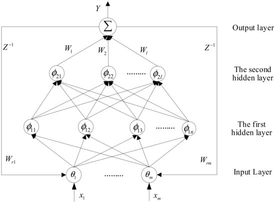
Figure 1.
Double hidden layer recurrent neural network.
The signal propagation and the results of each layer are explained as follows:
Layer 1—Input layer: The number of nodes in the input layer and the number of input signals are the same. Usually, the tracking error and the derivative of the error are selected as the input signal. Each input node is related to the output at the previous moment, and the corresponding feedback weight is defined as . Therefore, the i-th node output in the input layer is computed as:
where is the input of neural network, the feedback weight is , the output of the input layer is .
Layer 2—First hidden layer: The proposed network has two hidden layers. In this layer, the Gaussian activation function is used to initially extract the input feature information. Therefore, the Gaussian function output of j-th node is calculated as:
where the center vector and base width vector are defined as and . Finally, output vector of the first hidden layer is .
Layer 3—Second hidden layer: The purpose of the second hidden layer is to realize the nonlinear mapping from low latitude to high latitude. We also choose the Gaussian function as the activation function. In addition, there is no special requirement for the number of nodes in the first and second hidden layers. Finally, the second hidden layer output of the k-th node is designed as:
where is a center, base width is , output of the second hidden layer is .
Layer 4—Output layer: It is a linear map. Each node in the second hidden layer is linked to the output layer by a weight . The DHL-RNN output is expressed as:
where is the weights of output layer.
4. Controller Design and Stability Analysis
We first introduce a dynamic terminal sliding mode surface that not only ensures fast error convergence but also reduces chattering. Then the sliding mode control law is derived, and additionally, a FTDO is added to the control law to estimate the lumped unknown disturbance. Finally, the neural network proposed in section IV is introduced to approximate the switching gain in the sliding mode control law.
The purpose of the SMC law is to realize the compensation current tracking its reference current . In order to design the control law, we first define the tracking error and its derivative , then the error is .
Consider a terminal sliding mode surface:
where , is a positive constant to ensure Hurwitz stability, and .
Assumption 1.
Considering terminal function,,is a continuous differentiable function in,, when,is limited in interval. In order to obtain global robustness, set,,. When,,,.
According to Assumption 1, the following terminal function is constructed as:
Due to the inherent chattering problem of sliding mode, we construct a new switching function by differentiating the traditional switching function . Therefore, a dynamic terminal sliding mode surface is designed as:
where is a strictly positive constant.
Ignoring the lumped unknown disturbance , the first derivative of Equation (19) can be obtained:
Defining , we can get the ideal equivalent control term:
where .
After considering the lumped uncertainty , a FTDO is introduced to compensate for the disturbance:
A switching control item is designed to ensure the robustness as:
Finally, the designed dynamic terminal sliding mode control law based on disturbance compensation is derived:
where .
Remark 1.
Assumption 1 defines a terminal function, which requires the global stability of the sliding mode surface, and the tracking error of the system converges to zero within a finite time. The above requirements for dynamic terminal sliding surface are proved in [8]. For the control law (24), the switching gain has a decisive effect on the control performance. What we have to explain is that the choice of gain is not as large as possible. Excessive gain will bring obvious chattering. On the contrary, the system with too small gain is unstable. Therefore, we will use the DHLRNN to approximate the switching gain, so that the switching gain can reach the optimal value.
In order to find the adaptive law later, we will derive the approximation error in the neural network.
A DHLRNN is designed to approximate the switching control term, the following equation is true:
where is the minimum error between the ideal and actual values.
The optimal parameter is expressed as:
Considering that the optimal parameters cannot be obtained, we use the output of DHLRNN as the estimated value of the switching term. The following equation can be derived:
where is the estimated value of the optimal parameter .
Therefore, the approaching switching control term is:
Approximation error between actual and estimated value is obtained as:
where .
The Taylor series expansion of at , , , , is derived:
where is high-order term, is the derivative of to respectively. The above partial derivative is the Jacobian matrix determinant, like:
Taking the above derivative results (32)–(36) into the approximation error (29), we can obtain the following equation:
where is a lumped higher-order approximation error term, assumed to be bounded by .
Figure 2 is a block diagram of the proposed adaptive DTSMC using the FTDO. From the Figure 2, the designed controller consists of an equivalent control item, an approximate switching control item, and a compensated disturbance item.
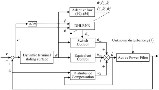
Figure 2.
Block diagram of the proposed FTDO-based DTSMC method.
The detailed information is developed as:
where .
Theorem 3.
Consider a dynamics (4) with the lumped unknown disturbances . If a FTDO is constructed as (5), and the control law is selected as Equation (38), then as long as the parameters of the control law and the observer are reasonably selected, the compensation current can track the reference current within a finite time, which means that the system is stable.
Proof.
According to the description of Remark 1, the observer error of the FTDO will eventually tend to be a finite constant, so we choose the following Lyapunov candidate function:
Considering the unknown disturbance of single-phase APF, deriving the dynamic terminal sliding mode surface (19) again yields:
Finding the first derivative of the Lyapunov candidate function (39) and bringing Equation (40) into it deduces:
where .
Equation (41) involves the control law before approximation, we add and subtract a control law after approximation, and we can get:
Bringing the approximation error (37) into (42) yields:
Finally, the following adaptive laws are selected:
Let , we can get:
Let , we can get:
Let , we can get:
Let , we can get:
Let , we can get:
Let , we can get:
where , , , , , is an adjustable constant.
After the adaptive laws (44)–(49) are selected, the first derivative of Lyapunov function is simplified as:
where is the upper bound of the higher-order approximation error of the neural network, and are the upper bounds of the observer error. In addition, we define a lumped observer error . From Equation (50), as long as we can guarantee that the switching gain approximated by the DHLRNN is greater than the upper bound of the lumped error, i.e., , then . Based on Lyapunov stability theory and Barbalat’s lemma, the control law (38) designed in this paper can ensure that the equilibrium point of the system is stable, which means . Once the conditions are met, by global stability, then the sliding mode surface is established, and finally by solving differential equations , the tracking error eventually tends to zero . □
5. Simulation Study
This part takes a single-phase parallel active power filter as the control object, and adopts the proposed strategy for the first-order dynamic model obtained by the averaging method to realize the current tracking control task. The circuit model diagram of APF is given in Figure 3. The effectiveness, reliability, and practical feasibility of the novel control strategy for APF system is verified on MATLAB/Simulink. The following introduces the simulation experiment where the comparative results are also carried out. In the simulation process, the CPU is i5-8300H (2.30 GHz), the system is 64-bit, and the version of MATLAB is 2019b. The control task is to design the controller to output an appropriate duty cycle to control the correct switching of the IGBT according to the calculated reference current, so as to realize the high-precision tracking control task of the current. Actually, three-phase active power filter has a symmetry structure based on single-phase parallel active power filter.
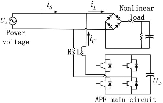
Figure 3.
Circuit model diagram of the APF system.
According to the derivation of the circuit model, the first-order dynamic model of APF can be obtained as
where , , , is the external disturbance. For the detailed modeling process, please refer to [18].
The parameters used in the system simulation are shown in Table 1. In this section, an adaptive DTSMC [7] is introduced as a comparison algorithm. The parameters in control law (adaptive DTSMC with FTDO) (36) are , the switching gain is approximated by a DHLRNN. The parameters of the FTDO are selected as , the structure of the DHLRNN is also selected as 2-4-3-1. The learning rate (31) is selected as , , , , , .

Table 1.
Model parameters of active power filter.
In the simulation process, the following three aspects are analyzed: (1) before APF compensation, (2) steady-state compensation process, (3) dynamic compensation process. In order to simulate the operating state of the grid system, the single-phase APF is linked to the grid system at , and a dynamic nonlinear load shown in Table 1 is connected to the grid system at , then the dynamic load that has been connected to the grid is separated at . It is worth noting that when we measure the THD value, the time mentioned later is the start measurement time, and the measurement period is selected as 5 periods.
Figure 4 is the grid current change curve under two control algorithms. From Figure 4a,b, when the APF is not linked to the grid, the power supply current is severely distorted. The THD value at is 38.61%. After , the single-phase APF starts to work, and the power current under the two algorithms was rapidly compensated to the sinusoidal waveform. Even if the non-linear load changes, the current curve is still sinusoidal waveform.
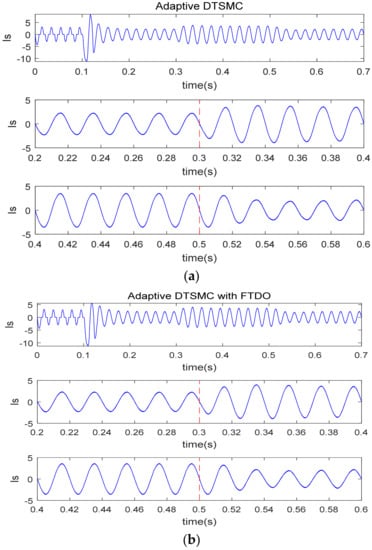
Figure 4.
Source current curve before and after compensation under two control algorithms (unit of y-axis of is A). (a) Adaptive DTSMC; (b) Adaptive DTSMC with FTDO.
Figure 5 is the harmonic current tracking curve under the two algorithms. No matter which algorithm is used, the harmonic compensation current can track the reference current in a short time. From Figure 5a, when the nonlinear load changes, the tracking effect of the adaptive DTSMC method suddenly becomes worse, while the proposed algorithm in this paper has better harmonic suppression property. In order to further compare the tracking effect, we have drawn the tracking error curve as shown in Figure 6. It is obvious that when the proposed algorithm is applied to the current controller, the tracking error is smoother, and the error range is smaller.
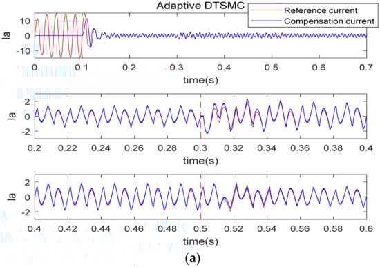
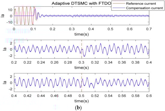
Figure 5.
Harmonic current tracking curve under two control algorithms (unit of y-axis of is A). (a) Adaptive DTSMC; (b) adaptive DTSMC with FTDO.
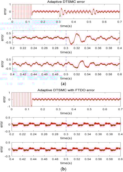
Figure 6.
Tracking error curve under two control algorithms. (a) Adaptive DTSMC; (b) adaptive DTSMC with FTDO.
The tracking curve of the voltage outer loop control is shown in Figure 7, and the gain of the PI controller is selected as . It is worth noting that although the controllers can be designed separately, in fact there is an indirect correlation between the current inner loop and the voltage outer loop. If the DC-side voltage cannot be stabilized, then the current inner loop control performance will be affected. From Figure 7, under the same PI control gain, the voltage outer loop tracking effect is very ideal, which means that the comparative simulation we conducted in the current loop is reasonable.
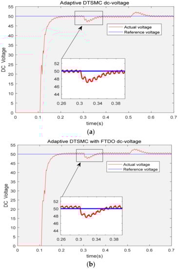
Figure 7.
DC side voltage tracking curve under two control algorithms (unit of y-axis is Volt). (a) Adaptive DTSMC; (b) adaptive DTSMC with FTDO.
Figure 8 is the control input curve under the two algorithms. Since the same sliding mode surface is adopted, the change trend of the control input is the same. In addition, the control input will be modulated into a switching signal by triangular wave, so we can ignore the amplitude of the control input.
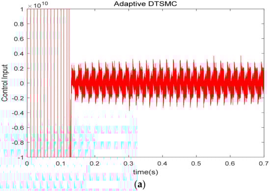
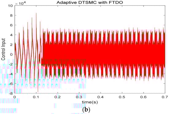
Figure 8.
Control input curve under two control algorithms (unit of y-axis of is A). (a) Adaptive DTSMC; (b) adaptive DTSMC with FTDO.
In order to directly reflect the steady-state and dynamic compensation performance under the two algorithms, Table 2 is the summary of the distortion rate change of the reflecting THD values measured at different time, showing the THD value of the proposed controller is reduced from 38.61% before compensation to 2.26% of the steady-state performance, and when an additional nonlinear load is increased, the THD is further reduced to 1.57%. When the nonlinear load is reduced again, the total harmonic distortion rate is 2.27%. Compared with the simple adaptive DTSMC law, the proposed method has better steady-state and dynamic-steady compensation effects.
Table 2.
Harmonic distortion rate of two algorithms at different times.
The proposed method applies a FTDO, and the disturbance compensation term (21) is added to the control law (24). However, it is worth discussing whether the disturbance term estimated by the observer is accurate, if not, it may affect the control accuracy of the system. Considering the output of the FTDO (6), the output estimates the state variable of the system , the output estimates the lumped unknown disturbance , and the output estimates the first derivative of the unknown disturbance .
It is not difficult to find that the integral of the observer output can be deduced, i.e., . Therefore, we can compare the observed value with the actual system state , if they are equal, it can indicate that the designed FTDO is effective. Finally, we can conclude that the observer’s estimate of the lumped unknown disturbance and its derivative are correct, and the disturbance compensation term is valid. Figure 9 is a comparison of the estimated value and actual harmonic compensation current . Regardless of the trend or amplitude, the curves of observed value and actual values are remarkably similar.
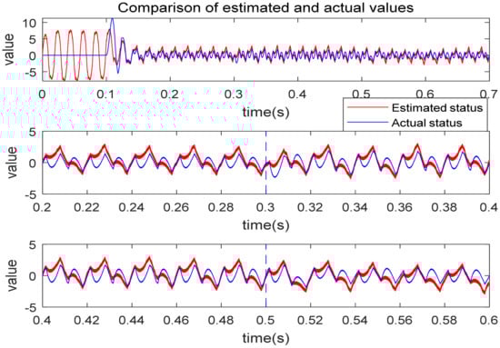
Figure 9.
Comparison of the estimated and actual values.
Figure 10 is the output of the disturbance compensation term. There is still a slight error between the observed value and the actual value in Figure 10, which will also cause a slight error in the estimated value of Figure 10. In fact, the smaller observation error can be ignored. In the stability proof (50), we have deduced that as long as the approximated switching gain is greater than the total integration error, i.e., , the stability of the system can be guaranteed. In other words, the observation error of the FTDO can be compensated by the switching gain.
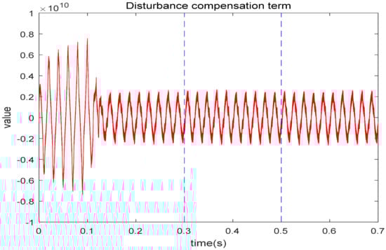
Figure 10.
Disturbance compensation term.
Since the DHLRNN is applied to approximate the switching gain, it can be seen from Figure 11 that the switching gain satisfies . The adaptive curves of the DHLRNN are shown in Figure 12, Figure 13, Figure 14, Figure 15, Figure 16 and Figure 17. It is shown that all parameters can converge to stable values because the role of the two hidden layers enables the network to have faster convergence speed and convergence accuracy under fewer nodes.
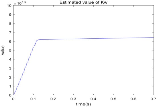
Figure 11.
The output of the DHLRNN.
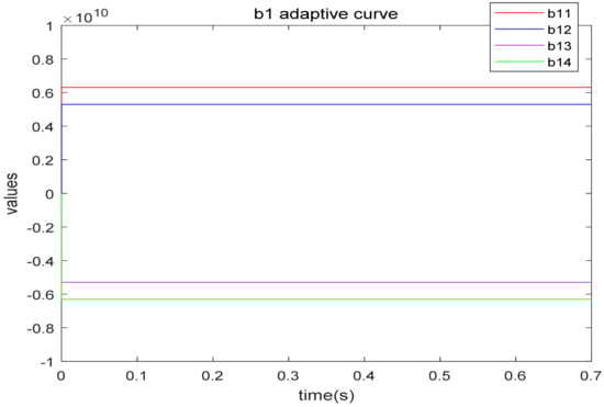
Figure 12.
Adaptive parameter B1 curve.
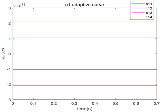
Figure 13.
Adaptive parameter C1 curve.
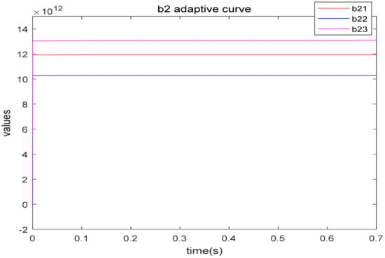
Figure 14.
Adaptive parameter B2 curve.
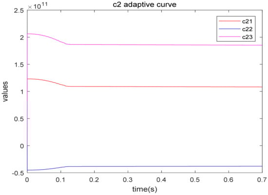
Figure 15.
Adaptive parameter C2 curve.
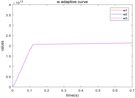
Figure 16.
Adaptive parameter W curve.
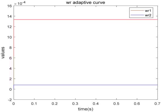
Figure 17.
Adaptive parameter Wr curve.
6. Conclusions
The current tracking control problem of nonlinear system has been investigated through an adaptive DTSMC technique with a FTDO in this paper. The merits of DSMC and TSMC are successfully combined to improve the convergence speed and reduce the chattering problems of traditional sliding mode controller. By combining the advantages of DMSC and TSMC, DTSM surface is designed, which can not only weaken chattering but also ensure the tracking error can finitely converge to zero. A FTDO is proposed to remove the negative impact of matched and mismatched disturbances on the control performance, where the disturbance compensation term is added to the DSMC law. A DHLRNN is presented to approximate the optimal switching gain, and all parameters in the neural network can converge to stable values because the role of the two hidden layers enables the network to have faster convergence speed and convergence accuracy under fewer nodes.
Finally, numerical simulation experiments show that the proposed method has effective compensation performance. Compared with the existing methods, the proposed algorithm has better dynamic compensation capabilities with the decreasing of 1% THD. Experimental validation by implementing the proposed method on the actual system in real-time is needed in the next research steps. Considering the superior control performance, the presented approach can be further extended to other power electronic controls.
Author Contributions
Conceptualization, J.F.; methodology, Y.F.; software, Y.C.; validation, Y.C.; writing—original draft preparation, Y.C.; writing—review and editing, Y.F.; project administration, J.F.; funding acquisition, J.F. All authors have read and agreed to the published version of the manuscript.
Funding
This work is partially supported by National Science Foundation of China under Grant No. 61873085.
Data Availability Statement
Not applicable.
Conflicts of Interest
The authors declare no conflict of interest.
References
- Yao, X.; Park, J.; Dong, H.; Guo, L.; Lin, X. Robust Adaptive Nonsingular Terminal Sliding Mode Control for Automatic Train Operation. IEEE Trans. Syst. Man Cybern. Syst. 2019, 49, 2406–2415. [Google Scholar] [CrossRef]
- Fei, J.; Wang, Z.; Pan, Q. Self-Constructing Fuzzy Neural Fractional-Order Sliding Mode Control for Active Power Filter. IEEE Trans. Neural Netw. Learn. Syst. 2022. Available online: https://ieeexplore.ieee.org/abstract/document/9768195 (accessed on 4 May 2022). [CrossRef]
- Young, K.; Utkin, V.; Ozguner, U. A control engineer's guide to sliding mode control. IEEE Trans. Control Syst. Technol. 1999, 7, 328–342. [Google Scholar] [CrossRef]
- Vu, M.T.; Le, T.-H.; Thanh, H.L.N.N.; Huynh, T.-T.; Van, M.; Hoang, Q.-D.; Do, T.D. Robust Position Control of an Over-actuated Underwater Vehicle under Model Uncertainties and Ocean Current Effects Using Dynamic Sliding Mode Surface and Optimal Allocation Control. Sensors 2021, 21, 747. [Google Scholar] [CrossRef] [PubMed]
- Lopac, N.; Bulic, N.; Vrkic, N. Sliding Mode Observer-Based Load Angle Estimation for Salient-Pole Wound Rotor Synchronous Generators. Energies 2019, 12, 1609. [Google Scholar] [CrossRef]
- Yang, Y.; Yan, Y. Backstepping sliding mode control for uncertain strict-feedback nonlinear systems using neural-network- based adaptive gain scheduling. J. Syst. Eng. Electron. 2018, 29, 580–586. [Google Scholar]
- Fei, J.; Chen, Y. Dynamic Terminal Sliding Mode Control for Single-Phase Active Power Filter Using Double Hidden Layer Recurrent Neural Network. IEEE Trans. Power Electron. 2020, 35, 9906–9924. [Google Scholar]
- Mozayan, S.; Saad, M.; Vahedi, H. Sliding Mode Control of PMSG Wind Turbine Based on Enhanced Exponential Reaching Law. IEEE Trans. Ind. Electron. 2016, 63, 6148–6159. [Google Scholar] [CrossRef]
- Wang, Y.; Feng, Y.; Zhang, X.; Liang, J. A New Reaching Law for Antidisturbance Sliding-Mode Control of PMSM Speed Regulation System. IEEE Trans. Power Electron. 2020, 35, 4117–4126. [Google Scholar] [CrossRef]
- Wang, Z.; Fei, J. Fractional-Order Terminal Sliding Mode Control Using Self-Evolving Recurrent Chebyshev Fuzzy Neural Network for MEMS Gyroscope. IEEE Trans. Fuzzy Syst. 2022, 30, 2747–2758. [Google Scholar] [CrossRef]
- Sami, I.; Ullah, S.; Ali, Z.; Ullah, N.; Ro, J. A Super Twisting Fractional Order Terminal Sliding Mode Control for DFIG-Based Wind Energy Conversion System. Energies 2020, 13, 2158. [Google Scholar] [CrossRef]
- Feng, Y.; Han, F.; Yu, X. Chattering free full-order sliding-mode control. Automatica 2014, 50, 1310–1314. [Google Scholar] [CrossRef]
- Liu, J.; Sun, F. A novel dynamic terminal sliding mode control of uncertain nonlinear systems. J. Control. Theory Appl. 2007, 5, 189–193. [Google Scholar] [CrossRef]
- Fei, J.; Chen, Y. Fuzzy Double Hidden Layer Recurrent Neural Terminal Sliding Mode Control of Single-Phase Active Power Filter. IEEE Trans. Fuzzy Syst. 2021, 29, 3067–3081. [Google Scholar] [CrossRef]
- Fei, J.; Wang, Z.; Liang, X. Adaptive Fractional Sliding Mode Control of Micro gyroscope System Using Double Loop Recurrent Fuzzy Neural Network Structure. IEEE Trans. Fuzzy Syst. 2022, 30, 1712–1721. [Google Scholar] [CrossRef]
- Xu, B.; Zhang, R. Composite Neural Learning Based Nonsingular Terminal Sliding Mode Control of MEMS Gyroscopes. IEEE Trans. Neural Netw. Learn. Syst. 2020, 31, 1375–1386. [Google Scholar] [CrossRef]
- Fei, J.; Wang, Z.; Fang, Y. Self-Evolving Chebyshev Fuzzy Neural Fractional-Order Sliding Mode Control for Active Power Filter. IEEE Trans. Ind. Inform. 2022. Available online: https://ieeexplore.ieee.org/abstract/document/9745783 (accessed on 31 March 2022). [CrossRef]
- Fei, J.; Liu, L. Real-Time Nonlinear Model Predictive Control of Active Power Filter Using Self-Feedback Recurrent Fuzzy Neural Network Estimator. IEEE Trans. Ind. Electron. 2022, 69, 8366–8376. [Google Scholar] [CrossRef]
- Levant, A. Higher-order sliding modes, differentiation and output-feedback control. Int. J. Control 2003, 76, 924–941. [Google Scholar] [CrossRef]
- Shtessel, Y.; Shkolnikov, I.A.; Levant, A. Smooth second-order sliding modes: Missile guidance application. Automatica 2007, 43, 1470–1476. [Google Scholar] [CrossRef]
- Wang, H.; Shi, L.; Man, Z.; Zheng, J.; Li, S.; Yu, M.; Jiang, C.; Kong, H.; Cao, Z. Continuous Fast Nonsingular Terminal Sliding Mode Control of Automotive Electronic Throttle Systems Using Finite-Time Exact Observer. IEEE Trans. Ind. Electron. 2018, 65, 7160–7172. [Google Scholar] [CrossRef]
- Wang, Z.; Li, S.; Li, Q. Continuous Nonsingular Terminal Sliding Mode Control of DC-DC Boost Converters Subject to Time-Varying Disturbances. IEEE Trans. Circuits Syst. II Express Briefs 2020, 67, 2552–2556. [Google Scholar] [CrossRef]
- Yang, J.; Li, S.; Su, J.; Yu, X. Continuous nonsingular terminal sliding mode control for systems with mismatched disturbances. Automatica 2013, 49, 2287–2291. [Google Scholar] [CrossRef]
- Yang, J.; Li, S.; Yu, X. Sliding-Mode Control for Systems With Mismatched Uncertainties via a Disturbance Observer. IEEE Trans. Ind. Electron. 2013, 60, 160–169. [Google Scholar] [CrossRef]
- Li, Y.; Liu, Y.; Tong, S. Observer-based neuro-adaptive optimized control for a class of strict-feedback nonlinear systems with state constraints. IEEE Trans. Neural Netw. Learn. Syst. 2021, 33, 3131–3145. [Google Scholar] [CrossRef]
- Li, Y.; Zhang, J.; Liu, W.; Tong, S. Observer-Based Adaptive Optimized Control for Stochastic Nonlinear Systems with Input and State Constraints. IEEE Trans. Neural Netw. Learn. Syst. 2021. Available online: https://ieeexplore.ieee.org/abstract/document/9463406 (accessed on 23 June 2021). [CrossRef]
- Shao, X.; Shi, Y. Neural Adaptive Control for MEMS Gyroscope With Full-State Constraints and Quantized Input. IEEE Trans. Ind. Inform. 2020, 16, 6444–6454. [Google Scholar] [CrossRef]
- Hou, S.; Fei, J. A Self-Organizing Global Sliding Mode Control and Its Application to Active Power Filter. IEEE Trans. Power Electron. 2020, 35, 7640–7652. [Google Scholar] [CrossRef]
- Hua, M.; Zheng, D.; Deng, F. H∞ filtering for nonhomogeneous Markovian jump repeated scalar nonlinear systems with multiplicative noises and partially mode-dependent characterization. IEEE Trans. Syst. Man Cybern. Syst. 2021, 51, 3180–3192. [Google Scholar] [CrossRef]
- Chu, Y.; Fei, J.; Hou, S. Adaptive Global Sliding Mode Control for Dynamic Systems Using Double Hidden Layer Recurrent Neural Network Structure. IEEE Trans. Neural Netw. Learn. Syst. 2019, 31, 1297–1309. [Google Scholar] [CrossRef]
Publisher’s Note: MDPI stays neutral with regard to jurisdictional claims in published maps and institutional affiliations. |
© 2022 by the authors. Licensee MDPI, Basel, Switzerland. This article is an open access article distributed under the terms and conditions of the Creative Commons Attribution (CC BY) license (https://creativecommons.org/licenses/by/4.0/).