Abstract
Peakons and periodic peakons are two kinds of special symmetric traveling wave solutions, which have important applications in physics, optical fiber communication, and other fields. In this paper, we study the orbital stability of peakons and periodic peakons for a generalized Camassa–Holm equation with quadratic and cubic nonlinearities (mCH–Novikov–CH equation). It is a generalization of some classical equations, such as the Camassa–Holm (CH) equation, the modified Camassa–Holm (mCH) equation, and the Novikov equation. By constructing an inequality related to the maximum and minimum of solutions with the conservation laws, we prove that the peakons and periodic peakons are orbitally stable under small perturbations in the energy space.
MSC:
35B35; 37K05; 37K45
1. Introduction
This paper is concerned with the following generalized Camassa–Holm equation with quadratic and cubic nonlinearities (mCH–Novikov–CH equation) [1]
where , , or , , are all real-valued parameters. Qin, Yan, and Guo [1] introduced Equation (1), and showed Equation (1) possesses symmetric peakons and periodic peakons. Equation (1) is a generalization of some classical equations, such as the Camassa–Holm (CH) equation, the modified Camassa–Holm (mCH) equation, and the Novikov equation.
When , and , Equation (1) reduces to the CH Equation [2]
which was derived as a model for the unidirectional propagation of the shallow water waves over a flat bottom [3,4]. Using the method of recursive operators, Fokas and Fuchssteiner [5] found that Equation (2) has the bi-Hamiltonian structure with an infinite number of conserved quantities. Equation (2) has many important properties: existence of peaked solitons [2,6], complete integrability [2,5], and wave breaking phenomena [7,8,9]. It is remarkable that Equation (2) possesses the peakon in the form of
which was proved orbitally stable by Constantin and Strauss in [10]. Inspired by [10], Lenells [11] studied the stability of periodic peakons for Equation (2). Then, by means of variational methods, Constantin and Molinet proved the orbital stability of the peakon [12]. The orbital stability of multi-peakon solutions for Equation (2) was discussed in [13]. It is remarkable that Wang, Han, and Lu [14] showed that the b-family of the Novikov equation possessed some symmetric traveling wave solutions. In addition, Ray and Sahoo [15] constructed the analytical exact solutions of Riesz Time-Fractional Camassa–Holm Equation via modified homotopy analysis method (MHAM).
The following Degasperis–Procesi (DP) equation that is similar to Equation (2)
is also completely integrable. Lin and Liu [16] proved the orbital stability of the single peakons for the DP equation.
When , , and , Equation (1) becomes the Novikov equation
which is an integrable Camassa–Holm type equation with cubic nonlinearity. Liu, Liu, and Qu [17] studied the orbital stability of the peaked solitons for Equation (5). In addition, Wang and Tian [18] extended Lenell’s approach to discuss the orbital stability of periodic peakons for Equation (5). Moreover, Moon [19] proved the existence of peaked traveling wave solutions for the generalized -Novikov equation with nonlocal cubic and quadratic nonlinearities.
When , , and , Equation (1) is transformed into the integral mCH equation with cubic nonlinearities
which was obtained by the tri-Hamiltonian duality approach [20]. In [21], the peakons and periodic peakons of Equation (6) were proved orbitally stable in the energy space. Liu, Liu, and Olver [22] proved that the peakons and periodic peakons for a generalization of the modified Camassa–Holm equation were obitally stable. In [23], Moon studied the dynamical stability of periodic peaked solitary waves for the generalized modified Camassa–Holm equation. Chen, Di, and Liu [24] showed the stability of peaked waves for the mCH–Novikov equation without restrictions on the sign of the momentum density. On the base of [24], Chen, Deng, and Qiao [25] first verify that the existence of global peakon and periodic peakon solutions and the orbital stability of peakons and periodic peakons for a nonlinear quartic Camassa–Holm equation.
It is not difficult to find that the special case of Equation (1) in this paper just corresponds to the above-mentioned special equations. In other words, it can be seen that studying the stability of the peakon of Equation (1) will further deepen the understanding of the stability of peakons of the CH-type equation if , , are non-zero. By [1], we know that Equation (1) has the following form of single peaked traveling wave solutions
where
Equation (1) also has the following form of periodic peaked traveling wave solutions in [1]
where means the floor function or the greatest integer function and
Here, we denote .
When , there is the above-mentioned Figure 1. In addition, when , represents the maximum value corresponding to the periodic peakon, and, similarly, represents the minimum value of the periodic peakon. The definition of Equations (7) and (9) will be described exhaustively in Section 2. Moreover, Equation (1) has multi-peaked traveling wave solutions in [1]. In [26], Hwang and Moon proved the existence of periodic peaked solitary waves to the equation of -Camassa–Holm–Novikov. Then, the exact solutions can be attained by eliminating logarithmic nonlinearity [27], symmetry analysis [28], and the modifed Khater method [29]
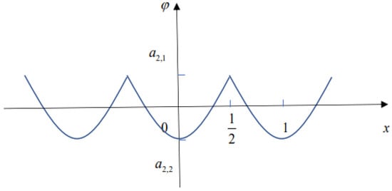
Figure 1.
The profile of periodic peakon for .
Notice that the peaked function (3) is the traveling wave solutions to Equation (2) and travels with speed c and has a corner (that is, a finite jump in its derivative) at its peak of height c. Furthermore, the peaked function (3) is a soliton: two traveling waves reconstitute their shape and size after interacting with each other [30]. As for the periodic peakon, through [31], we know that periodic plane waves, termed swell, do not change along the wave crest, and move the same in any direction parallel to the crest line. Similarly, the interaction between periodic traveling waves does not change their shapes. Importantly, Equation (2) is the first such equation found that models the solitons’ interaction of peaked traveling waves. Thus, we consider quantitative analysis of the stability of peakons and periodic peakons for Equation (1) in this paper.
The peakon can generate another solitary wave with different speed and phase translation under small perturbations. The stability mentioned in this paper refers to the orbital stability, that is, the wave with initial profile always maintains a similar distance from the peakon for all later time, and has the similar shape of wave all the time. Inspired by the work of [10,11], in this paper, we will prove that the symmetric peakons and periodic peakons of Equation (1) are orbitally stable under small perturbations in the energy space.
In order to facilitate the readers to understand the following Theorem 1, we briefly explain the several professional terms. Firstly, it is found that the -norm of the solitary wave u is equivalent to the conserved quantity . In other words, energy space refers to space. Secondly, the definition of strong solutions is not described in detail in Section 1; see Section 2 for details.
Theorem 1.
Let or , where and are referred to the real field and the unit circle. For every , there is a such that, if is a solution to Equation (1) with
then
where and is an extreme point where the function attains its maximum. Therefore, the peakons (or periodic peakons) are orbitally stable.
From Figure 2, we can intuitively see that the wave u with the initial profile is always close enough to the peakon in later times. The translation does not change the properties of the wave u, as long as u and satisfy the condition (11), they will reach orbital stability in the subsequent time.
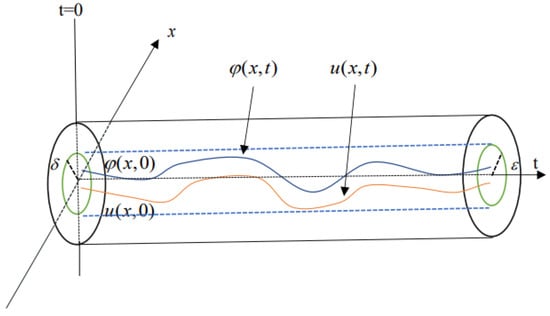
Figure 2.
The graphical example of orbital stability.
The outline of this paper is as follows: In Section 2, we briefly recall the well-posedness result, three conservation laws, and the important definition for Equation (1). In Section 3, the orbital stability for peakons and periodic peakons are established in the energy space -norm. In Section 4, we give a brief conclusion.
2. Preliminary
In this section, the well-posedness result, two important definitions, and three conservation laws of Equation (1) are shown below.
Definition 1
Proposition 1
([1]). Let with . Then, there exists a time such that the initial value problem of Equation (1) has a unique strong solution , and the map is continuous from a neighborhood of in into .
Definition 2
([1]). Given the initial data , the function is said to be a weak solution to the Cauchy problem (1) if it satisfies the following identity:
for any smooth test function . If u is a weak solution on for every , then it is called a global weak solution. Note that u can be formulated by the Green function p in [1] as
where * denotes the convolution product on , defined by
Notice that Equation (1) has the conservation laws as follows:
Those conservation laws will be helpful for our proof of the orbital stability. Furthermore, the conservation laws of time fractional coupled equations can be obtained in [32,33,34]. In addition, we can easily verify that is the conservation law of the Equation (1) by integration by parts in Appendix A.
3. Stability
3.1. Stability of Peakons
In this subsection, we firstly prove the orbital stability of peakons for when . In addition, the profile of peakon for has been shown in Figure 3. For the sake of simplicity, we consider proving the orbital stability of the following form of peakon:
where . Similarly, when , the orbital stability of peakons can be proved in the same way. Without loss of generality, we assume that and c are positive constants.
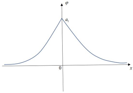
Figure 3.
The profile of peakon for .
Replacing u by , we find that
Then, we consider the expansion of the conservation law around the peakon in the -norm.
Lemma 1.
For any and ,
Proof.
It follows from integration by parts that
Thus, we have
which completes the proof of Lemma 1. □
Lemma 1 sets up a global identity about conserved quantities. We will determine the disturbance term of maximum height of u and through the following lemmas, so as to quantitatively estimate the global disturbance between the maximum value of the solitary wave u by disturbance near the peakon and the peakon .
Lemma 2.
For , , let , then
Proof.
Assume that attains the maximum at , then , and define
It is easy to show that
On the other hand, we define by
Then, we have
By the Young’s inequality,
Therefore, we have finished the proof of Lemma 2. □
Lemma 3.
For all , , if with , then
and
where
Proof.
We observe that
The equality holds if and only if v is proportional to a translate of . Note that
Similarly,
Now, we first estimate and .
By means of Hölder’s inequality, one finds
where .
According to Young’s inequality, we have
Due to the following Gagliardo–Nirenberg–Sobolev inequality,
where is an undermined constant. Using Equation (35), we obtain
where C is independent of . Due to , we thus obtain
where the constant depends only the norm . Then, from the above three estimations, one deduces
Thus, we complete the proof of Lemma 3. □
Lemma 4.
For all , , let . If
and
for some , then
3.2. Stability of Periodic Peakons
In this subsection, we will prove the stability of periodic peakon of Equation (1). In particular, we have shown the profile of periodic peakon by Figure 1. When , it is obvious that the periodic peaked function for ,
which can be extended to the whole line. Here, we still use with the interval and treat all functions on as periodic functions with the period T on the entire line. For the convenience of calculation, we set .
Equation (1) has the following three conservation laws:
where the functionals defined in Equation (45) are independent of .
For an integer , let be the Sobolev space of all square integrable functions with distributional derivatives for . These Hilbert spaces are endowed with the following inner product:
A function is said to be a solution to Equation (1) on with the period if the equation holds in the distribution sense. Clearly, is continuous on with a peak at . Therefore, we calculate that
Thus, by integration by parts, we obtain
and
Lemma 5.
For all and ,
Proof.
We calculate
Due to , we obtain
Thus, we complete the proof of Lemma 5. □
Similar to Lemma 1, Lemma 5 also constructs the global identity related to the conserved quantity, and combined with the following several lemmas, the proof of the orbital stability of periodic peakons can be completed.
Lemma 6.
For any positive , let
be the function defined by
Then, we have
where and .
Proof.
Noted that the periodic peakon satisfies the following equation:
Let be a positive function and write and . Let and satisfy , . Similarly, we need to define the real function as follows:
and extend it periodically to the real line. Then,
Next, we define
A direct calculation leads to
and
Since
and
we have
It follows from Young’s inequality that
Combining with Equation (67), we see that
which completes the proof of Lemma 6. □
Similar to Lemma 2.5 in [11], we obtain the following properties of .
Lemma 7.
The peaked function φ satisfies the following relations:
Lemma 8.
Suppose , then
Here, “equal” holds if and only if for some , that is, f is a peakon.
Proof.
For , we have
Since
we obtain
where “equal” holds true if and only if f and are proportional. Taking the maximum of Equation (73) over completes the proof of Lemma 8. □
Lemma 9.
If , then and are continuous functions of .
Proof.
By Lemma 8, for , we have
which implies that is continuous. The continuity of is evident since , which finish the proof of Lemma 9. □
Suppose , . Then, we obtain
Following the work from Lemma 2.9 in [11], we obtain the following lemma:
Lemma 10.
Let be a solution of Equation (1). Given a small neighborhood of in , there is a such that
Finally, we prove Theorem 1 for the case of .
Proof.
Let be a solution of Equation (1) and assume that we are given an . Then, we choose a neighborhood of small enough that if . We can find a in Lemma 10 such that Equation (76) holds. Then, choosing a smaller if necessary, we may suppose
Therefore, we use Lemma 7 to deduce that
where is any point satisfying .
Therefore, we have proved Theorem 1 for the case of . □
4. Conclusions
In this paper, we obtain the orbital stability of symmetric peakons and periodic peakons for the mCH–Novikov–CH equation. The mCH–Novikov–CH equation is a generalization of some classical equations, such as the Camassa–Holm (CH) equation, the modified Camassa–Holm (mCH) equation, and the Novikov equation. The proof is inspired by [10,11]. In particular, we construct a polynomial inequality related to the maximum and the minimum with the conservation laws, which plays an important role in our proof of the orbital stability of peakons and periodic peakons for Equation (1). From the perspective of energy space , Theorem 1 shows that the shape of the (periodic) wave generated near the (periodic) peakon remains unchanged under the slight perturbation.
Author Contributions
Investigation, K.Z., J.Y. and S.T.; writing—review and editing, K.Z., J.Y. and S.T.; funding acquisition, K.Z., J.Y. and S.T. All authors contributed equally in the preparation of this paper. All authors have read and agreed to the published version of the manuscript.
Funding
This work have partially been supported by the Guangxi Key Laboratory of Cryptography and Information Security (No. GCIS202134) and the Innovation Project of Guangxi Graduate Education (No. YCSW2022291).
Institutional Review Board Statement
Not applicable.
Informed Consent Statement
Not applicable.
Data Availability Statement
Not applicable.
Conflicts of Interest
The authors declare no conflict of interest.
Appendix A
In Appendix A, the proof of conserved quantities are as follows. In order to prove the qualities , is independent of t, we set . Thus, we have
By using integration by parts, one finds
From the above calculations, we can see that
that is, is independent of t and is the conservation law of Equation (1).
References
- Qin, G.; Yan, Z.; Guo, B. The cauchy problem and multi-peakons for the mCH–Novikov–CH equation with quadratic and cubic nonlinearities. J. Dyn. Differ. Equ. 2022, 2022, 1–60. [Google Scholar] [CrossRef]
- Camassa, R.; Holm, D. An integrable shallow water equation with peaked solitons. Phys. Rev. Lett. 1993, 71, 1661–1664. [Google Scholar] [CrossRef]
- Constantin, A.; Lannes, D. The hydrodynamical relevance of the Camassa–Holm and Degasperis-Procesi equations. Arch. Ration. Mech. Anal. 2009, 192, 165–186. [Google Scholar] [CrossRef]
- Camassa, R.; Holm, D.; Hyman, J. A new integrable shallow water equation. Adv. Appl. Mech. 1994, 31, 1–33. [Google Scholar]
- Fuchssteiner, B.; Fokas, A. Symplectic structures, their Bäcklund transformations and hereditary symmetries. Physics D 1982, 4, 47–66. [Google Scholar] [CrossRef]
- Alber, M.; Camassa, R.; Holm, D. The geometry of peaked solitons and billiard solutions of a class of integrable PDE’s. Lett. Math. Phys. 1994, 32, 137–151. [Google Scholar] [CrossRef]
- Constantin, A.; Escher, J. Wave breaking for nonlinear nonlocal shallow water equations. Acta Math. 1998, 181, 229–243. [Google Scholar] [CrossRef]
- Constantin, A.; Escher, J. Global existence and blow-up for a shallow water equation. Ann. Sci. Norm. Super. 1998, 26, 303–328. [Google Scholar]
- Li, Y.; Olver, P. Well-posedness and blow-up solutions for an integrable nonlinearly dispersive model wave equation. J. Differ. Equ. 2000, 162, 27–63. [Google Scholar] [CrossRef]
- Constantin, A.; Strauss, W. Stability of peakons. Commun. Pure Appl. Math. 2000, 53, 603–610. [Google Scholar] [CrossRef]
- Lenells, J. Stability of periodic peakons. Int. Math. Res. Not. 2004, 10, 485–499. [Google Scholar] [CrossRef]
- Constantin, A.; Molinet, L. Orbital stability of solitary waves for a shallow water equation. Physics D 2001, 157, 75–89. [Google Scholar] [CrossRef]
- Dika, K.; Molinet, L. Stability of multipeakons. Ann. I. H. Poincaré-An. 2009, 26, 1517–1532. [Google Scholar] [CrossRef]
- Wang, T.; Han, X.; Lu, Y. On the solutions of the b-family of Novikov equation. Symmetry 2021, 13, 1765. [Google Scholar] [CrossRef]
- Ray, S.S.; Sahoo, S. Traveling wave solutions to Riesz time-fractional Camassa–Holm equation in modeling for shallow-water waves. J. Comput. 2015, 10, 061026. [Google Scholar]
- Lin, Z.; Liu, Y. Stability of peakons for the Degasperis-Procesi equation. Commun. Pure. Appl. Math. 2009, 62, 125–146. [Google Scholar] [CrossRef]
- Liu, X.; Liu, Y.; Qu, C. Stability of peakons for the Novikov equation. J. Math. Pure Appl. 2014, 101, 172–187. [Google Scholar] [CrossRef]
- Wang, Y.; Tian, L. Stability of periodic peakons for the Novikov equation. arXiv 2018, arXiv:1811.05835v1. [Google Scholar]
- Moon, B. Single peaked traveling wave solutions to a generalized μ-Novikov equation. Adv. Nonlinear Anal. 2021, 10, 66–75. [Google Scholar] [CrossRef]
- Olver, P.; Rosenau, P. Tri-hamiltonian duality between solitons and solitary-wave solutions having compact support. Phys. Rev. E 1996, 53, 1900–1906. [Google Scholar] [CrossRef]
- Qu, C.; Liu, X.; Liu, Y. Stability of peakons for an integrable modified Camassa–Holm equation with cubic nonlinearity. Commun. Math. Phys. 2013, 322, 967–997. [Google Scholar] [CrossRef]
- Liu, X.; Liu, Y.; Olver, P.J.; Qu, C. Orbital stability of peakons for a generalization of the modified Camassa–Holm equation. Nonlinearity 2014, 27, 2297–2319. [Google Scholar] [CrossRef]
- Moon, B. Orbital stability of periodic peakons for the generalized modified Camassa–Holm equation. Discrete. Contin. Dyn. Syst. Ser. A 2021, 14, 4409–4437. [Google Scholar] [CrossRef]
- Chen, R.; Di, H.; Liu, Y. Stability of peaked solitary waves for a class of cubic quasilinear shallow-water equations. Int. Math. Res. Not. 2022, 2022, rnac032. [Google Scholar] [CrossRef]
- Chen, A.; Deng, T.; Qiao, Z. Stability of peakons and periodic peakons for a nonlinear quartic Camassa–Holm equation. Mon. Hefte. Math. 2022, 198, 251–288. [Google Scholar] [CrossRef]
- Hwang, G.; Moon, B. Periodic peakons to a generalized μ-Camassa–Holm-Novikov equation. Appl. Anal. 2021, 2021, 1–11. [Google Scholar] [CrossRef]
- Izgi, Z.P.; Saglam, F.N.; Sahoo, S. A partial offloading algorithm based on intelligent sensing. Int. J. Mod. Phys. B 2022, 36, 2500977. [Google Scholar] [CrossRef]
- Sahoo, S.; Saha, R.S. New soliton solutions of fractional Jaulent-Miodek system with symmetry analysis. Symmetry 2020, 12, 1001. [Google Scholar] [CrossRef]
- Tripathy, A.; Sahoo, S. New optical behaviours of the time-fractional Radhakrishnan-Kundu-Lakshmanan model with Kerr law nonlinearity arise in optical fibers. Opt. Quantum Electron. 2022, 54, 232. [Google Scholar] [CrossRef]
- Drazin, P.G.; Johnson, R.S. Solitons: An Introduction; Cambridge University Press: Cambridge, UK, 1989. [Google Scholar]
- Constantin, A.; Escher, J. Analyticity of periodic traveling free surface water waves with vorticity. Ann. Math. 2011, 173, 559–568. [Google Scholar] [CrossRef]
- Sahoo, S.; Saha, R.S. Invariant analysis with conservation law of time fractional coupled Ablowitz–Kaup–Newell–Segur equations in water waves. Waves Random Complex Media 2020, 30, 530–543. [Google Scholar] [CrossRef]
- Sahoo, S.; Saha, R.S. On the conservation laws and invariant analysis for time-fractional coupled Fitzhugh-Nagumo equations using the Lie symmetry analysis. Eur. Phys. J. Plus 2019, 134, 83. [Google Scholar] [CrossRef]
- Sahoo, S.; Saha, R.S. Lie symmetries analysis and conservation laws for the fractional Calogero–Degasperis–Ibragimov–Shabat equation. Int. J. Geom. Methods Mod. Phys. 2018, 15, 1–11. [Google Scholar] [CrossRef]
Publisher’s Note: MDPI stays neutral with regard to jurisdictional claims in published maps and institutional affiliations. |
© 2022 by the authors. Licensee MDPI, Basel, Switzerland. This article is an open access article distributed under the terms and conditions of the Creative Commons Attribution (CC BY) license (https://creativecommons.org/licenses/by/4.0/).