
Discrete Dynamic Model of a Disease-Causing Organism Caused by 2D-Quantum Tsallis Entropy


Abstract
:1. Introduction
2. Methodology
2.1. Quantum Calculus
2.2. Quantum Entropy
2.3. 2D-Quantum Discrete System
3. Stability of DCO
3.1. 2D-Quantum Reproductive Ratio
- The survival function, also known as the reliability function, is one of the methods used to formulate and display survival statistics. It provides the likelihood that a patient, plan, or other object of concern would survive longer than any given time. It gives the likelihood that a subject will live for more time than χ.
- A function like the exponential distribution may be able to accurately represent the survival times distribution. There are many distributions frequently used in survival analysis. These distributions are presented by parameters [36].
- Entropy is changed from a measure of information to a statistical tool by the entropy optimization principle, which also incorporates the 2D-QTE. It is safe to use this knowledge to define CFR because the greater maximum entropy belongs to fractional Tsallis entropy [37].
3.2. 2D-Fractal Dimensions
4. Conclusions
Author Contributions
Funding
Institutional Review Board Statement
Informed Consent Statement
Data Availability Statement
Conflicts of Interest
References
- Jackson, F.H., XI. On q-functions and a certain difference operator. Earth Environ. Sci. Trans. R. Soc. Edinb. 1909, 46, 253–281. [Google Scholar] [CrossRef]
- Ibrahim, R.W.; Ajaj, A.M.; Al-Saidi, N.M.G.; Balean, D. Similarity Analytic Solutions of a 3D-Fractal Nanofluid Uncoupled System Optimized by a Fractal Symmetric Tangent Function. Comput. Model. Eng. Sci. 2022, 130, 221–232. [Google Scholar] [CrossRef]
- Al-Azawi; Al-Saidi, R.J.N.M.G.; Jalab, H.A.; Kahtan, H.; Ibrahim, R.W. Efficient classification of covid-19 CT scans by using q-transform model for feature extraction. PeerJ Comput. Sci. 2021, 7, e553. [Google Scholar] [CrossRef]
- Ibrahim, Y.; Yahya, R.W.H.; Mohammed, A.J.; Al-Saidi, N.M.G.; Baleanu, D. Mathematical Design Enhancing Medical Images Formulated by a Fractal Flame Operator. Intell. Autom. Soft Comput. 2022, 32, 937–950. [Google Scholar] [CrossRef]
- Farhan, K.A.; Al-Saidi, N.M.G.; Maolood, A.T.; Nazarimehr, F.; Hussain, I. Entropy analysis and image encryption application based on a new chaotic system crossing a cylinder. Entropy 2019, 21, 958. [Google Scholar] [CrossRef]
- Nicolas, B. A Short History of Mathematical Population Dynamics; Springer: London, UK, 2011. [Google Scholar]
- Kermack, W.O.; McKendrick, A.G. A contribution to the mathematical theory of epidemics. Proc. R. Soc. A 1927, 115, 700–721. [Google Scholar]
- Chang, Z.; Meng, X.; Zhang, T. A new way of investigating the asymptotic behaviour of a stochastic sis system with multiplicative noise. Appl. Math. Lett. 2019, 87, 80–86. [Google Scholar] [CrossRef]
- Huang, W.; Han, M.; Liu, K. Dynamics of an SIS reaction-diffusion epidemic model for disease transmission. Math. Biosci. Eng. 2017, 7, 51–66. [Google Scholar]
- Liu, M.; Chang, Y.; Wang, H.; Li, B. Dynamics of the impact of twitter with time delay on the spread of infectious diseases. Int. J. Biomath. 2018, 11, 1850067. [Google Scholar] [CrossRef]
- Newman, M.E.J. The structure and function of complex networks. SIAM Rev. 2003, 45, 167–256. [Google Scholar] [CrossRef]
- Momani, S.; Ibrahim, R.W.; Hadid, S.B. Susceptible-infected-susceptible epidemic discrete dynamic system based on Tsallis entropy. Entropy 2020, 22, 769. [Google Scholar] [CrossRef] [PubMed]
- Pastor-Satorras, R.; Vespignani, A. Epidemics and immunization in scale-free networks. In Handbook of Graphs and Networks; Wiley: Berlin, Germany, 2003. [Google Scholar]
- Colizza, V.; Pastor-Satorras, R.; Vespignani, A. Reaction–diffusion processes and metapopulation models in heterogeneous networks. Nat. Phys. 2007, 3, 276–282. [Google Scholar] [CrossRef]
- Kang, H.; Sun, M.; Yu, Y.; Fu, X.; Bao, B. Spreading dynamics of an SEIR model with delay on scale-free networks. IEEE Trans. Netw. Sci. Eng. 2018, 7, 489–496. [Google Scholar] [CrossRef]
- Kuśmierz, Ł.; Toyoizumi, T. Infection curves on small-world networks are linear only in the vicinity of the critical point. Proc. Natl. Acad. Sci. USA 2021, 118, e2024297118. [Google Scholar] [CrossRef] [PubMed]
- Bae, H.J.; Lee, S. Investigation of SIS epidemics on dynamic network models with temporary link deactivation control schemes. Math. Biosci. Eng. 2022, 19, 6317–6330. [Google Scholar] [CrossRef]
- Boole, G. A Treatise on the Calculus of Difference Equations; Cambridge University Press: Cambridge, UK, 1860; Volume 2, p. 17. [Google Scholar]
- Wolfgang, H. Über Orthogonalpolynome, die q-Differenzengleichungen genügen. Math. Nachrichten 1949, 2, 4–34. [Google Scholar]
- Chakrabarti, R.; Jagannathan, R. A (p, q)-oscillator realization of two-parameter quantum algebras. J. Phys. Math. Gen. 1991, 24, L711. [Google Scholar] [CrossRef]
- Tsallis, C. Possible generalization of Boltzmann-Gibbs statistics. J. Stat. Phys. 1988, 52, 479–487. [Google Scholar] [CrossRef]
- Ramírez-Reyes, A.; Hernández-Montoya, A.R.; Herrera-Corral, G.; Domínguez-Jiménez, I. Determining the entropic index q of Tsallis entropy in images through redundancy. Entropy 2016, 18, 299. [Google Scholar] [CrossRef]
- Machado, J.T. Fractional order generalized information. Entropy 2014, 16, 2350–2361. [Google Scholar] [CrossRef]
- Machado, J.T. Fractional Renyi entropy. Eur. Phys. J. Plus 2019, 134, 1–10. [Google Scholar] [CrossRef]
- Ibrahim, R.W.; Moghaddasi, Z.; Jalab, H.A.; Noor, R.M. Fractional differential texture descriptors based on the Machado entropy for image splicing detection. Entropy 2015, 17, 4775–4785. [Google Scholar] [CrossRef]
- Hasan, A.M.; Al-Jawad, M.M.; Jalab, H.A.; Shaiba, H.; Ibrahim, R.W.; AL-Shamasneh, A.A.R. Classification of Covid-19 Coronavirus, Pneumonia and Healthy Lungs in CT Scans Using Q-Deformed Entropy and Deep Learning Features. Entropy 2020, 22, 517. [Google Scholar] [CrossRef] [PubMed]
- Ibrahim, R.W. The fractional differential polynomial neural network for approximation of functions. Entropy 2013, 15, 4188–4198. [Google Scholar] [CrossRef]
- Ibrahim, R.W. Utility function for intelligent access web selection using the normalized fuzzy fractional entropy. Soft Comput. 2020, 1–8. [Google Scholar] [CrossRef]
- Jalab, H.A.; Subramaniam, T.; Ibrahim, R.W.; Kahtan, H.; Noor, N.F.M. New Texture Descriptor Based on Modified Fractional Entropy for Digital Image Splicing Forgery Detection. Entropy 2019, 21, 371. [Google Scholar] [CrossRef]
- Ibrahim, W.R.; Darus, M. Analytic study of complex fractional Tsallis’ entropy with applications in CNNs. Entropy 2018, 20, 722. [Google Scholar] [CrossRef] [PubMed]
- Allen, L.J.S.; Van den Driessche, P. The basic reproduction number in some discrete-time epidemic models. J. Differ. Equ. Appl. 2008, 14, 1127–1147. [Google Scholar] [CrossRef]
- Yong, T. Maximum entropy method for estimating the reproduction number: An investigation for COVID-19 in China. Phys. Rev. E 2020, 102, 03216. [Google Scholar]
- Tsallis, C.; Tirnakli, U. Predicting COVID-19 peaks around the world. Front. Phys. 2020, 8, 217. [Google Scholar] [CrossRef]
- Pennings, P. COVID19 in numbers- R0, the case fatality rate and why we need to flatten the curve.webm Date: 11 March 2020.
- Heffernan, J.M.; Smith, R.J.; Wahl, L.M. Perspectives on the basic reproduction ratio. J. R. Soc. Interface 2005, 2, 281–293. [Google Scholar] [CrossRef] [PubMed]
- Dayi, H.; Huang, Q.; Gao, J. A new entropy optimization model for graduation of data in survival analysis. Entropy 2012, 14, 1306–1316. [Google Scholar]
- Vijay, P.S.; Sivakumar, B.; Cui, H. Tsallis entropy theory for modeling in water engineering: A review. Entropy 2017, 19, 641. [Google Scholar]
- Talu, S. Multifractal geometry in analysis and processing of digital retinal photographs for early diagnosis of human diabetic macular edema. Curr. Eye Res. 2013, 38, 781–792. [Google Scholar] [CrossRef] [PubMed]
- Ott, E. Chaos in Dynamical Systems; Cambridge University Press: Cambridge, UK; New York, NY, USA, 1993; ISBN 978-0-521-43799-8. [Google Scholar]
- Sam, Y.; Lakshminarayanan, V. Fractal Dimension and Retinal Pathology: A Meta-Analysis. Appl. Sci. 2021, 11, 2376. [Google Scholar]
- Huang, F.; Dashtbozorg, B.; Zhang, J.; Bekkers, E.; Abbasi-Sureshjani, S.; Berendschot, T.T.J.M.; Ter Haar Romeny, B.M. Reliability of using retinal vascular fractal dimension as a biomarker in the diabetic retinopathy detection. J. Ophthalmol. 2016, 2016, 6259047. [Google Scholar] [CrossRef]
- Renyi, A. On the dimension and entropy of probability distributions. Acta Math. Acad. Sci. Hung. 1959, 10, 193–215. [Google Scholar] [CrossRef]
- Alberti, T.; Donner, R.V.; Vannitsem, S. Multiscale fractal dimension analysis of a reduced order model of coupled ocean-atmosphere dynamics. Earth Syst. Dyn. Discuss. 2021, 12, 1–24. [Google Scholar] [CrossRef]

| Figure | ||
|---|---|---|
| 2 | 0.4 | 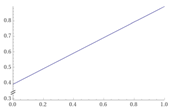 |
| 3 | 0.21 | 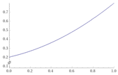 |
| 4 | 0.12 | 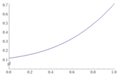 |
Publisher’s Note: MDPI stays neutral with regard to jurisdictional claims in published maps and institutional affiliations. |
© 2022 by the authors. Licensee MDPI, Basel, Switzerland. This article is an open access article distributed under the terms and conditions of the Creative Commons Attribution (CC BY) license (https://creativecommons.org/licenses/by/4.0/).
Share and Cite
Al-Saidi, N.M.G.; Yahya, H.; Obaiys, S.J. Discrete Dynamic Model of a Disease-Causing Organism Caused by 2D-Quantum Tsallis Entropy. Symmetry 2022, 14, 1677. https://doi.org/10.3390/sym14081677
Al-Saidi NMG, Yahya H, Obaiys SJ. Discrete Dynamic Model of a Disease-Causing Organism Caused by 2D-Quantum Tsallis Entropy. Symmetry. 2022; 14(8):1677. https://doi.org/10.3390/sym14081677
Chicago/Turabian StyleAl-Saidi, Nadia M. G., Husam Yahya, and Suzan J. Obaiys. 2022. "Discrete Dynamic Model of a Disease-Causing Organism Caused by 2D-Quantum Tsallis Entropy" Symmetry 14, no. 8: 1677. https://doi.org/10.3390/sym14081677
APA StyleAl-Saidi, N. M. G., Yahya, H., & Obaiys, S. J. (2022). Discrete Dynamic Model of a Disease-Causing Organism Caused by 2D-Quantum Tsallis Entropy. Symmetry, 14(8), 1677. https://doi.org/10.3390/sym14081677