1. Introduction
Recently, many authors [
1,
2,
3,
4] have introduced and constructed generating functions for new families of special polynomials including two parametric kinds of polynomials, such as Bernoulli, Euler, and Genocchi. They have given the fundamental properties of these polynomials, and they have also established more identities and relations among trigonometric functions with two parametric kinds of special polynomials by using generating functions. Special polynomials have important roles in several subjects, such as mathematics, approximation theory, engineering, and theoretical physics. By applying the partial derivative operator to these generating functions, some derivative formulas and finite combinatorial sums involving the aforementioned polynomials and numbers are obtained. In addition, these special polynomials allow the derivation of different useful identities in a fairly straightforward way and help introduce new families of special polynomials. The array-type polynomials can be seen in combinatorial mathematics and play a crucial role in the principle and applications of arithmetic. Hence, a wide variety of idea and combinatorics experts have extensively studied their residences and received a series of exciting results (see [
5,
6,
7,
8,
9]). By inspiring and motivating the above polynomials, in this study, we propose defining a parametric type of
-array-type polynomials by introducing the two specific
q-exponential generating functions. In addition, we show many formulations and family members for those polynomials, such as a few implicit summation formulas, differentiation policies, and correlations with the earlier polynomials with the aid of utilizing a collection manipulation approach.
The concern with
q-calculus started in the 19th century due to its packages in various fields such as mathematics, physics, and engineering. The definitions and notations of
q-calculus reviewed here are taken from [
10,
11].
The
q-analogue of the shifted factorial
is given by
The
q-analogue of a complex number
and of the factorial function is given by
The Gauss
q-binomial coefficient
is given by
The
q-analogue of the function
is given by
The
q-analogues of exponential functions are given by
These two functions are related by the following equation (see [
10,
11,
12]):
Remark 1. It is not difficult to see that [
10]
Definition 1. Let x and y be two complex numbers and ω be a nonnegative integer. We define the q-addition in the following way (see [
13]
): The
q-derivative operator is defined by
where
provided that
f is differentiable at
.
The
q-derivative fulfills the following product and quotient rules:
Definition 2. The q-trigonometric functions areandwhere , . Lemma 1. Let and . Then, we have
(2)where , . Lemma 2. Let and . Then, we have
The Apostol-type
q-Bernoulli polynomials
of the order
, the Apostol-type
q-Euler polynomials
of the order
, and the Apostol-type
q-Genocchi polynomials
of the order
are defined as follows, respectively (see [
14,
15]):
Kang and Ryoo [
13] introduced the
q-Bernoulli and
q-Euler polynomials, defined by the following respective equations:
and
Kang and Ryoo proved the following (see [
13,
16]):
and
where
and
For
, the generalized
-Stirling numbers of the second kind
are given by the following (see [
17,
18]):
Given that
, Equation (
19) reduces to the Stirling numbers of the second kind as follows:
The
-array-type polynomials
are defined by the following (see [
6]):
2. -Array-Type Polynomials of Complex Variables
In this section, we consider the
q-Cosine and
q-Sine
-array-type polynomials of complex variables and deduce some identities of these polynomials. First, we present the following definition:
On the other hand, we suppose that
Thus, by Equations (21) and (22), we have
and
From Equations (23) and (24), we find
and
Definition 3. Let . We define two parametric kinds of q-Cosine λ-array-type polynomials and q-Sine λ-array-type polynomials , which for a nonnegative integer n are defined, respectively, byand Note that .
From Equations (25)–(28), we have
Remark 2. For in Equations (27) and (28), we obtain a new type of q-Cosine λ-array-type polynomial and q-Sine λ-array-type polynomial , respectively, asand Remark 3. Letting in Definition 3, we find two parametric types of λ-array-type polynomials as follows (see [
6]
):and Now, we start with some basic properties of these polynomials.
Theorem 1. If we let , thenand Proof. By Equations (31) and (32), we can derive the following equations:
and
Therefore, by Equations (35) and (36), we find Equations (33) and (34). □
Theorem 2. If we let , thenand Proof. By using Equations (23) and (24), we obtained Equations (37) and (38), so we omitted the proof. □
Theorem 3. If we let , thenand Proof. Now, we have
which proves Equation (
39). The proof of Equation (
40) is similar. □
Theorem 4. If we let , thenand Proof. By changing
x with
in Equation (
27), we have
which completes the proof for Equation (
41). The result for Equation (
42) can be proven in a similar manner. □
Theorem 5. If we let , thenand Proof. Equation (
27) yields
which proves Equation (
43). Equations (44)–(46) can be similarly derived. □
Theorem 6. If we let , then the following formula holds true:and Proof. By using Definition 3, we can easily prove Equations (47) and (48). Therefore, we omitted the proof. □
Theorem 7. The following relation holds true:and Proof. By using Definition 3, we can easily obtain
Comparing the coefficients of
on both sides of the last equality leads to the desired identity in Equation (
49). The relation in Equation (
50) follows easily in a similar way. □
Theorem 8. The following summation formulas are true:and Proof. Consider the following equality:
By making use of Equation (7) for
, through Equations (7) and (27), we find that
Now, if we compare the coefficients of
on both sides of Equation (
53), we reach the formula in Equation (
51). The relation in Equation (
52) can be derived in a similar manner. □
Theorem 9. Let and r be any real numbers. Then, we have
Proof. By substituting
into
in the generating function of
q-Cosine array-type polynomials, we have
Through a similar method, we can find the following equation:
By adding Equations (56) with (57), we can derive result (1) of Theorem 9.
For results (2) in Theorem 9, we also can find the following equations:
Using Equation (
59) appropriately, we can find result (2) in Theorem 9. □
Corollary 1. If we let , thenand Corollary 2. For in Corollary 1, we haveand 3. Symmetric Structures of the Approximate Roots for q-Cosine λ-Array-Type Polynomials and Their Application
In this section, certain zeros of the q-Cosine -array-type polynomials and beautiful graphical representations are shown. Let .
A few of examples of these include
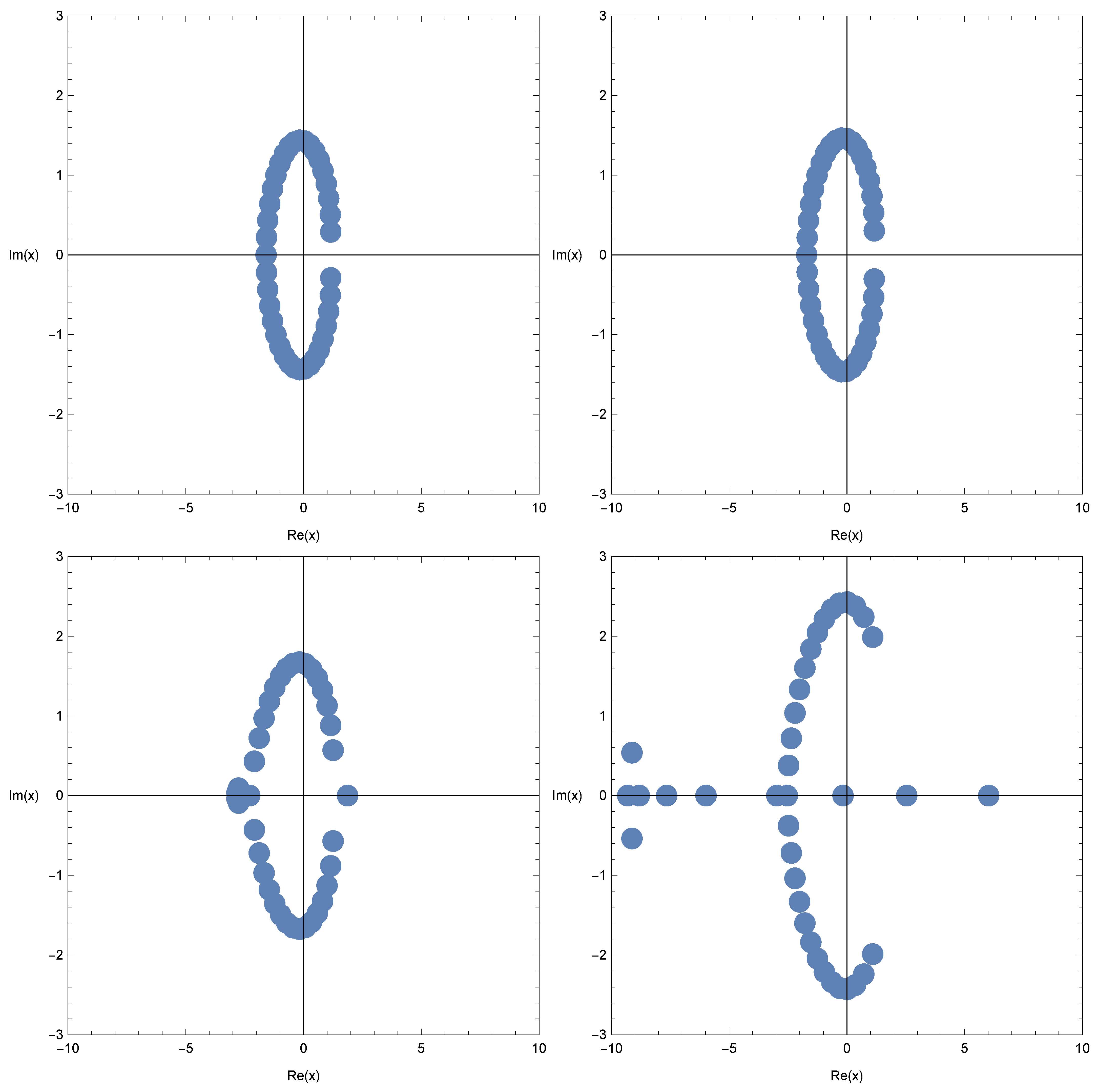
We investigated the beautiful zeros of the
q-Cosine
-array-type polynomials
by using a computer. We plotted the zeros of the
q-Cosine
-array-type polynomials
for
(
Figure 1).
In
Figure 1 (top left), we chose
and
. In
Figure 1 (top right), we chose
and
. In
Figure 1 (bottom left), we chose
and
. In
Figure 1 (bottom right), we chose
and
.
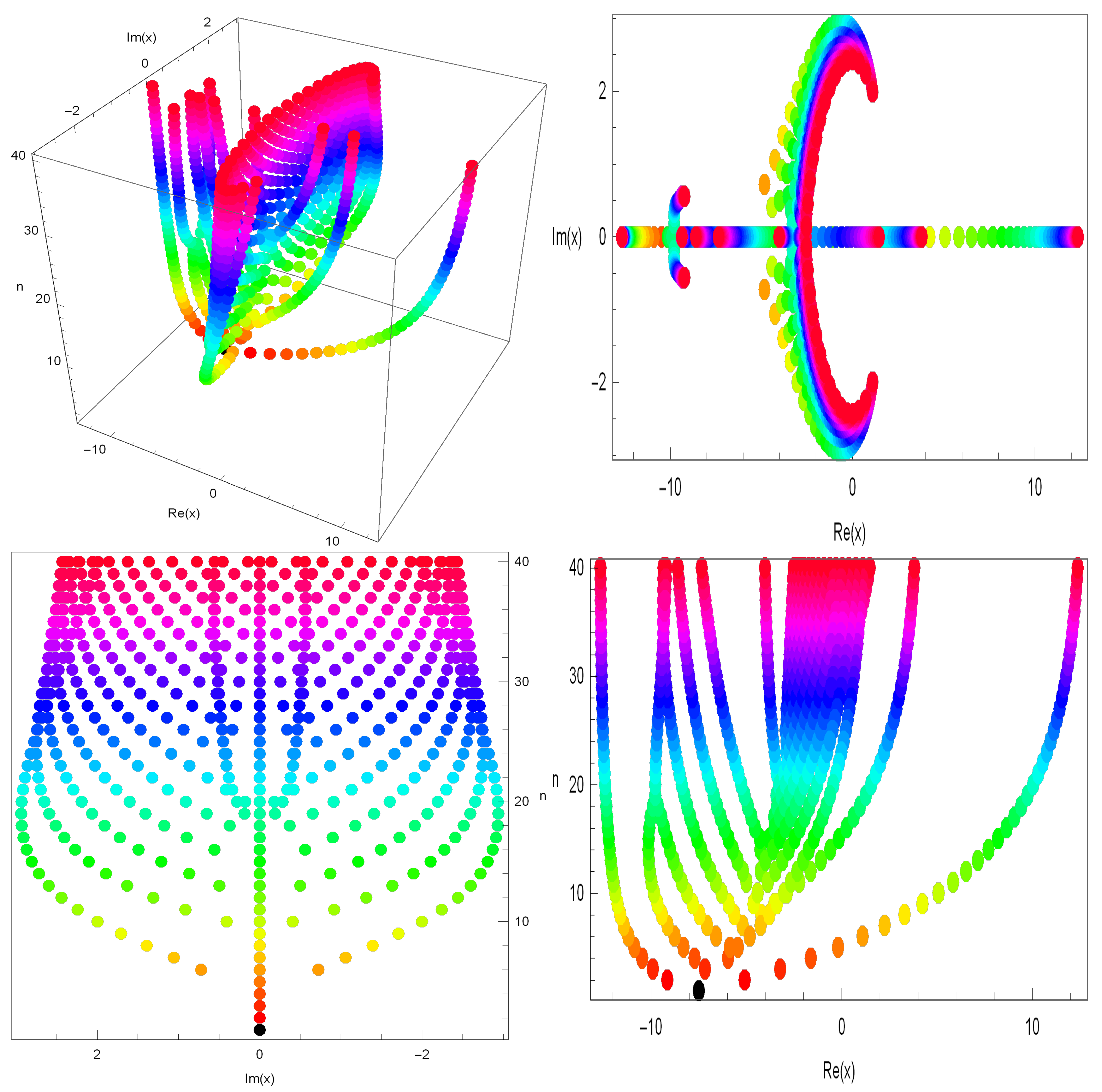
The stacks of zeros of the
q-Cosine
-array-type polynomials
for
, forming a 3D structure, are presented in
Figure 2.
In
Figure 2 (top left), we plotted the stacks of zeros of the
q-Cosine
-array-type polynomials
for
,
, and
In
Figure 2 (top right), we drew the
x and
y axes but no
z axis of the three dimensions. In
Figure 2 (bottom left), we drew the
y and
z axes but no
x axis of the three dimensions. In
Figure 2 (bottom right), we drew the
x and
z axes but no
y axis of the three dimensions.
We plotted the real zeros of the
q-Cosine
-array-type polynomials
for
(
Figure 3).
In
Figure 3 (top left), we chose
and
. In
Figure 3 (top right), we chose
and
. In
Figure 3 (bottom left), we chose
and
. In
Figure 3 (bottom right), we chose
and
.
Next, we calculated an approximate solution satisfying the
q-Cosine
-array-type polynomials
for
. The results are given in
Table 1.
4. Symmetric Structures of the Approximate Roots for q-Sine λ-Array-Type Polynomials and Their Application
In this section, certain zeros of q-Sine--array-type polynomials and beautiful graphical representations are shown. Let .
A few of these include the following:
We investigated the beautiful zeros of the
q-Sine
-array-type polynomials
by using a computer. We plotted the zeros of the
q-Cosine
-array-type polynomials
for
(
Figure 4).
In
Figure 4 (top left), we chose
and
. In
Figure 4 (top right), we chose
and
. In
Figure 4 (bottom left), we chose
and
. In
Figure 4 (bottom right), we chose
and
.
The stacks of zeros of the
q-Sine
-array-type polynomials
for
, forming a 3D structure, are presented in
Figure 5.
In
Figure 5 (top left), we chose
and
. In
Figure 5 (top right), we chose
and
. In
Figure 5 (bottom left), we chose
and
. In
Figure 5 (bottom right), we chose
and
.
Next, we calculated an approximate solution satisfying the
q-Sine
-array-type polynomials
for
. The results are given in
Table 2.
5. Conclusions
In this paper, using the q-Cosine polynomials and q-Sine polynomials, we introduced novel types of q-extensions of -array-type polynomials, and the features obtained multifarious homes and identities by using some collection manipulation techniques. Furthermore, we computed the q-quintessential representations and q-derivative operator policies for those polynomials. Moreover, we determined the approximate root movements of the brand new mentioned polynomials in a complicated plane, utilizing the Newton technique and illustrating them in figures. The shape of the approximate roots will pop out in diverse ways, depending on the circumstances of the variables, and there is a desire for new methods and theorems associated with this subject matter to be created and proven. We would like to continue to observe this line of study in the future.
Author Contributions
Conceptualization, W.A.K., C.S.R.; Formal analysis, M.S.A.; Funding acquisition, M.S.A.; Investigation, W.A.K.; Methodology, W.A.K., C.S.R. and M.S.A.; Project administration, C.S.R.; Software, W.A.K. and C.S.R.; Writing—original draft, W.A.K.; Writing—review & editing, W.A.K. and M.S.A. All authors have read and agreed to the published version of the manuscript.
Funding
This research received no external funding.
Institutional Review Board Statement
Not applicable.
Informed Consent Statement
Not applicable.
Data Availability Statement
No data were used to support this study.
Conflicts of Interest
The authors declare that they have no competing interests.
References
- Alam, N.; Khan, W.A.; Ryoo, C.S. A note on Bell-based Apostol-type Frobenius-Euler polynomials of complex variable with its certain applications. Mathematics 2022, 10, 2109. [Google Scholar] [CrossRef]
- Muhiuddin, G.; Khan, W.A.; Duran, U.; Al-Kadi, D. Some identities of the multi poly-Bernoulli polynomials of complex variable. J. Funct. Spaces 2021, 2021, 7172054. [Google Scholar] [CrossRef]
- Muhiuddin, G.; Khan, W.A.; Al-Kadi, D. Construction on the degenerate poly-Frobenius-Euler polynomials of complex variable. J. Funct. Spaces 2021, 2021, 3115424. [Google Scholar] [CrossRef]
- Nisar, K.S.; Khan, W.A. Notes on q-Hermite based unified Apostol type polynomials. J. Interdiscip. Math. 2019, 22, 1185–1203. [Google Scholar] [CrossRef]
- Acikgöz, M.; Araci, S.; Cangül, I.N. A note on the modified q-Bernstein polynomials for functions of several variables and their reflections on q-volkenborn integration. Appl. Math. Comput. 2011, 2018, 707–712. [Google Scholar]
- Cakić, N.P.; Milovanović, G.V. On generalized Stirling number and polynomials. Math. Balk. 2004, 18, 241–248. [Google Scholar]
- Khan, W.A. A note on q-analogue of degenerate Catalan numbers associated with p-adic Integral on . Symmetry 2022, 14, 1119. [Google Scholar] [CrossRef]
- Özger, F.; Aljimi, E.; Ersoy, M.T. Rate of weighted statistical convergence for generalized blending-type Bernstein-Kantorovich operators. Mathematics 2022, 10, 2027. [Google Scholar] [CrossRef]
- Khan, W.A. A note on q-analogues of degenerate Catalan-Daehee numbers and polynomials. J. Math. 2022, 2022, 9486880. [Google Scholar] [CrossRef]
- Jackson, H.F. q-Difference equations. Am. J. Math. 1910, 32, 305–314. [Google Scholar] [CrossRef]
- Jackson, H.F. On q-functions and a certain difference operator. Trans. R. Soc. Edinb. 2013, 46, 253–281. [Google Scholar] [CrossRef]
- Kang, J.Y.; Khan, W.A. A new class of q-Hermite based Apostol type Frobenius Genocchi polynomials. Commun. Korean Math. Soc. 2020, 35, 759–771. [Google Scholar]
- Kang, J.Y.; Ryoo, C.S. Various structures of the roots and explicit properties of q-cosine Bernoulli polynomials and q-sine Bernoulli polynomials. Mathematics 2020, 8, 463. [Google Scholar] [CrossRef]
- Mahmudov, N.I. q-analogues of the Bernoulli and Genocchi polynomials and the Srivastava-Pinter addition theorems. Discret. Dyn. Nat. Soc. 2012, 2012, 169348. [Google Scholar] [CrossRef]
- Mahmudov, N.I. On a class of q-Bernoulli and q-Euler polynomials. Adv. Diff. Equ. 2013, 2013, 108. [Google Scholar] [CrossRef]
- Ryoo, C.S.; Kang, J.Y. Explicit properties of q-Cosine and q-Sine Euler polynomials containing symmetric structures. Symmetry 2020, 12, 1247. [Google Scholar] [CrossRef]
- Jamei, M.J.; Milovanović, G.V.; Daǧli, M.C. A generalization of the array type polynomials. Math. Moravica 2022, 26, 37–46. [Google Scholar] [CrossRef]
- Luo, Q.M.; Srivastava, H.M. Some generalization of the Apostol-Genocchi polynomials and Stirling numbers of the second kind. Appl. Math. Comput. 2011, 217, 5702–5728. [Google Scholar] [CrossRef]
| Publisher’s Note: MDPI stays neutral with regard to jurisdictional claims in published maps and institutional affiliations. |
© 2022 by the authors. Licensee MDPI, Basel, Switzerland. This article is an open access article distributed under the terms and conditions of the Creative Commons Attribution (CC BY) license (https://creativecommons.org/licenses/by/4.0/).


