Double Penalized Expectile Regression for Linear Mixed Effects Model

Abstract

This paper constructs the double penalized expectile regression for linear mixed effects model, which can estimate coefficient and choose variable for random and fixed effects simultaneously. The method based on the linear mixed effects model by cojoining double penalized expectile regression. For this model, this paper proposes the iterative Lasso expectile regression algorithm to solve the parameter for this mode, and the Schwarz Information Criterion (SIC) and Generalized Approximate Cross-Validation Criterion (GACV) are used to choose the penalty parameters. Additionally, it establishes the asymptotic normality of the expectile regression coefficient estimators that are suggested. Though simulation studies, we examine the effects of coefficient estimation and the variable selection at varying expectile levels under various conditions, including different signal-to-noise ratios, random effects, and the sparsity of the model. In this work, founding that the proposed method is robust to various error distributions at every expectile levels, and is superior to the double penalized quantile regression method in the robustness of excluding inactive variables. The suggested method may still accurately exclude inactive variables and select important variables with a high probability for high-dimensional data. The usefulness of doubly penalized expectile regression in applications is illustrated through a case study using CD4 cell real data.

1. Introduction

Linear mixed effect model (LME) is an important statistical model, which is widely used in various fields. The LME model includes the fixed effect and random effect. The fixed effect is used to represent the general characteristics of the sample population, and the random effect is used to depict the divergences between individuals and the correlation between multiple observations. The structure and property of this model reveal substantial differences compared to the general linear models and complete random coefficient linear models. Compared with other linear models, the inclusion of random effects in the mixed effects model captures the correlation between the observed variables.

Maximum likelihood and least square method are the classical methods of estimation used for the LME model. However, the least square method leads to biased estimates when the data with heavy-tailed distribution or significant heteroscedasticity. Koenker and Bassett (1978) [1] considered the quantile regression to solve such problems by regressing covariates according to the conditional quantiles of response, and capture the regression models under the all quantiles. However, the sparsity of sample variable is an issue which can not be ignored when it involves the correction analysis of variables, that is not all variables have predictive roles on regression analysis. In practical applications, massive candidate variables can be used for modeling analysis and prediction. Retaining the incorrelated variables in the model for prediction is undesirable, where the retention of irrelevant variables will produce the large deviation and non-interpretability of the model. How to select variables effectively is a challenging topic for the linear mixed effects models. Similar to the general linear regression, replacing the different types of penalty terms in the quantile regression can achieve synchrosqueezing for coefficients to reach target of variable selection. For example, Tibshirani (1996) [2] proposed a Lasso method with penalty terms, and selected variables by squeeze parameters sparsely in quantile regression. Quantile Lasso regression constraints some coefficients of irrelevant variables to 0 when the sum of absolute values of coefficients is less than a pre-specified constant, which not only can acquire a more simplified model and select variables simultaneously, also solve the problem of data with sparsity. Next, Zou (2006) [3] gave the proof of the oracle properties of adaptive Lasso in generalized linear models. Biswas and Das (2021) [4] proposed a Bayesian approach of estimating the quantiles of multivariate longitudinal data. Koenker (2004) [5] proposed the $L_1$ penalty quantile regression based on random effects, which can estimates parameter through weighting random effects information of multiple quantiles. Wang (2018) [6] proposed a new semiparametric approach that uses copula to account for intra-subject dependence and approximates the marginal distributions of longitudinal measurements, given covariates, through regression of quantiles. Wu and Liu (2009) [7] proposed the SCAD and adaptive Lasso penalized quantile regression method, and gave the oracle properties in the situation of variable number unchanged. For different types of data, Peng (2021) [8] illustrated the practical utility of quantile regression in actual survival data analysis through two cases. Li (2020) [9] constructed a double penalized quantile regression method, and used the Lasso algorithm to solve the parameters. It proved that the estimated accuracy of the double penalized quantile regression is better than the other quantile regression. And according to the article above, we find that double penalized quantile regression model lacks accuracy and stability in excluding inactive variables. And expectile regression can accurately reflect the tail characteristics of the distribution, the variables of the model can be accurately selected. Therefore, in order to excluding inactive variables more accurately, this paper cojoin the double penalty terms into the expectile regression to obtain the double penalized expectile regression model.

Newey and Powell (1987) [10] replaced the $L_1$-norm loss function to $L_2$-norm loss function for weighted least-squares, and proposed expectile regression. It regresses the covariates based on the conditional expectile of the response to obtain the regression model under all expectiles level. Almanjahie et al. (2022) [11] investigated the nonparametric estimation of the expectile regression model for strongly mixed function time series data. Gu (2016) [12] proposed the regularized expectile regression to analysis heteroscedastictiy of high-dimensional data. Farooq and Steinwart (2017) [13] analysed a support vector machine type approach for estimating conditional expectiles. Expectile and quantile are metric indicators that capture the tail behavior of data distribution. When covariates make different impacts on the distributions of different response, such as right or left skew, the two metrics can not only decrease the effects of outliers on statistical inference, but also provide a more comprehensive characteristics of entire distribution. Therefore, quantile and expectile regression provide a more comprehensive relation between the covariates and response.

Quantile regression is the generalization of median regression, and expectile regression is the generalization of mean regression, so expectile regression inherits the computational convenience and sensitivity to the observation values. Especially in the financial field, researchers need the sensity of expectile regression to data. For panel data, the model proposed by Schulze and Kauermann (2017) [14] allows multiple covariates, and a semi-parametric approach with penalized splines is pursued to fit smooth expectile curves. For cross-sectional data, expectile regression models and its applications have been studied. Sobotha et al. (2013) [15] discussed the expectile confidence interval based on large sample properties; Zhao and Zhao (2018) [16] proposed the penalized expectile regression model with SCAD penalty with the proof of asymptotic property; Liao et al. (2019) [17] proposed penalized expectile regression with adaptive Lasso and SCAD penalty for variable selection, and gave the proof of oracle properties under independent but different distributions of error terms. Waldmannetal et al. (2017) [18] proposed a combined Bayesian method with weighted least squares to estimate complex expectile regression. Next, the newly proposed iterative Lasso-expectile regression algorithm is used to solve the estimation of parameters and variables selections. Xu and Ding (2021) [19] combined the elastic network punishment with expectile regression and constructed the elastic network penalized expectile regression model. For the underlying optimization problem, Farooq and Steinwart (2017) [20] proposed an efficient sequential-minimal-optimization-based solver and derived its convergence. For the model selection problem, Spiegel et al. (2017) [21] introduced several approaches on selection criteria and shrinkage methods to perform model selection in semiparametric expectile regression. Expectile regression has also received attention in the economic and financial sector, particularly in actuarial and financial risk management. Daouia et al. (2020) [22] derive joint weighted Gaussian approximations of the tail empirical expectile and quantile processes under the challenging model of heavy-tailed distributions. Ziegel (2013) [23] applied expectile regression to the field of risk measurement.

Expectile regression is widely used in various fields. Including economic field [11,14,17,22,23], biomedical field [12,19] and health field [15,18,21] etc. Therefore, the study of expectile regression has many practical significances, and it is very necessary to study it.

To select the important variables into the model and the inactive variables excluded from the model more accurately, this paper combines the linear mixed effect model with the expectile regression model, and cojoin penalty terms into the estimation of random and fixed effects to construct the double penalized expectile regression for linear mixed effects model. And the iterative Lasso-Expectile regression algorithm is used to solve parameters. The asymptotic property of double penalized expectile regression estimation is proved. The simulation studies will analysis the results of coefficient estimation and variable selection of the method proposed in this paper under different conditions, and the robustness of this method in excluding inactive variables is mainly studied. Finally, based on the research on the real data of CD4 cells, the practical utility difference between the double penalized quantile regression and the double penalized expectile regression are compared.

The rest of this paper is organized as follows. We propose the double penalized expectile regression method and the iterative Lasso expectile regression algorithm in Section 2. The convergence of the algorithm and the asymptotic properties of the model are given in Section 3. In Section 4, we present the simulation studies. And a real data example is illustrated in Section 5. Moreover, this method is compared with the existing double penalized quantile regression method in parameter estimation and variable selection in simulation studies and real data analysis. In Section 6, we give the conclusions. In Appendices, we show the proofs of lemmas and asymptotic properties, and some graphs and tables obtained by simulation studies.

2. Methodologies

In order to get the specific formula of the linear mixed effect double penalized expectile regression model, we introduce the LME model and summarize the estimation methods. And give the specific steps of iterative lasso-expectile regression algorithm. Then we discuss the selection criteria of penalty parameters.

2.1. Model and Estimation

Firstly, we consider the LME model

$$y_{ij}={\mathit{x}}_{ij}^{\mathrm{T}}\mathit{\beta }+{\mathit{z}}_{ij}^{\mathrm{T}}{\mathit{\alpha }}_i+r_{ij}, i=1,2,\cdots ,n,j=1,2,\cdots ,n_i,{\displaystyle \sum _i{n}_i}=N,$$

(1)

where $\mathit{\beta }(t)={\{{\beta }_1(t),\cdots ,{\beta }_h(t)\}}^T$ is the $h\times 1$ vector of fixed effects regression coefficients, ${\mathit{\alpha }}_i={({\alpha }_{i1},{\alpha }_{i2},\cdots ,{\alpha }_{il})}^{\mathrm{T}}$ is a $l\times 1$ vector of random effects. ${\mathit{x}}_{ij}^{\mathrm{T}}$ is the row vector of the known design matrix, ${\mathit{z}}_{ij}$ is the $l\times 1$ covariate associated with random effects, and $y_{ij}$ is the $j\mathrm{th}$ scalar of the ith subject’s continuous random variable. And we let ${\mathit{\alpha }}_i\sim N(\mathbf{0},\mathit{P})$, $r_i\sim N(\mathbf{0},{\mathit{Q}}_i)$. The Equation (1) can be expressed as

$${\mathit{y}}_i={\mathit{X}}_i\mathit{\beta }+{\mathit{Z}}_i{\mathit{\alpha }}_i+{\mathit{r}}_i, {\mathit{\alpha }}_i\sim N(\mathbf{0},\mathit{P}), {\mathit{r}}_i\sim N(\mathbf{0},{\mathit{Q}}_i), i=1,2,\dots ,n$$

(2)

where ${\mathit{X}}_i={({\mathit{x}}_{i1},{\mathit{x}}_{i2},\cdots ,{\mathit{x}}_{i{n}_i})}^{\mathrm{T}}$, ${\mathit{Z}}_i={({\mathit{z}}_{i1},{\mathit{z}}_{i2},\cdots ,{\mathit{z}}_{i{n}_i})}^{\mathrm{T}}$, ${\mathit{y}}_i={(y_{i1},y_{i2}\cdots ,y_{i{n}_i})}^{\mathrm{T}}$, and ${\mathit{r}}_i={({\mathit{r}}_{i1},{\mathit{r}}_{i2},\cdots ,{\mathit{r}}_{i{n}_i})}^{\mathrm{T}}$.

Next, we let $\mathit{Z}=\mathrm{diag}({\mathit{Z}}_1,{\mathit{Z}}_2,\cdots ,{\mathit{Z}}_n)$, $\mathit{r}=({\mathit{r}}_1^{\mathrm{T}},{\mathit{r}}_2^{\mathrm{T}},\cdots ,{\mathit{r}}_n^{\mathrm{T}}{)}^{\mathrm{T}}$, $\mathit{X}={({\mathit{X}}_1^{\mathrm{T}},{\mathit{X}}_2^{\mathrm{T}},\cdots ,{\mathit{X}}_n^{\mathrm{T}})}^{\mathrm{T}}$, and $\mathit{y}={({\mathit{y}}_1^{\mathrm{T}},{\mathit{y}}_2^{\mathrm{T}},\cdots ,{\mathit{y}}_n^{\mathrm{T}})}^{\mathrm{T}}$, $\mathit{\alpha }=({\mathit{\alpha }}_1^{\mathrm{T}},{\mathit{\alpha }}_2^{\mathrm{T}},\cdots ,{\mathit{\alpha }}_n^{\mathrm{T}}{)}^{\mathrm{T}}$, $\tilde{\mathit{P}}=\mathrm{diag}(\mathit{P},\mathit{P},\cdots ,\mathit{P})$, $\mathit{Q}=\mathrm{diag}({\mathit{Q}}_1,{\mathit{Q}}_2,\cdots ,{\mathit{Q}}_n)$. So Considering the matrix form, the LME model (2) can be expressed as

$$\mathit{y}=\mathit{X}\mathit{\beta }+\mathit{Z}\mathit{\alpha }+\mathit{r}, \mathit{\alpha }\sim N(\mathbf{0},\tilde{\mathit{P}}), r\sim N(\mathbf{0},\mathit{Q})$$

(3)

Using the maximum likelihood and generalized least square method, the parameters $\mathit{\beta }$ and ${\mathit{\alpha }}_i$ can be calculated. According to the known $\mathit{P}$ and ${\mathit{Q}}_i$, $i=1,2,\cdots ,n$, consider following joint density function of ${\mathit{y}}_i$ and ${\mathit{\alpha }}_i$:

$$\begin{array}{c}L(\mathit{\beta },{\mathit{\alpha }}_i|\mathit{y})={\displaystyle \sum _{i=1}^n\{}{({\mathit{y}}_i-{\mathit{X}}_i\mathit{\beta }-{\mathit{Z}}_i{\mathit{\alpha }}_i)}^{\mathrm{T}}{\mathit{Q}}_i^{-1}({\mathit{y}}_i-{\mathit{X}}_i\mathit{\beta }-{\mathit{Z}}_i{\mathit{\alpha }}_i)\\ +{\mathit{\alpha }}_i^{\mathrm{T}}{P}^{-1}{\mathit{\alpha }}_i+\log \left|\mathit{P}\right|+\log \left|{\mathit{Q}}_i\right|\}\end{array}$$

(4)

It is possible to determine the $\mathit{\beta }$ and ${\mathit{\alpha }}_i$ by minimizing the twice negative logarithm of Equation (4). Equation (4) is not a typical log-likelihood function since ${\mathit{\alpha }}_i$ are vectors of random effects parameters. To be more specific, the first part in Equation (4) is a weighted residual that accounts for within-subject variation, while ${\mathit{\alpha }}_i^{\mathrm{T}}{P}^{-1}{\mathit{\alpha }}_i$ is a representation of a penalty term resulting from random effects ${\mathit{\alpha }}_i$ that accounts for between-subject variation.

Minimizing Equation (4) is identical to solving the following mixed model equation [24,25] for given the ${\mathit{Q}}_i$ and P.

$$\left(\begin{array}{cc}{\mathit{X}}^{\mathrm{T}}{\mathit{Q}}^{-1}\mathit{X}& {\mathit{X}}^{\mathrm{T}}{\mathit{Q}}^{-1}\mathit{Z}\\ {\mathit{Z}}^{\mathrm{T}}{\mathit{Q}}^{-1}\mathit{X}& {\mathit{Z}}^{\mathrm{T}}{\mathit{Q}}^{-1}\mathit{Z}+{\tilde{\mathit{P}}}^{-1}\end{array}\right)\left(\begin{array}{c}\mathit{\beta }\hfill \\ \mathit{\alpha }\hfill \end{array}\right)=\left(\begin{array}{c}{\mathit{X}}^{\mathrm{T}}{\mathit{Q}}^{-1}\mathit{y}\\ {\mathit{Z}}^{\mathrm{T}}{\mathit{Q}}^{-1}\mathit{y}\end{array}\right)$$

Expressed in matrix form as:

$$\widehat{\mathit{\beta }}=({\mathit{X}}^{\mathrm{T}}{\mathit{W}}^{-1}\mathit{X}{)}^{-1}{\mathit{X}}^{\mathrm{T}}{\mathit{W}}^{-1}\mathit{y}$$

(5)

$${\widehat{\mathit{\alpha }}}_i=\mathit{P}{\mathit{Z}}_i^{\mathrm{T}}{\mathit{W}}_i^{-1}({\mathit{y}}_i-{\mathit{X}}_i\widehat{\mathit{\beta }})$$

(6)

where ${\mathit{W}}_i={\mathit{Z}}_i\mathit{P}{\mathit{Z}}_i^{\mathrm{T}}+{\mathit{Q}}_i$, $\mathit{W}=\mathrm{diag}({\mathit{W}}_1,{\mathit{W}}_2,\dots ,{\mathit{W}}_n)$. Since this outcome had already been achieved, Robinson [26] credited Henderson [27] with the aforementioned normal equations. The “best linear unbiased predictor” (BLUP), which Goldberger [28] introduced, is used to refer to the random effect estimated value $\widehat{\mathit{\beta }}$ and associated estimated value ${\widehat{\mathit{\alpha }}}_i$. And Rao [24] put up a way to demonstrate the following Proposition 1:

Proposition 1.

$\widehat{\mathit{\beta }}$solves$\underset{\mathit{\alpha },\mathit{\beta }}{\min }{\Vert \mathit{y}-\mathit{X}\mathit{\beta }-\mathit{Z}\mathit{\alpha }\Vert }_{{\mathit{Q}}^{-1}}^2+{\Vert \mathit{\alpha }\Vert }_{{\tilde{\mathit{P}}}^{-1}}^2$, where${\Vert \mathit{x}\Vert }_{\mathit{T}}^2={\mathit{x}}^{\mathrm{T}}\mathit{T}\mathit{x}$.

Although the implicit estimation solution of random effects may be distinct from others, seeing the random effects estimation value as a penalized least squares estimator offers useful insights for the addition of punishment items. By shrinking the unrestricted $\widehat{\mathit{\alpha }}$ reaches the expected value, and both accuracy of the estimator of $\widehat{\mathit{\beta }}$ and the individual fixed effect estimation will be improved. According to the classical statistical conclusion, in the case of non-informative priors, the posterior expectations of parameters of Bayesian estimation of LME are also solutions (5) and (6).

2.2. Double Penalized Expectile Regression

Li (2020) [9] proposed a double penalized quantile regression estimation for the LME model that finds ${\widehat{\mathit{\alpha }}}_i\in {ℝ}^l$ and $\widehat{\mathit{\beta }}\in {ℝ}^h$, i = 1,…,n that minimize

$${\displaystyle \sum _{i=1}^n{\displaystyle \sum _{j=1}^{n_i}{\gamma }_{\theta }(y_{ij}-{\mathit{x}}_{ij}^{\mathrm{T}}\mathit{\beta }-{\mathit{z}}_{ij}^{\mathrm{T}}{\mathit{\alpha }}_i)+{\lambda }_{\beta }{\displaystyle \sum _{k=1}^h\left|{\beta }_k\right|}+{\lambda }_{\alpha }{\displaystyle \sum _{i=1}^n{\displaystyle \sum _{\mathrm{T}=1}^l\left|{\alpha }_{it}\right|}}}}$$

(7)

where the so-called check function of under $\theta \mathrm{th}$ level quantile regression is denoted by ${\gamma }_{\theta }(k)=k(\theta -I(k<\mathbf{0}))$. Equation (7) can simultaneously perform a variable selection operation and estimate the mixed expectile functions of the response variable, as stated in Li (2020) [9].

Considering the lack of robustness of quantile regression for excluding inactive variables. Inspired by Newey and Powell (1987) [10], we can use the following method for the conditional expectile functions of the response of the $j\mathrm{th}$ observation on the $i\mathrm{th}$ individual $y_{ij}$,

$$Q_{y_{ij}}(\tau |{\mathit{x}}_{ij},{\mathit{\alpha }}_i)={\mathit{x}}_{ij}^{\mathrm{T}}\mathit{\beta }+{\mathit{z}}_{ij}^{\mathrm{T}}{\mathit{\alpha }}_i$$

(8)

The same individual is connected to each component of ${\mathit{\alpha }}_i={({\alpha }_{i1},{\alpha }_{i2},\cdots ,{\alpha }_{il})}^{\mathrm{T}}$. We suggest a double penalized expectile regression method for the LME model based on Equation (8), which find ${\widehat{\mathit{\alpha }}}_i\in {ℝ}^l$ and $\widehat{\mathit{\beta }}\in {ℝ}^h$, $i=1,\cdots ,n$ that minimize

$$L(\mathit{\beta },\mathit{\alpha })={\displaystyle \sum _{i=1}^n{\displaystyle \sum _{j=1}^{n_i}{\rho }_{\tau }(y_{ij}-{\mathit{x}}_{ij}^{\mathrm{T}}\mathit{\beta }-{\mathit{z}}_{ij}^{\mathrm{T}}{\mathit{\alpha }}_i)+{\lambda }_{\beta }{\displaystyle \sum _{k=1}^h\left|{\beta }_k\right|}+{\lambda }_{\alpha }{\displaystyle \sum _{i=1}^n{\displaystyle \sum _{t=1}^l\left|{\alpha }_{it}\right|}}}}$$

(9)

where ${\rho }_{\tau }(u)=\left|\tau -I(u<0)\right|u^2$ signifies the check function, and $\tau \in (0,1)$.

Compared with Equation (7), the expectile regression has the sensitivity to extreme values, and the square loss function used in the regression has the computational advantage. When discussing the asymptotic properties of the estimation, the covariance matrix of the asymptotic distribution does not need to calculate the density function of the residual. Therefore, compared with quantile regression, expectile regression depends more on the overall distribution, and similar to Equation (7), our method also considers selecting variables when estimating coefficients.

2.3. Iterative Lasso-Expectile Regression Algorithm

Obviously, it is very difficult to directly estimate parameters $\mathit{\beta }$, ${\mathit{\alpha }}_i$, ${\lambda }_{\beta }$ and ${\lambda }_{\alpha }$ of the iterative double penalized expectile regression model. We propose the Lasso-expectile regression algorithm to solve this optimization problem by selecting one variable and fixing another to solve ${\mathit{\alpha }}_i$ and $\mathit{\beta }$, it is equivalent to solving the general lasso expectile model. The iterative series can not guarantee the convergence to the global optimum, the objective function increases monotonically and achieves the maximum value. Therefore, the algorithm terminates after limited iterations and reaches a local optimum (the detailed proof in Section 3).

It is more efficient to combine the iterative approach with the adjustment of ${\lambda }_{\beta }$ than to solve $\widehat{\mathit{\beta }}$ for a fixed ${\lambda }_{\beta }$ since this algorithm can find the solution paths of $\widehat{\mathit{\beta }}$ with ${\lambda }_{\beta }$ when provided $\mathit{\alpha }$. According to several selection criteria, we choose the best ${\lambda }_{\beta }$ to fit $\mathit{\beta }$ and the best ${\lambda }_{\alpha }$ to fit ${\mathit{\alpha }}_i$. The SIC [29] (Schwarz Information Criterion) and GACV [30] (generalized approximate cross-validation criterion) are the two criteria that are most frequently employed for expectile regression, respectively.

$$\mathrm{SIC}({\lambda }_{\beta })=\ln (S_K/N)+\frac{\ln (N)}{2N}\left|K\right|$$

(10)

$$\mathrm{GACV}({\lambda }_{\beta })=\frac{S_{{\rm M}}}{N-\left|M\right|}$$

(11)

where $S_K={\displaystyle \sum _{i=1}^n{\displaystyle \sum _{j=1}^{n_i}{\gamma }_{\theta }(y_{ij}-{\mathit{x}}_{ij}^{\mathrm{T}}\mathit{\beta }-{\mathit{z}}_{ij}^{\mathrm{T}}{\widehat{\mathit{\alpha }}}_i)}}$, $N={\displaystyle \sum _{i=1}^n{n}_i}$, and the dimension of the process $K$ is $\left|K\right|$, which is the same as one of the non-zero components of $\mathit{\beta }$. Only when the result of SIC or GACV is at the inflection point is the ideal parameter obtained.

In fact, we can present a different set of tuning parameters firstly, such as dividing (0, a] evenly into $b$ parts, and then select the best tuning parameter based on these two criteria. In order to solve the parameter $\mathit{\beta }$ for the variables ${\mathit{\alpha }}_i={\widehat{\mathit{\alpha }}}_i$, $i=1,2,\cdots ,n$, we compared these two criteria. The solution to ${\mathit{\alpha }}_i$ might also be derived similarly provided $\mathit{\beta }=\widehat{\mathit{\beta }}$.

We summarize the above iterative algorithm in the following Algorithm 1 steps. The specific steps of iterative Lasso-expectile regression algorithm are as follows.

Algorithm 1. Iterative Lasso-Expectile Regression Algorithm.

Input: $\mathit{y}$, $\mathit{X}$, $\mathit{Z}$

Output: $\widehat{\mathit{\beta }}$, $\widehat{\mathit{\alpha }}$, ${\lambda }_{\beta }$, ${\lambda }_{\alpha }$.

Step 1: Give the initial value, ${\widehat{\mathit{\alpha }}}_i^{(\mathbf{0})}=0$, $i=1,\cdots ,n$, and get the standard Lasso solution ${\widehat{\mathit{\beta }}}^{(0)}$ according to ${\widehat{\mathit{\beta }}}^{(0)}=\arg \min L^{\ast }(\mathit{\beta },0)$;

Step 2: Iterate the following two Lasso optimization steps, $v=0,1,\cdots$,

●${\widehat{\mathit{\alpha }}}^{(v+1)}=\arg \min L^{\ast }({\widehat{\mathit{\beta }}}^{(v)},\mathit{\alpha })$, and the modified residual is $f^{(v)}=y_{ij}-{\mathit{x}}_{ij}^{\mathrm{T}}{\widehat{\beta }}^{(v)}$;

●${\widehat{\mathit{\beta }}}^{(v+1)}=\arg \min L^{\ast }(\mathit{\beta },{\widehat{\mathit{\alpha }}}^{(v+1)})$, and get a new response variable $y_{ij}^{\ast }=y_{ij}-{\mathit{z}}_{ij}^{\mathrm{T}}{\widehat{\mathit{\alpha }}}_i^{(v+1)}$;

Step 3: Terminate when ${\displaystyle \sum _{k=1}^h\left|({\widehat{\beta }}_k^{(v+1)}-{\widehat{\beta }}_k^{(v)})\right|/h<\delta }$ for a pre-specified small value $\delta$.

Then we use an example to show the solution path in each iteration step for SIC and GACV. We consider the following the process of model data generating:

$$y_{ij}={\mathit{x}}_{ij}^{\mathrm{T}}\mathit{\beta }+{\mathit{z}}_{ij}^{\mathrm{T}}{\mathit{\alpha }}_i+r_{ij}$$

where $\mathit{\beta }={\left(3,-1.5,0,0,2,0,0,0\right)}^{\mathrm{T}}$, ${\mathit{z}}_{ij}^{\mathrm{T}}=(1,x_{ij1})$, ${\mathit{x}}_{ij}^{\mathrm{T}}=\left(x_{ij1},x_{ij2},\cdots ,x_{ij8}\right)$, $i=1,2,\cdots ,10$, $j=1,2,\cdots ,20$ are iid from standard normal distribution, and the random effects are iid from ${\mathit{\alpha }}_i={\left({\alpha }_{i0},{\alpha }_{i1}\right)}^{\mathrm{T}}\sim N_2\left(\mathbf{0},\mathit{I}\right)$, $r_{ij}\sim N\left(0,4\right)$. We use double penalized Lasso ecpectile regression (DLER) and double penalized Lasso quantile regression (DLQR) methods to study the two criteria, and get the following results.

Figure A1 and Figure A2 (in the Appendix B) show the search paths of the DLER method for penalty parameters $\mathit{\alpha }$ and $\mathit{\beta }$ under the SIC and GACV criteria in the first iteration respectively. It can be seen in the graph that the penalty parameter search paths of SIC and GACV are obviously different, but the corresponding optimal penalty parameter values are close.

Figure A3 and Figure A4 (in the Appendix B) show the results of DLQR method in the first iteration process respectively. The loss functions of DLER method and DLQR method are obviously different in nature. Under different penalty parameters, the criterion values of the two methods are not comparable, so they cannot be compared and analyzed horizontally from the numerical perspective of the two criteria. From the path of fixed effect coefficient, it can be seen that with the increase of penalty coefficient $\lambda$, DLER method will quickly compress the inactive covariate coefficients to 0, while the coefficients of important covariates change slowly around the true value. However, The DLQR method does not fluctuate much with changes in the penalty coefficient. It shows that the DLER method has an absolute advantage over DLQR in terms of variable selection.

3. Asymptotic Properties

In this part, we give the convergence of iterative Lasso expectile regression algorithm and the asymptotic property of double penalized expectile regression.

3.1. Convergence of Iterative Lasso-Expectile Algorithm

In order to prove the asymptotic properties of the double penalized expectile regression method. The following lemmas are provided:

Lemma 1.

There exists a single $\mathit{\beta }(\mathit{\alpha })$that minimizes the cost function$L(\mathit{\beta },\mathit{\alpha })$for any given${\lambda }_{\beta }$,${\lambda }_{\alpha }$,if$L(\mathit{\beta },\mathit{\alpha })$is a continuous and strictly convex function of$\mathit{\alpha }$and$\mathit{\beta }$. The same conclusion also applies to$\mathit{\alpha }$.

The Proof of Lemma 1 is given in Appendix A.

Lemma 2.

For a given ${\lambda }_{\beta }$, ${\lambda }_{\alpha }$, definition$\mathit{\eta }:{ℝ}^d\to {ℝ}^d$is the mapping of the above iterative algorithm for updating process of$(\mathit{\beta },\mathit{\alpha })\to ({\mathit{\beta }}^{(1)},{\mathit{\alpha }}^{(1)})$in one step, then$\mathit{\eta }$is continuous.

The Proof of Lemma 2 is given in Appendix A.

Lemma 3.

The sequence solution $({\widehat{\mathit{\beta }}}^{(r)},{\widehat{\mathit{\alpha }}}^{(r)})$provided in the iterative Lasso expectile algorithm reduces the objective function$({\widehat{\mathit{\beta }}}^{(r)},{\widehat{\mathit{\alpha }}}^{(r)})$and$L({\widehat{\mathit{\beta }}}^{(r)},{\widehat{\mathit{\alpha }}}^{(r)})$converges to$(\overline{\mathit{\beta }},\overline{\mathit{\alpha }})$under the assumption that there is a unique$(\overline{\mathit{\beta }},\overline{\mathit{\alpha }})$for the given${\lambda }_{\beta }$and${\lambda }_{\alpha }$to minimize$L(\mathit{\beta },\mathit{\alpha })$.

The Proof of Lemma 3 is given in Appendix A.

3.2. Asymptotic Properties of DLER

In order to obtain the asymptotic properties of the double penalized expectile regression method, we first propose the following regularization assumptions:

(A1) $y_{ij}$ has independent conditional distribution function $F_{ij}(\cdot )$ and density function $f_{ij}(\cdot )$, given ${\mathit{x}}_{ij}$, ${\mathit{z}}_{ij}$, ${\mathit{\alpha }}_i$, and $0<f_{ij}({\mathit{\kappa }}_{ij}(\tau ))<+\infty$, $i=1,2,\cdots ,n$, $j=1,2,\cdots ,m$.

Where ${\mathit{\kappa }}_{ij}(\tau )={\mathit{x}}_{ij}^{\mathrm{T}}\mathit{\beta }(\tau )+{\mathit{z}}_{ij}^{\mathrm{T}}{\mathit{\alpha }}_i$, $\mathbb{V}\mathrm{ar}\left[{\mathbf{\Pi }}_{\tau }(r_{i\tau })r_{i\tau }\right]=\mathbb{E}\left[{\mathbf{\Pi }}_{\tau }(r_{i\tau })r_{i\tau }{r}_{i\tau }^{\mathrm{T}}{\mathbf{\Pi }}_{\tau }(r_{i\tau })\right]={\mathbf{\Lambda }}_{i\tau }$, $r_{i\tau }={(r_{i1\tau },\cdots ,r_{im\tau })}^{\mathrm{T}}$, $r_{ij\tau }=y_{ij}-{\mathit{x}}_{ij}^{\mathrm{T}}{\mathit{\beta }}_{\tau }$, ${\mathbf{\Pi }}_{\tau }(r_{i\tau })={\left[diag({\phi }_{\tau }(r_{ij\tau }))\right]}_{j=1}^m$;

(A2) Assuming that ${\alpha }_{it}$,$i=1,2,\cdots ,n$, $t=1,2,\cdots ,l$ are independent, and their distribution function and density function are $G_{it}(\cdot )$ and $g_{it}(\cdot )$ respectively, $0<g_{it}(0)<+\infty$;

(A3) Definition $\vartheta =\tau (1-\tau )$, $\Delta =\mathit{diag}(f_{ij}({\kappa }_{ij}(\tau )))$, and there are the positive definite matrixes

$${\mathit{P}}_{\mathbf{0}}(\tau )=\underset{\begin{array}{l}m\to \infty \\ n\to \infty \end{array}}{\lim }\vartheta m^{-1}\left(\begin{array}{cc}{\mathit{Z}}^{\mathrm{T}}{\mathbf{\Lambda }}_{\tau }\mathit{Z}& {\mathit{Z}}^{\mathrm{T}}{\mathbf{\Lambda }}_{\tau }\mathit{X}/\sqrt{n}\\ {\mathit{X}}^{\mathrm{T}}{\mathbf{\Lambda }}_{\tau }\mathit{Z}/\sqrt{n}& {\mathit{X}}^{\mathrm{T}}{\mathbf{\Lambda }}_{\tau }\mathit{X}/n\end{array}\right)$$

$${\mathit{P}}_1(\tau )=\underset{\begin{array}{l}m\to \infty \\ n\to \infty \end{array}}{\lim }{m}^{-1}\left(\begin{array}{cc}{\mathit{Z}}^{\mathrm{T}}\mathbb{E}\left[{\mathbf{\Pi }}_{\tau }(r_{\tau })\right]\mathit{Z}& {\mathit{Z}}^{\mathrm{T}}\mathbb{E}\left[{\mathbf{\Pi }}_{\tau }(r_{\tau })\right]\mathit{X}/\sqrt{n}\\ {\mathit{X}}^{\mathrm{T}}\mathbb{E}\left[{\mathbf{\Pi }}_{\tau }(r_{\tau })\right]\mathit{Z}/\sqrt{n}& {\mathit{X}}^{\mathrm{T}}\mathbb{E}\left[{\mathbf{\Pi }}_{\tau }(r_{\tau })\right]\mathit{X}/n\end{array}\right)$$

where ${\mathbf{\Lambda }}_{\tau }=\mathbb{V}\mathrm{ar}\left[{\mathbf{\Pi }}_{\tau }(r_{\tau })r_{\tau }\right]=\mathit{diag}{\left[{\mathbf{\Lambda }}_{i\tau }\right]}_{i=1}^n$;

(A4) ${\max }_{1\le i\le n,1\le j\le m}\Vert {\mathit{x}}_{ij}\Vert /\sqrt{nm}\to 0$, ${\max }_{1\le i\le n,1\le j\le m}\Vert {\mathit{z}}_{ij}\Vert /\sqrt{m}\to 0$.

The above assumptions (A1) and (A3) are the standard conditions of the panel data models, where assumption (A1) is common in the literature of quantile regression, which not only ensures the independence between observation individuals, but also allows the heterogeneity within individuals; (A3) gives the full rank condition, according to Lindeberg-Feller central limit theorem, when $\tau =0.5$, it will be simplified by ${\mathit{P}}_1(\tau )$, and then (A3) will be simplified.

We give the asymptotic properties of the double penalty expectile regression estimation of Equation (7), and consider the following objective function:

$$\begin{array}{ll}{\Gamma }_{nm}(\mathit{u})=& {\displaystyle \sum _{i=1}^n{\displaystyle \sum _{j=1}^m\left[{\rho }_{\tau }(y_{ij}-{\kappa }_{ij}(\tau )-\frac{{\mathit{x}}_{ij}^{\mathrm{T}}{\mathit{u}}^{(1)}}{\sqrt{nm}}-\frac{{\mathit{z}}_{ij}^{\mathrm{T}}{\mathit{u}}_i^{(2)}}{\sqrt{m}})-{\rho }_{\tau }(y_{ij}-{\kappa }_{ij}(\mathit{\tau }))\right]}}\\ & +{\lambda }_{\beta }{\displaystyle \sum _{k=1}^h\left(\left|{\beta }_k+\frac{u_k^{(1)}}{\sqrt{nm}}\right|-\left|{\beta }_k\right|\right)}+{\lambda }_{\alpha }{\displaystyle \sum _{i=1}^n{\displaystyle \sum _{t=1}^l\left(\left|{\alpha }_{it}+\frac{u_{it}^{(2)}}{\sqrt{m}}\right|-\left|{\alpha }_{it}\right|\right)}}\end{array}$$

(12)

where ${\Gamma }_{nm}(\mathit{u})$ is a convex function whose minimum value is

$$\widehat{\mathit{u}}=\left(\begin{array}{l}{\widehat{\mathit{u}}}^{(1)}\\ {\widehat{\mathit{u}}}^{(2)}\end{array}\right)=\left(\begin{array}{c}\sqrt{nm}(\widehat{\mathit{\beta }}(\tau )-\mathit{\beta }(\tau ))\\ \sqrt{m}(\widehat{\mathit{\alpha }}-\mathit{\alpha })\end{array}\right)$$

(13)

Theorem 1.

Under assumptions (A1)–(A4), when, $n\to \infty$, $m\to \infty$, if, ${\lambda }_{\beta }/\sqrt{mn}\to {\lambda }_1\ge 0$, ${\lambda }_{\alpha }/\sqrt{m}\to {\lambda }_2\ge 0$, and there is the$a>0$, and$n^a/m\to 0$is satisfied, so we have

$$\widehat{\mathit{u}}=\arg \min {\Gamma }_{mn}(\mathit{u})\stackrel{d}{\to }\arg \min {\Gamma }_0(\mathit{u})$$

where

$${\Gamma }_0(\mathit{u})=-2{\mathit{u}}^{\mathrm{T}}\mathit{W}+{\mathit{u}}^{\mathrm{T}}{\mathit{P}}_1\mathit{u}+{\lambda }_1{\displaystyle \sum _{k=1}^h\left[u_k^{(1)}\mathrm{sgn}({\beta }_k)I({\beta }_k\ne 0)+\left|u_k^{(1)}\right|I({\beta }_k=0)\right]+{\lambda }_2{S}^{\mathrm{T}}{\mathit{u}}^{(2)}}$$

$$\mathit{W}\sim N(0,{\mathit{P}}_0),S\sim N(0,diag(4G_{it}(0)(1-G_{it}(0))))$$

According to the aforementioned theorem, for non-zero coefficients, the double penalized estimation resulted in bias, and the bias degree was regulated by the tuning parameter. The proof of Theorem 1 is given in the Appendix A.

4. Simulation Study

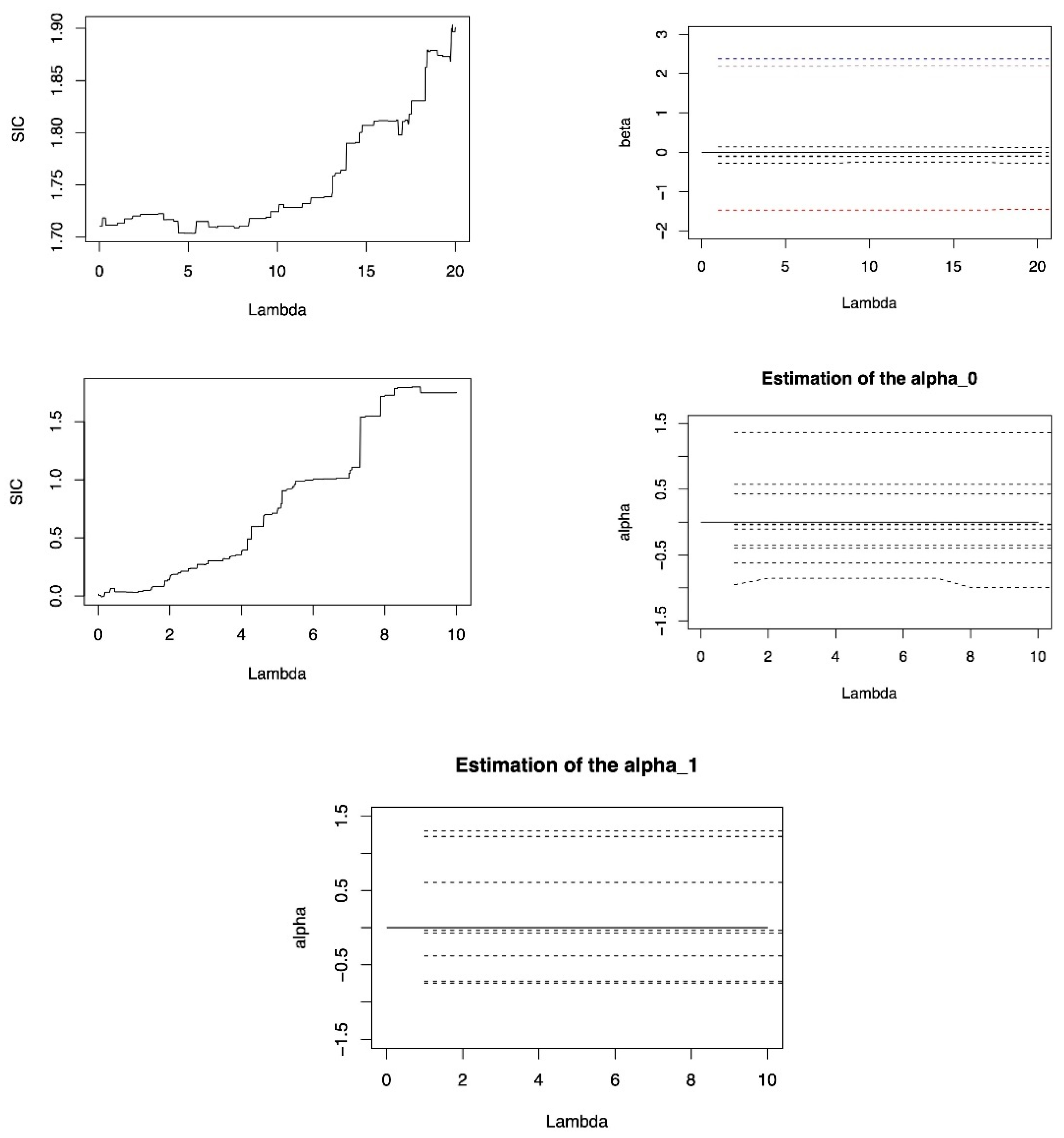
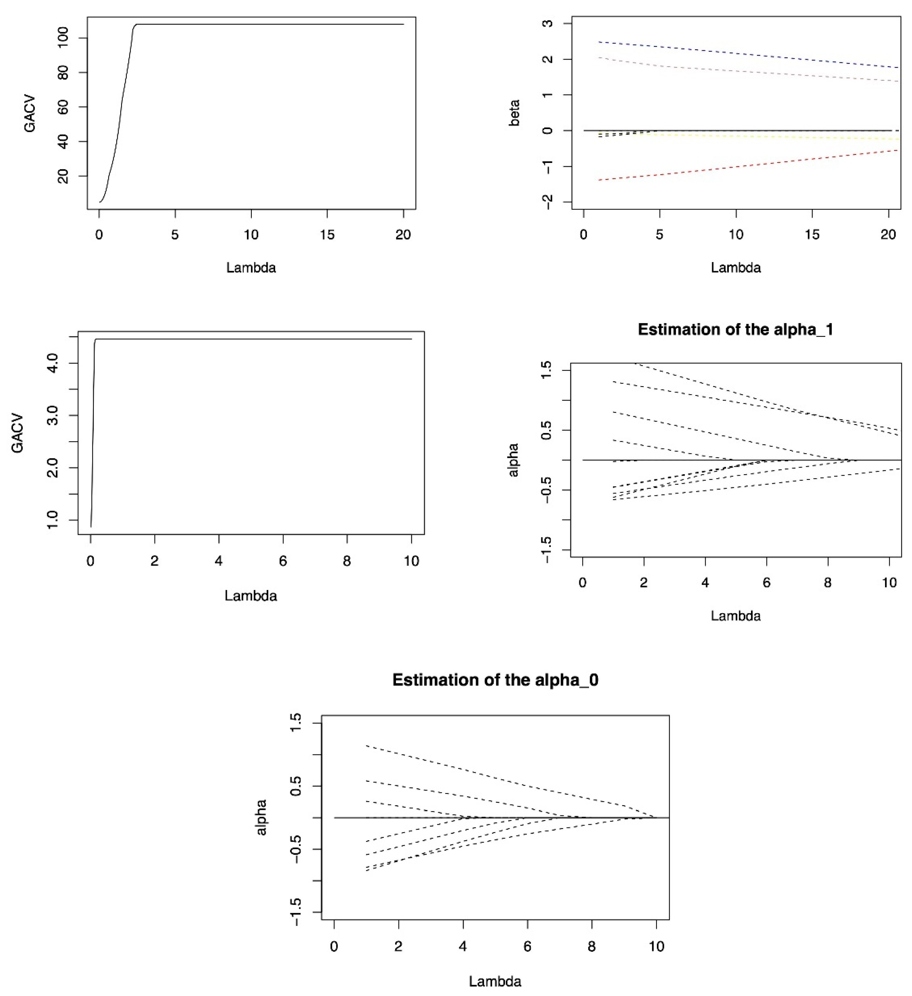
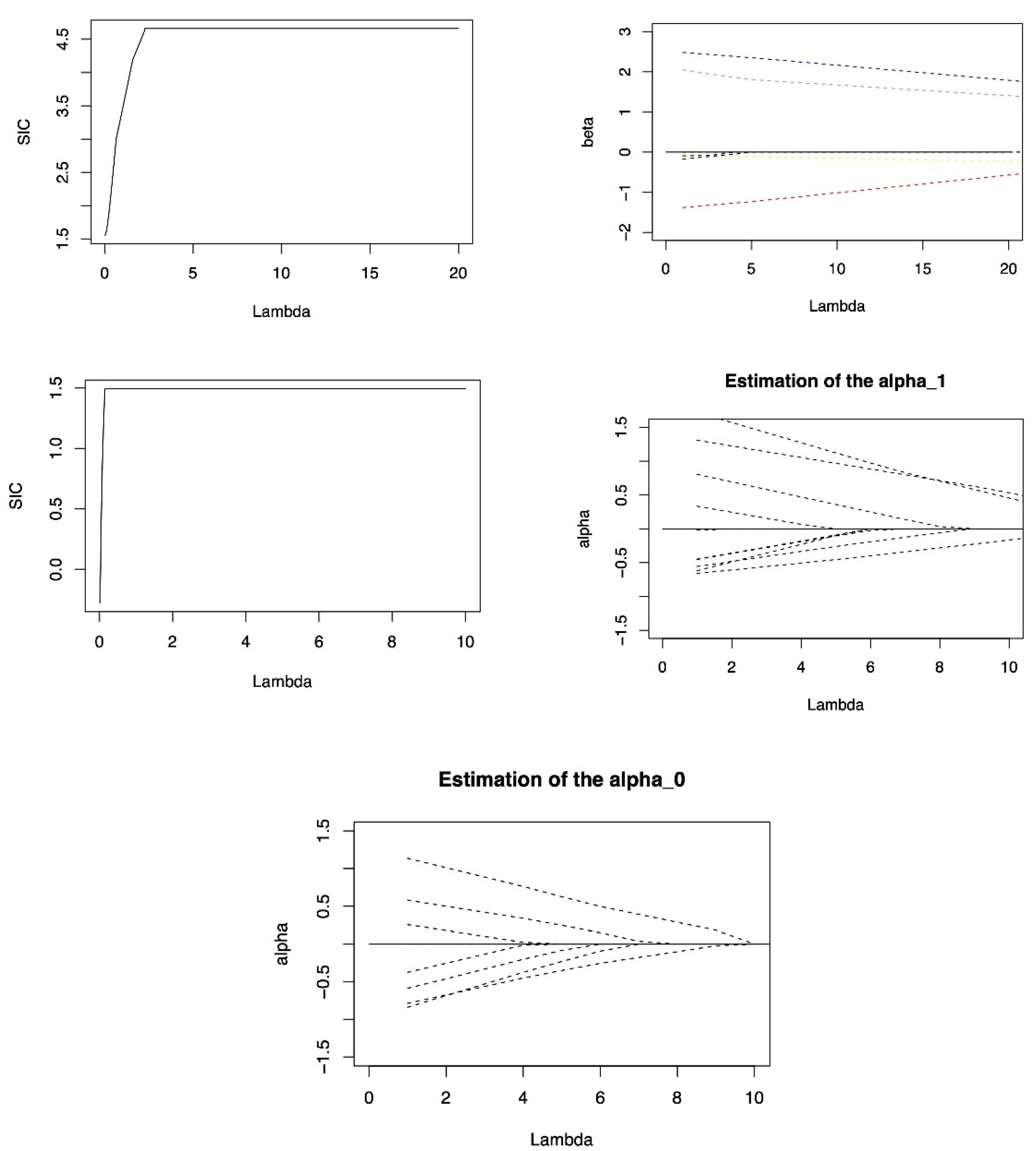
In this section, we illustrate the performance of the proposed double penalized expectile regression. In order to study the impact of the SIC criteria and the GACV criteria on double penalized Lasso expectile regression model and double penalized Lasso quantile regression model [9]. Simulation 1 is used to compare the two methods with different expectile levels and signal-to-noise ratio. And briefly denoted as DLER-SIC, DLER-GACV, DLQR-SIC, and DLQR-GACV; To illustrate the robustness of the DLER method in excluding inactive variables, simulation 2 and simulation 3 are given to study the impact of random effects on the coefficient estimation, comparing the performance of DLER and DLQR under different random effects. As well as comparing the obtained experimental values at different error distributions and different model sparsity to illustrate the advantage of DLER in variable selection; in order to illustrate the advantage of the DLER method in high-dimensional data, simulation 4 compares the two methods when dimensions of covariate is larger than the sample size.

In order to evaluate the accuracy of model coefficient estimation, we use mean square error (MSE) as the evaluation index. MSE is defined as:

$$MSE={\left({\widehat{\mathit{\beta }}}^t-\mathit{\beta }\right)}^{\mathrm{T}}{\Sigma }^{-1}\left({\widehat{\mathit{\beta }}}^t-\mathit{\beta }\right)$$

(14)

where $\Sigma ={\left({\rho }^{\left|k-h\right|}\right)}_{8\times 8}$, and ${\widehat{\mathit{\beta }}}^t$ is the estimator of $\mathit{\beta }$ in the $s\mathrm{th}$ simulation. SD stands for the 100-repetition Bootstrap standard deviation. Corr expresses the average proportion of important variables that were entered into the model correctly, and Incorr expresses the average proportion of inactive variables that were entered into the model incorrectly.$X_1(\mathrm{S}{\mathrm{D}}_1),X_2(\mathrm{S}{\mathrm{D}}_2),X_5(\mathrm{S}{\mathrm{D}}_5)$ represent the total number of choosing each important variable into the model correctly and its bootstrap standard deviation respectively. $X_3(\mathrm{S}{\mathrm{D}}_3),X_4(\mathrm{S}{\mathrm{D}}_4),X_6(\mathrm{S}{\mathrm{D}}_6),X_7(\mathrm{S}{\mathrm{D}}_7),X_8(\mathrm{S}{\mathrm{D}}_8)$ represent the total number of correctly excluded each redundant variable out of the model and its bootstrap standard deviation respectively. Int ($\mathrm{S}{\mathrm{D}}_{\mathrm{int}}$) represent the total number of choosing intercept into the model and its bootstrap standard deviation.

Simulation 1.

The impact of “signal-to-noise ratio” on estimation.

We compared the effectiveness of the two tuning parameter criteria, SIC and GACV. The process for producing the model data listed below was rated as

$$y_{ij}={\beta }_0+{\mathit{x}}_{ij}^{\mathrm{T}}\mathit{\beta }+{\mathit{z}}_{ij}^{\mathrm{T}}{\mathit{\alpha }}_i+\sigma r_{ij}$$

(15)

We let ${\mathit{x}}_{ij}^{\mathrm{T}}=\left(x_{ij1},x_{ij2},\cdots ,x_{ij8}\right)$, $i=1,2,\cdots ,20$, $j=1,2,\cdots ,25$,

${\mathit{Z}}_{ij}^{\mathrm{T}}=\left(x_{ij1},x_{ij2},\cdots ,x_{ij5}\right)$, and $X_1,\cdots ,X_8$ are generated from $N(0,1)$ with correlation between $X_k$ and $X_l$ being ${\rho }^{\left|l-k\right|}$, $\rho =0.5$. This paper sets the random effects are iid from ${\mathit{\alpha }}_i={\left({\alpha }_{i0},{\alpha }_{i1},\cdots ,{\alpha }_{i5}\right)}^{\mathrm{T}}\sim N_6\left(\mathbf{0},\mathit{P}\right)$, where $\mathit{P}=diag\left(1,1,1,1,0,0\right)$. And ${\beta }_0=0$, $\mathit{\beta }={\left(3,-1.5,0,0,2,0,0,0\right)}^{\mathrm{T}}$. The error terms are iid from $r_{ij}\sim N\left(0,1\right)$, we set $\tau =0.25,0.5,0.75$, and $\sigma =1,2,3$ to compare the estimation methods. In every simulation, we consider the estimator of coefficients to be 0 if its absolute value is less than 0.1. We set $\epsilon ={10}^{-3}$ in the iterative Lasso algorithm of DLER as the same settings in the iterative algorithm of DLQR of Li (2020) [8].

Table A1. The results 1 of simulation 1 under three signal-to-noise ratio.

Parameters	Method	MSE	$S{D}_{\mathbf{int}}$	$S{D}_1$	$S{D}_2$	$S{D}_3$	$S{D}_4$	$S{D}_5$	$S{D}_6$	$S{D}_7$	$S{D}_8$
$\tau =0.25$
$\sigma =1$	DLER-SIC	0.306	0.300	0.313	0.288	0.029	0.033	0.054	0.022	0.027	0.012
	DLER-GACV	0.486	0.303	0.411	0.383	0.027	0.035	0.056	0.024	0.035	0.025
	DLQR-SIC	0.280	0.261	0.297	0.250	0.060	0.046	0.091	0.015	0.024	0.020
	DLQR-GACV	0.289	0.266	0.299	0.254	0.063	0.049	0.088	0.037	0.039	0.031
$\sigma =2$	DLER-SIC	0.388	0.261	0.307	0.292	0.063	0.070	0.113	0.074	0.079	0.080
	DLER-GACV	0.490	0.266	0.371	0.342	0.066	0.069	0.113	0.085	0.084	0.078
	DLQR-SIC	0.527	0.234	0.332	0.335	0.108	0.088	0.167	0.076	0.069	0.086
	DLQR-GACV	0.535	0.236	0.333	0.324	0.110	0.098	0.169	0.083	0.086	0.084
$\sigma =3$	DLER-SIC	0.585	0.337	0.324	0.321	0.117	0.129	0.178	0.138	0.107	0.113
	DLER-GACV	0.649	0.342	0.330	0.343	0.139	0.133	0.186	0.139	0.128	0.110
	DLQR-SIC	0.868	0.341	0.337	0.375	0.162	0.162	0.244	0.134	0.165	0.117
	DLQR-GACV	0.894	0.353	0.325	0.398	0.163	0.163	0.244	0.153	0.152	0.119
$\tau =0.5$
$\sigma =1$	DLER-SIC	0.292	0.283	0.305	0.265	0.016	0.015	0.048	0.013	0.013	0
	DLER-GACV	0.509	0.283	0.438	0.342	0.015	0.019	0.049	0.014	0	0
	DLQR-SIC	0.207	0.242	0.262	0.224	0.026	0.022	0.083	0.015	0.015	0.017
	DLQR-GACV	0.219	0.240	0.256	0.231	0.032	0.038	0.093	0.029	0.026	0.032
$\sigma =2$	DLER-SIC	0.403	0.278	0.284	0.335	0.072	0.075	0.128	0.067	0.081	0.071
	DLER-GACV	0.472	0.276	0.320	0.359	0.076	0.074	0.133	0.065	0.069	0.063
	DLQR-SIC	0.424	0.273	0.262	0.325	0.088	0.095	0.160	0.079	0.058	0.073
	DLQR-GACV	0.464	0.272	0.269	0.324	0.095	0.097	0.167	0.086	0.075	0.091
$\sigma =3$	DLER-SIC	0.558	0.333	0.313	0.326	0.109	0.095	0.171	0.106	0.121	0.111
	DLER-GACV	0.634	0.334	0.323	0.338	0.129	0.125	0.179	0.134	0.126	0.115
	DLQR-SIC	0.673	0.317	0.300	0.346	0.119	0.135	0.216	0.122	0.106	0.114
	DLQR-GACV	0.720	0.320	0.311	0.361	0.118	0.129	0.218	0.133	0.121	0.121
$\tau =0.75$
$\sigma =1$	DLER-SIC	0.374	0.272	0.322	0.316	0.021	0.027	0.056	0.012	0.017	0
	DLER-GACV	0.456	0.275	0.389	0.369	0.025	0.020	0.058	0	0.021	0.007
	DLQR-SIC	0.307	0.275	0.320	0.255	0.054	0.027	0.105	0.024	0.023	0.028
	DLQR-GACV	0.321	0.275	0.318	0.260	0.070	0.039	0.097	0.031	0.039	0.041
$\sigma =2$	DLER-SIC	0.454	0.263	0.321	0.302	0.071	0.087	0.129	0.098	0.083	0.056
	DLER-GACV	0.538	0.262	0.400	0.359	0.072	0.086	0.124	0.106	0.070	0.064
	DLQR-SIC	0.547	0.251	0.319	0.309	0.097	0.117	0.187	0.093	0.060	0.070
	DLQR-GACV	0.570	0.255	0.317	0.317	0.103	0.117	0.198	0.099	0.081	0.078
$\sigma =3$	DLER-SIC	0.577	0.312	0.330	0.318	0.116	0.145	0.183	0.111	0.119	0.125
	DLER-GACV	0.617	0.309	0.347	0.336	0.130	0.146	0.187	0.116	0.123	0.115
	DLQR-SIC	0.701	0.283	0.336	0.322	0.119	0.137	0.246	0.131	0.129	0.129
	DLQR-GACV	0.770	0.304	0.329	0.348	0.121	0.153	0.247	0.154	0.150	0.157

and

Table A2. The results 2 of simulation 1 under three signal-to-noise ratio.

Parameters	Method	Corr (SD)	Incorr (SD)	Int	${\mathit{X}}_1$	${\mathit{X}}_2$	${\mathit{X}}_3$	${\mathit{X}}_4$	${\mathit{X}}_5$	${\mathit{X}}_6$	${\mathit{X}}_7$	${\mathit{X}}_8$
$\tau =0.25$
$\sigma =1$	DLER-SIC	3 (0)	1.04 (0.665)	14	100	100	95	95	100	97	96	99
	DLER-GACV	2.99 (0.1)	1.11 (0.751)	14	100	99	96	94	100	95	94	96
	DLQR-SIC	3 (0)	1.29 (0.518)	0	100	100	87	91	100	99	96	98
	DLQR-GACV	3 (0)	1.5 (0.628)	0	100	100	84	91	100	92	90	93
$\sigma =2$	DLER-SIC	3 (0)	1.6 (0.865)	1	100	100	90	88	100	88	88	85
	DLER-GACV	2.99 (0.1)	1.81 (0.982)	1	100	99	87	84	100	82	82	83
	DLQR-SIC	3 (0)	1.99 (0.959)	0	100	100	73	79	100	82	87	80
	DLQR-GACV	3 (0)	2.04 (1.063)	0	100	100	75	76	100	83	81	81
$\sigma =3$	DLER-SIC	3 (0)	1.87 (1.116)	0	100	100	85	83	100	83	79	83
	DLER-GACV	3 (0)	2.24 (1.311)	0	100	100	73	76	100	78	72	77
	DLQR-SIC	3 (0)	2.56 (1.351)	0	100	100	67	70	100	69	65	73
	DLQR-GACV	3 (0)	2.41 (1.280)	0	100	100	64	70	100	72	74	79
$\tau =0.5$
$\sigma =1$	DLER-SIC	3 (0)	0.75 (0.520)	29	100	100	99	99	100	99	99	100
	DLER-GACV	2.98 (0.2)	0.74 (0.525)	30	99	99	99	98	100	99	100	100
	DLQR-SIC	3 (0)	0.78 (0.645)	35	100	100	96	96	100	98	99	98
	DLQR-GACV	3 (0)	0.95 (0.770)	36	100	100	95	91	100	94	96	93
$\sigma =2$	DLER-SIC	2.99 (0.1)	1.37 (0.960)	29	100	99	89	87	100	86	85	87
	DLER-GACV	2.99 (0.1)	1.38 (1.080)	27	100	99	85	86	100	89	86	89
	DLQR-SIC	2.99(0.1)	1.66 (1.075)	27	100	99	78	78	100	83	88	80
	DLQR-GACV	2.99 (0.1)	1.76 (1.264)	31	100	99	76	78	100	79	81	79
$\sigma =3$	DLER-SIC	3 (0)	1.7 (1.124)	25	100	100	82	79	100	80	81	83
	DLER-GACV	3 (0)	1.98 (1.303)	28	100	100	74	71	100	73	78	78
	DLQR-SIC	3 (0)	2.38 (1.153)	22	100	100	66	69	100	62	72	71
	DLQR-GACV	3 (0)	2.22 (1.211)	20	100	100	70	69	100	74	70	75
$\tau =0.75$
$\sigma =1$	DLER-SIC	2.99 (0.1)	0.94 (0.528)	15	100	99	98	96	100	99	98	100
	DLER-GACV	2.99 (0.1)	0.96 (0.470)	14	100	99	96	98	100	100	97	99
	DLQR-SIC	3 (0)	1.29 (0.478)	0	100	100	87	96	100	96	98	94
	DLQR-GACV	3 (0)	1.47 (0.717)	0	100	100	80	94	100	94	93	92
$\sigma =2$	DLER-SIC	3 (0)	1.72 (0.877)	0	100	100	88	84	100	82	86	88
	DLER-GACV	2.99 (0.1)	1.84 (1.042)	1	100	99	83	85	100	75	88	84
	DLQR-SIC	3 (0)	2.04 (0.974)	0	100	100	78	72	100	71	92	83
	DLQR-GACV	3 (0)	2.12 (1.113)	0	100	100	74	75	100	75	85	79
$\sigma =3$	DLER-SIC	3 (0)	1.93 (1.066)	0	100	100	87	80	100	83	82	75
	DLER-GACV	3 (0)	2.16 (1.245)	0	100	100	78	77	100	78	76	75
	DLQR-SIC	3 (0)	2.44 (1.192)	0	100	100	72	69	100	70	72	73
	DLQR-GACV	3 (0)	2.62 (1.237)	0	100	100	67	70	100	69	68	64

(in the Appendix C) give the results of coefficient estimation and variable selection, respectively.

According to Table A1, the estimation accuracy of the model is first analyzed. When $\sigma$ is fixed, the MSE of the two methods is almost reaches the minimum at $\tau =0.5$, the estimation accuracy of the two methods is better, while the accuracy at the other fractile is slightly worse, but the difference is not obvious, for example when $\sigma =1$, MSE of DLER-SIC method is 0.292 at $\tau =0.5$, while at the other expectile levels are 0.306 and 0.374, respectively. In this case, this shows that the DLER method has the same accuracy as the DLQR method in parameter estimation. In addition, according to the results of the two tunning parameter criterions, the estimation accuracy under the SIC is better than the GACV whether the DLER model or the DLQR model.

Next, analyze the accuracy of variable selection. According to the SD of each variable estimation in Table A1, when fixed $\sigma$, with the increase of $\tau$, SD decreases gradually, and the accuracy of variable selection of the two models is gradually increased. For each important variable, according to Table A2, the DLER method can select 99% of the important variables into the model. In addition, for each inactive variable, comparing the results in the table, shows that when $\tau$ is fixed, with the increase of $\sigma$, the SD is also increasing, indicating that the accuracy of DLQR method is gradually weakened in excluding inactive variables out of the model. For DLER method, the SD is the largest at $\sigma =2$, DLER method has the low accuracy, it is still better than DLQR at this time, especially at $\sigma =3$, the SD is the smallest, indicating that with the increase of signal-to-noise ratio, DLER method is better than DLQR method in excluding the redundant variables. Combined with the results of Table A2, the same conclusion can be obtained.

Therefore, for the parameter estimation of the methods, when the signal-to-noise ratio with relatively large, the DLER method is better than the DLQR method. In terms of model variables selection, whether in SIC and GACV criteria, almost 99%of important variables can be selected in both methods. For the ability to exclude the redundant variables, the DLER method is more advantageous than the DLQR method. Therefore, in terms of the accuracy of parameter estimation, DLER method and DLQR method have the same effect. However, the DLER method is better than the DLQR method in terms of estimated stability and excluding inactive variables.

Simulation 2.

The influence of random effects.

We use the simulation to show the influence of random effects on DLER-SIC, DLER-GACV, DLQR-SIC and DLQR-GACV. The data generation model is Equation (15) with the fixed $\sigma =1$. And consider the covariance matrix of the random effect $\mathit{P}$ with three forms:

$${\mathit{P}}_1=\mathrm{diag}\left(1,1,1,1,0,0\right)$$

$${\mathit{P}}_2=\mathrm{diag}\left(2,2,2,2,0,0\right)$$

$${\mathit{P}}_3=\mathrm{diag}\left(3,3,3,3,0,0\right)$$

With the increasing of random effects, we get the results of 100 repetitions simulations with $\tau =0.25,0.5,0.75$.

Table A3. The results 1 of simulation 2 under different influence of random effects.

$\tau =0.5$	Method	MSE	$S{\mathrm{D}}_{\mathbf{int}}$	$S{\mathrm{D}}_1$	$S{\mathrm{D}}_2$	$S{\mathrm{D}}_3$	$S{\mathrm{D}}_4$	$S{\mathrm{D}}_5$	$S{\mathrm{D}}_6$	$S{\mathrm{D}}_7$	$S{\mathrm{D}}_8$
${\mathit{P}}_1$
	DLER-SIC	0.336	0.268	0.314	0.281	0.016	0.012	0.054	0.022	0.010	0.026
	DLER-GACV	0.490	0.266	0.409	0.321	0.019	0.017	0.057	0.021	0.016	0.019
	DLQR-SIC	0.286	0.229	0.294	0.279	0.051	0.037	0.079	0.030	0.021	0.018
	DLQR-GACV	0.294	0.233	0.298	0.276	0.056	0.043	0.085	0.038	0.034	0.031
${\mathit{P}}_2$
	DLER-SIC	1.318	0.539	0.559	0.568	0.013	0	0.049	0.021	0.014	0.012
	DLER-GACV	2.231	0.538	0.789	0.574	0.020	0	0.051	0.020	0.013	0.011
	DLQR-SIC	0.898	0.520	0.534	0.508	0.045	0.478	0.099	0.022	0.026	0
	DLQR-GACV	0.916	0.517	0.528	0.516	0.052	0.049	0.107	0.041	0.037	0.018
${\mathit{P}}_3$
	DLER-SIC	2.577	0.876	0.906	0.726	0.022	0.024	0.049	0	0.017	0.022
	DLER-GACV	3.946	0.879	1.065	0.733	0.015	0.018	0.052	0.014	0.013	0.012
	DLQR-SIC	1.869	0.732	0.793	0.746	0.040	0.092	0.108	0.027	0.011	0.010
	DLQR-GACV	1.878	0.727	0.803	0.760	0.050	0.099	0.076	0.027	0.019	0.020

and

Table A4. The results 2 of simulation 2 with different influence of random effects.

$\tau =0.5$	Method	Corr (SD)	Incorr (SD)	Int	${\mathit{X}}_1$	${\mathit{X}}_2$	${\mathit{X}}_3$	${\mathit{X}}_4$	${\mathit{X}}_5$	${\mathit{X}}_6$	${\mathit{X}}_7$	${\mathit{X}}_8$
${\mathit{P}}_1$
	DLER-SIC	3 (0)	0.8 (0.651)	29	100	100	98	99	100	98	99	97
	DLER-GACV	3 (0)	0.81 (0.598)	29	100	100	98	98	100	98	98	98
	DLQR-SIC	3 (0)	1.03 (0.643)	30	100	100	85	93	100	94	97	98
	DLQR-GACV	3 (0)	1.17 (0.877)	28	100	100	85	90	100	91	94	95
${\mathit{P}}_2$
	DLER-SIC	2.91 (0.288)	0.98 (0.376)	9	100	91	99	100	100	97	98	99
	DLER-GACV	2.78 (0.462)	0.99 (0.362)	8	98	80	98	100	100	98	98	99
	DLQR-SIC	3 (0)	1.12 (0.591)	15	15	100	90	90	100	98	96	100
	DLQR-GACV	3 (0)	1.24 (0.754)	17	17	100	87	90	100	91	93	98
${\mathit{P}}_3$
	DLER-SIC	2.75 (0.435)	1.04 (0.470)	6	99	76	98	98	100	100	98	96
	DLER-GACV	2.46 (0.673)	1.01 (0.460)	7	90	56	99	98	100	99	98	98
	DLQR-SIC	2.97 (0.171)	1.11 (0.601)	15	100	100	93	87	100	96	99	99
	DLQR-GACV	2.97 (0.171)	1.24 (0.605)	4	100	100	87	84	100	96	98	97

(in the Appendix C) give the results of estimation and variable selection of different methods under different random effects at $\mathit{\tau }=0.5$.

According to Table A3, with the increasing interference of random effects, although the estimation accuracy of the two methods is decreasing, and the accuracy of the fixed effect coefficient is decreasing, especially the first two important covariates interfered by random effects. However, in term of variable selection, DLER method has little change in the accuracy of variable selection, and almost all the important variables can be choosing into the model, and the ability to exclude the inactive variables is still better than DLQR method. In particular, the DLER-SIC method, combined with Table A4, shows that the proportion of correctly choosing variables is 99%, and the accuracy of excluding the redundant variables is almost above 90%. In general, since the double penalized expectile regression takes into account the random effects while selecting fixed effects, it can be almost free from the interference of random effects in the accuracy of variables selection, but it will still be affected by random effects to a degree in the accuracy of fixed effect coefficient estimation. Therefore, in terms of the accuracy of parameter estimation, DLER method and DLQR method have the same effect. However, DLER is still more robust than DLQR in variable selection, even if the interference of random effects is added to the model.

Simulation 3.

The case of different model sparsity and error distribution.

We compare DLQR and DLER under different model sparsity and error distribution. The data generation model is Equation (15), considering the fixed effect as the following three cases

(1)

Dense $\mathit{\beta }={\left(1,1,1,1,1,1,1,1\right)}^{\mathrm{T}}$

(2)

Sparse $\mathit{\beta }={\left(3,1.5,0,0,2,0,0,0\right)}^{\mathrm{T}}$

(3)

High Sparse $\mathit{\beta }={\left(5,0,0,0,0,0,0,0\right)}^{\mathrm{T}}$

We consider $\sigma =1$, $\tau =0.5$, $\mathit{P}=\mathrm{diag}\left(2,2,2,2,0,0\right)$, the distribution of error term respectively comes form $N\left(0,1\right)$, $t\left(3\right)$ and $Cauchy\left(0,1\right)$. Comparing the models DLER-SIC, DLER-GACV, DLQR-SIC and DLQR-GACV. Tables shows the results of the three models by 100 repetitions simulations.

Table A5. The results 1 of simulation 3 with dense model under different error distributions.

Model	Method	MSE	$S{\mathrm{D}}_{\mathrm{int}}$	$S{\mathrm{D}}_1$	$S{\mathrm{D}}_2$	$S{\mathrm{D}}_3$	$S{\mathrm{D}}_4$	$S{\mathrm{D}}_5$	$S{\mathrm{D}}_6$	$S{\mathrm{D}}_7$	$S{\mathrm{D}}_8$
Dense
$N\left(0,1\right)$	DLER-SIC	0.908	0.522	0.544	0.527	0.058	0.061	0.066	0.068	0.058	0.053
	DLER-GACV	0.922	0.522	0.558	0.550	0.058	0.062	0.066	0.068	0.059	0.053
	DLQR-SIC	0.853	0.468	0.485	0.527	0.079	0.079	0.081	0.093	0.076	0.070
	DLQR-GACV	0.882	0.463	0.476	0.536	0.088	0.086	0.087	0.102	0.084	0.073
$t\left(3\right)$	DLER-SIC	0.965	0.556	0.570	0.534	0.140	0.097	0.104	0.113	0.108	0.113
	DLER-GACV	1.114	0.551	0.560	0.590	0.187	0.114	0.125	0.126	0.131	0.163
	DLQR-SIC	0.871	0.518	0.525	0.467	0.113	0.099	0.101	0.118	0.108	0.094
	DLQR-GACV	0.872	0.520	0.520	0.484	0.115	0.095	0.088	0.113	0.103	0.095
$Cauchy\left(0,1\right)$	DLER-SIC	4.397	0.391	0.404	0.678	0.105	0.272	0.391	0.370	0.753	0.377
	DLER-GACV	4.828	0.535	0.405	0.795	0.306	0.310	0.397	0.370	0.725	0.424
	DLQR-SIC	2.450	0.249	0.350	0.605	0.039	0.089	0.031	0.072	0.092	0.127
	DLQR-GACV	2.157	0.237	0.361	0.555	0.008	0.0536	0.041	0.020	0.094	0.129

and

Table A6. The results 2 of simulation 3 with dense model under different error distributions.

Model	Method	Corr (SD)	Incorr (SD)	Int	${\mathit{X}}_1$	${\mathit{X}}_2$	${\mathit{X}}_3$	${\mathit{X}}_4$	${\mathit{X}}_5$	${\mathit{X}}_6$	${\mathit{X}}_7$	${\mathit{X}}_8$
Dense
$N\left(0,1\right)$	DLER-SIC	7.99 (0.33)	0.74 (0.44)	26	94	96	100	100	100	100	100	100
	DLER-GACV	7.7 (0.63)	0.74 (0.44)	26	84	86	100	100	100	100	100	100
	DLQR-SIC	7.9 (0.33)	0.78 (0.42)	22	94	96	100	100	100	100	100	100
	DLQR-GACV	7.91 (0.32)	0.81 (0.39)	19	96	95	100	100	100	100	100	100
$t\left(3\right)$	DLER-SIC	7.72 (0.62)	0.84 (0.37)	16	83	90	99	100	100	100	100	100
	DLER-GACV	7.37 (0.92)	0.83 (0.38)	17	66	73	99	100	100	100	100	99
	DLQR-SIC	7.88 (0.33)	0.84 (0.37)	16	93	95	100	100	100	100	100	100
	DLQR-GACV	7.91 (0.29)	0.84 (0.37)	16	95	96	100	100	100	100	100	100
$Cauchy\left(0,1\right)$	DLER-SIC	7.6 (0.80)	0.8 (0.40)	20	100	100	100	100	80	80	100	100
	DLER-GACV	7.68 (0.47)	1 (0)	0	100	100	100	100	88	80	100	100
	DLQR-SIC	8 (0)	0.8 (0.40)	20	100	100	100	100	100	100	100	100
	DLQR-GACV	8 (0)	0.8 (0.40)	20	100	100	100	100	100	100	100	100

show the results of coefficient estimation and variable selection under the dense model,

Table A7. The results 1 of simulation 3 with the sparse model under different error distributions.

Model	Method	MSE	$S{D}_{\mathbf{int}}$	$S{D}_1$	$S{D}_2$	$S{D}_3$	$S{D}_4$	$S{D}_5$	$S{D}_6$	$S{D}_7$	$S{D}_8$
Sparse
$N\left(0,1\right)$	DLER-SIC	1.345	0.608	0.622	0.550	0.011	0	0.051	0.015	0.015	0.023
	DLER-GACV	2.084	0.608	0.849	0.606	0.011	0	0.052	0.019	0.014	0.018
	DLQR-SIC	0.978	0.508	0.527	0.544	0.030	0.033	0.123	0.030	0.020	0.013
	DLQR-GACV	0.947	0.516	0.527	0.529	0.036	0.037	0.106	0.037	0.028	0.027
$t\left(3\right)$	DLER-SIC	1.230	0.676	0.533	0.605	0.055	0.039	0.104	0.075	0.049	0.064
	DLER-GACV	2.737	0.670	1.083	0.742	0.070	0.053	0.204	0.082	0.057	0.075
	DLQR-SIC	1.008	0.522	0.498	0.530	0.065	0.049	0.102	0.041	0.047	0.048
	DLQR-GACV	1.000	0.529	0.492	0.531	0.066	0.055	0.106	0.046	0.047	0.049
$Cauchy\left(0,1\right)$	DLER-SIC	5.756	0.620	0.732	0.404	0.121	0	0.399	0.587	0.238	0.385
	DLER-GACV	6.791	0.708	0.753	0.307	0.384	0.073	0.542	0.682	0.521	0.460
	DLQR-SIC	2.099	0.593	0.411	0.310	0.105	0.193	0.152	0.119	0.046	0.062
	DLQR-GACV	1.758	0.638	0.385	0.342	0	0.173	0.113	0.095	0.049	0.034

and

Table A8. The results 2 of simulation 3 with the sparse model under different error distributions.

Model	Method	Corr (SD)	Incorr (SD)	Int	${\mathit{X}}_1$	${\mathit{X}}_2$	${\mathit{X}}_3$	${\mathit{X}}_4$	${\mathit{X}}_5$	${\mathit{X}}_6$	${\mathit{X}}_7$	${\mathit{X}}_8$
Sparse
$N\left(0,1\right)$	DLER-SIC	2.91 (0.288)	0.98 (0.40)	8	100	91	99	100	100	99	98	98
	DLER-GACV	2.79 (0.478)	0.98 (0.40)	8	97	82	99	100	100	97	99	99
	DLQR-SIC	3 (0)	1.09 (0.62)	14	100	100	94	92	100	95	97	99
	DLQR-GACV	3 (0)	1.17 (0.63)	14	100	100	94	92	100	92	95	96
$t\left(3\right)$	DLER-SIC	2.94 (0.24)	1.38 (0.84)	8	100	94	91	96	100	87	93	87
	DLER-GACV	2.59 (0.71)	1.55 (1.06)	12	87	72	84	91	100	83	90	85
	DLQR-SIC	2.97 (0.17)	1.27 (0.79)	15	100	97	88	91	100	92	94	93
	DLQR-GACV	2.97 (0.17)	1.38 (0.85)	16	100	97	86	86	100	90	93	91
$Cauchy\left(0,1\right)$	DLER-SIC	2.84 (0.37)	2.02 (0.62)	0	100	84	79	100	100	80	59	80
	DLER-GACV	3 (0)	4.62 (0.83)	7	100	100	2	78	100	18	15	18
	DLQR-SIC	3 (0)	2.66 (1.11)	0	100	100	79	36	100	71	71	77
	DLQR-GACV	3 (0)	2.09 (0.93)	0	100	100	100	43	100	71	84	93

show the results under the sparse model,

Table A9. The results 1 of simulation 3 with the high sparse model under different error distributions.

Model	Method	MSE	$S{D}_{\mathbf{int}}$	$S{D}_1$	$S{D}_2$	$S{D}_3$	$S{D}_4$	$S{D}_5$	$S{D}_6$	$S{D}_7$	$S{D}_8$
High Sparse
$N\left(0,1\right)$	DLER-SIC	1.017	0.611	0.593	0.267	0.020	0.021	0.025	0.039	0.035	0.017
	DLER-GACV	3.096	0.613	0.981	0.253	0.017	0.022	0.025	0.033	0.016	0
	DLQR-SIC	0.773	0.523	0.493	0.475	0.038	0.029	0.030	0.020	0.018	0.035
	DLQR-GACV	0.81	0.528	0.509	0.477	0.048	0.040	0.036	0.039	0.041	0.036
$t\left(3\right)$	DLER-SIC	1.264	0.528	0.73	0.282	0.055	0	0.024	0.042	0.083	0.091
	DLER-GACV	2.478	0.519	1.019	0.307	0.069	0.039	0.03	0.039	0.092	0.087
	DLQR-SIC	0.792	0.474	0.576	0.394	0.082	0.072	0.051	0.061	0.036	0.039
	DLQR-GACV	0.777	0.483	0.575	0.374	0.056	0.054	0.047	0.038	0.029	0.035
$Cauchy\left(0,1\right)$	DLER-SIC	1.925	1.147	0.162	0.741	0	0.513	0	0	0	0.371
	DLER-GACV	14.720	1.200	0.298	1.289	0.932	1.201	0.602	0.513	0.227	0.334
	DLQR-SIC	0.798	0.650	0.256	0.484	0.117	0.095	0.082	0.029	0.124	0.121
	DLQR-GACV	0.822	0.567	0.238	0.415	0.116	0.088	0.060	0.0315	0.109	0.109

and

Table A10. The results 2 of simulation 3 with the high sparse model under different error distributions.

Model	Method	Corr (SD)	Incorr (SD)	Int	${\mathit{X}}_1$	${\mathit{X}}_2$	${\mathit{X}}_3$	${\mathit{X}}_4$	${\mathit{X}}_5$	${\mathit{X}}_6$	${\mathit{X}}_7$	${\mathit{X}}_8$
High Sparse
$N\left(0,1\right)$	DLER-SIC	1 (0)	1.43 (0.78)	4	100	75	98	98	98	92	95	97
	DLER-GACV	1 (0)	1.27 (0.72)	4	100	83	98	98	98	94	98	100
	DLQR-SIC	1 (0)	1.59 (0.78)	29	100	35	93	97	95	99	98	95
	DLQR-GACV	1 (0)	1.71 (0.97)	31	100	39	92	92	94	95	92	94
$t\left(3\right)$	DLER-SIC	1 (0)	1.52 (0.92)	2	100	75	91	100	98	94	93	95
	DLER-GACV	0.99 (0.1)	1.7 (1.11)	2	99	70	87	94	96	96	94	91
	DLQR-SIC	1 (0)	2.25 (1.22)	14	100	34	78	84	89	90	94	92
	DLQR-GACV	1 (0)	1.94 (1.08)	11	100	45	85	90	90	95	96	94
$Cauchy\left(0,1\right)$	DLER-SIC	1 (0)	1.71 (0.76)	0	100	82	100	53	100	100	100	94
	DLER-GACV	1 (0)	6.53 (2.35)	0	100	11	12	11	29	30	30	24
	DLQR-SIC	1 (0)	3.93 (1.28)	6	100	6	40	68	54	99	67	67
	DLQR-GACV	1 (0)	3.06 (1.54)	6	100	48	39	68	96	99	67	71

show the results under the highly sparse model. (See Appendix C for tables).

According to Table A5. At this time, all variables are important variables. With the change of error distribution, MSE are increasing, and the estimation accuracy of the two methods are decreased. We find that DLER method and DLQR method have the same effect in term of the accuracy of parameter estimation. In addition, considering the accuracy of variable selection of the two methods. Although the two methods cannot completely choose all the important variables into the model, it can be known from Table A6 that the average of the correct variables retained by them is more than 7.6, which is very close to the true value 8. Moreover, when the error term is adjusted from the normal distribution to the heavy-tailed distribution, the change of DLER is the smallest in all methods, so it is weak on the influence of different error distributions. In summary, DLER is robust to the change of error distribution on variable selection.

Next, the results of sparse model and highly sparse model are analyzed. Firstly, the estimation accuracy of DLER method and DLQR method is analyzed. The results are similar to the dense model, with the error distribution becoming more complex, MSE are increasing, and the estimation accuracy of the two methods is decreased. Next, considering the accuracy of the variable selection in model, according to Table A7 and Table A8, when the error obeys the normal distribution, for the sparse model, the two methods have little difference in the accuracy of excluding the inactive variables. However, when the error obeys distribution $t\left(3\right)$ or $Cauchy\left(0,1\right)$, the DLER method is significantly better than DLQR. Especially in the highly sparse model with error distribution $Cauchy\left(0,1\right)$, DLER excluding the inactive variables advantage is more obvious, especially DLER-SIC method. It shows that expectile regression is quite robust than quantile regression.

Simulation 4.

The case of high dimensional data.

High-dimensional data is widely available in the stock exchange market, biomedicine, aerospace and other fields, so the modeling and analysis of high-dimensional data has very important practical significance. Next, we investigate the performance of the proposed model in the high-dimensional scenarios of selecting variables. The data generation model is still the Equation (15), we reduce the sample size to $n=10$, $m=10$, that is, the total sample size is 100. In addition, 102 independent noise variables $X_9,X_{10},\cdots ,X_{110}$ are added to the above sparse model, all variables are independent and identically distributed in $N\left(0,{0.25}^2\right)$, thus the total number of variables is 110, larger than the total sample size, and ${\mathit{\beta }}_{110\times 1}=(3,1.5,0,0,2,0,0,0,\cdots {,0)}^{\mathrm{T}}$. There are three real important covariates and 107 redundant covariates. In addition, we set $\sigma =0.5$, $\mathit{P}=\mathrm{diag}\left(1,1,1,1,0,0\right)$.

Table A11. The results 1 of simulation 4 with the high dimensional model.

Model	Method	MSE	$S{D}_0$	$S{D}_1$	$S{D}_2$	$S{D}_5$
$\tau =0.5$
	DLER-SIC	4.783	0.010	0.513	0.360	0.657
	DLER-GACV	5.414	0.007	0.914	0.482	0.706
	DLQR-SIC	39.235	0.406	0.585	0.606	0.443
	DLQR-GACV	6.902	0.003	0.876	0.463	0.789
$\tau =0.75$
	DLER-SIC	5.870	0.165	0.671	0.383	0.882
	DLER-GACV	4.483	0.010	0.759	0.467	0.719
	DLQR-SIC	40.62433	0.413	0.593	0.625	0.507
	DLQR-GACV	7.799	0.009	0.916	0.514	0.723

and

Table A12. The results 2 of simulation 4 with the high dimensional model.

Model	Method	Corr (SD)	Incorr (SD)	${\mathit{X}}_0$	${\mathit{X}}_1$	${\mathit{X}}_2$	${\mathit{X}}_5$
$\tau =0.5$
	DLER-SIC	2.34 (0.590)	5.31 (2.237)	95.953	100	44	90
	DLER-GACV	2.28 (0.805)	3.46 (1.904)	97.682	88	50	90
	DLQR-SIC	3 (0)	94.3 (3.033)	12.794	100	100	100
	DLQR-GACV	2.8 (0.426)	68.44 (33.202)	36.972	98	91	91
$\tau =0.75$
	DLER-SIC	2.27 (0.737)	5.54 (7.885)	95.738	96	53	78
	DLER-GACV	2.58 (0.684)	5.32 (3.490)	95.963	96	72	90
	DLQR-SIC	2.99 (0.1)	94.46 (3.963)	12.654	100	100	99
	DLQR-GACV	2.68 (0.490)	42.06 (41.702)	61.617	98	82	88

(in the Appendix C) show 100 repeated results of the two methods at $\tau =0.5,0.75$, where $X_0$($S{\mathbf{D}}_0$) denote the average and bootstrap standard deviation of all redundant variables being correctly excluded out of the model.

Firstly, analyze the estimation precision of the two methods. According to Table A11, in the situation of fixed quantile, when the dimension of covariates is larger than the sample size, the MSE is larger than the previous simulation, the change of the MSE value of the DLER method is less than DLQR, and the MSE of the DLQR method is significantly larger than the DLER, indicating that although the estimation accuracy of the two methods is decreasing, the DLER method is significantly better than the DLQR method, and the stability of the DLER method is better than the DLQR method. Next, analyze the accuracy of variable selection. According to Table A11 and Table A12, the DLER method can ensure that the proportion of excluding redundant variables is more than 95% under three expectile levels. When the expectile level is fixed, DLER method has absolute advantages over DLQR in excluding redundant variables, especially DLER-GACV method can exclude more than 97% of the inactive variables at $\tau =0.5$. Therefore, when the dimension of covariates is larger than the sample size, DLER method is superior to DLQR in terms of estimation accuracy and excluding the inactive variables both at median $\tau =0.5$ and extreme expectile level $\tau =0.75$.

5. Application

CD4 cells play an important role in determining the efficacy of AIDS treatment and the immune function of patients, so excluding inactive variables is important for analyzing CD4 cell data. We applied the model to the real data of CD4 cell count. For a complete description of the data set, please refer to Diggle P.J’ s homepage: https://www.lancaster.ac.uk/staff/diggle/, accessed on 30 June 2022, and we select a part of this data set. The response variable is the open-root conversion of CD4 cell count. The variables in the data set include the time of seroconversion (time), the age relative to a starting point (age), the smoking status depicted by the number of packets smoked (smoking), the number of sexual partners (sex partner), and the depression state and depression degree (depression). Choosing time, smoking, age and sex partner as important fixed effect to determine the CD4 cell numbers, where time and age are important random effects. On this basis, consider the following model:

$${\mathit{Y}}_{ij}={\mathit{X}}_{ij}^{\mathrm{T}}\mathit{\beta }+{\mathit{Z}}_{ij}^{\mathrm{T}}{\mathit{\alpha }}_i+r_{ij}$$

where ${\mathit{Y}}_{ij}$ is the $j\mathrm{th}$ observation of the ith individual, ${\mathit{X}}_{ij}^{\mathrm{T}}$ is the observation of explanatory variables, and ${\mathit{Z}}_{ij}^{\mathrm{T}}$ is a subset of ${\mathit{X}}_{ij}^{\mathrm{T}}$. We set that the threshold of $\mathit{\beta }$ is 0.05, and the threshold of ${\mathit{\alpha }}_i$ is 0.1.

Table A13. CD4 cell data: the estimation of DLER-SIC, DLER-GACV, DLQR-SIC, DLQR-GACV.

	Int	Time ${\mathit{X}}_1$	Smoking ${\mathit{X}}_2$	Age ${\mathit{X}}_3$	Sex Partner ${\mathit{X}}_4$
$\tau =0.1$
DLER-SIC	−0.255	−0.271	0.080	0	0
DLER-GACV	−0.190	−0.266	0.058	0	0
DLQR-SIC	−0.851	−0.314	0.117	0	0
DLQR-GACV	−0.852	−0.313	0.119	0	0
$\tau =0.25$
DLER-SIC	−0.047	−0.243	0.080	0	0
DLER-GACV	0	−0.234	0.051	0	0
DLQR-SIC	−0.422	−0.258	0.117	0	0
DLQR-GACV	−0.420	−0.259	0.123	0	0
$\tau =0.5$
DLER-SIC	0.129	−0.233	0.090	0	0
DLER-GACV	0.112	−0.241	0.101	0	0
DLQR-SIC	0.126	−0.208	0.113	0	0
DLQR-GACV	0.126	−0.207	0.105	0	0
$\tau =0.75$
DLER-SIC	0.345	−0.220	0.074	0	0
DLER-GACV	0.329	−0.230	0.098	0	0
DLQR-SIC	0.557	−0.167	0.104	0	0
DLQR-GACV	0.559	−0.166	0.129	0	0
$\tau =0.9$
DLER-SIC	0.492	−0.217	0.078	0	0
DLER-GACV	0.492	−0.228	0.093	0	0
DLQR-SIC	0.959	−0.141	0.154	0	0
DLQR-GACV	0.949	−0.14	0.153	0	0

(in the Appendix C) gives the results of the four methods at $\tau =0.1,0.25,0.5,0.75,0.9$.

From the results of Table A13, the double penalized expectile regression method proposed can give the results of variable selection while estimating the coefficients. The variable with a value of 0 in the table indicates that it can be excluded from the model. It can be found that both estimation methods excluded variables $X_3$ and $X_4$ from the model. In the four variables, only time and smoking will affect CD4 cells. From the sign of coefficient estimation, the value of time is always less than 0, indicating that time has a negative influence on CD4 cells. The values of smoking are all larger than 0, indicating that smoking has a positive influence on CD4 cells.

Analysis of the numerical changes. For variable $X_2$, under the SIC criterion, with the changes of expectile level, the DLER method fluctuates less, and the DLER is relatively stable. Indicating that the stability of the DLER-SIC method is slightly stronger. For variable $X_1$, whether it is the SIC criteria or the GACV criteria, the numerical fluctuation of the DLER method is less than the DLQR method, indicating that the stability of DLER for estimation of variable $X_1$ is better than that of DLOR.

This shows that DLER method has strong practical utility for CD4 data in excluding inactive variables and analyzing its influencing factors.

6. Conclusions

In this paper, we propose the double penalized expectile regression method for linear mixed effects model, which imposes penalties on both fixed effects and random effects, fully accounting for the random effects in coefficient variable selection and estimation. The model proposed in this paper is found to be highly robust in excluding inactive variables after simulations and application studies. The conclusion is also supported by comparison with double penalized quantile regression method, through the comparison of the results of the two estimation methods, it can be found that the double penalized expectile regression has the same effect as the double penalized quantile regression in term of the accuracy of parameter estimation, but has absolute advantage in selecting variables, especially in excluding inactive variables.

When the signal-to-noise ratio is different, the precision of coefficient estimation and the accuracy of variable selection will be different. When the signal-to-noise ratio is larger, the proposed method outperforms the quantile model in terms of coefficient estimation ability and excluding inactive variables. In addition, because the double penalized expectile regression select variable for both fixed and mixed effects, it is almost undisturbed to random effects in terms of variable selection accuracy. When comparing the dense and sparse models, it is found that the sparser the model and the more complex the error term distribution, the advantage of the new method is more obvious, indicating that it has strong robustness. When the dimension of covariates is larger than the sample size, the method has obvious advantages in the estimation precision of coefficients and excluding inactive variables. Finally, when analyzing the real data, it is found that the new method has strong practical utility for the longitudinal data of CD4 cells, which can exclude its inactive variables and analyze the influence trend of various factors, therefore obtain accurate medical judgment.

References

1. Koenker, R.; Bassett, G., Jr. Regression quantiles. Econom. J. Econom. Soc. 1978, 46, 33–50. [Google Scholar] [CrossRef]
2. Tibshirani, R. Regression shrinkage and selection via the lasso. J. R. Stat. Soc. Ser. B (Methodol.) 1996, 58, 267–288. [Google Scholar] [CrossRef]
3. Zou, H. The adaptive lasso and its oracle properties. J. Am. Stat. Assoc. 2006, 101, 1418–1429. [Google Scholar] [CrossRef]
4. Biswas, J.; Das, K. A Bayesian quantile regression approach to multivariate semi-continuous longitudinal data. Comput. Stat. 2021, 36, 241–260. [Google Scholar] [CrossRef]
5. Koenker, R. Quantile regression for longitudinal data. J. Multivar. Anal. 2004, 91, 74–89. [Google Scholar] [CrossRef]
6. Wang, H.J.; Feng, X.; Dong, C. Copula-based quantile regression for longitudinal data. Stat. Sin. 2019, 29, 245–264. [Google Scholar] [CrossRef]
7. Wu, Y.; Liu, Y. Variable selection in quantile regression. Stat. Sin. 2009, 19, 801–817. [Google Scholar]
8. Peng, L. Quantile regression for survival data. Annu. Rev. Stat. Its Appl. 2021, 8, 413. [Google Scholar] [CrossRef]
9. Li, H.; Liu, Y.; Luo, Y. Double Penalized Quantile Regression for the Linear Mixed Effects Model. J. Syst. Sci. Complex. 2020, 33, 2080–2102. [Google Scholar] [CrossRef]
10. Newey, W.K.; Powell, J.L. Asymmetric least squares estimation and testing. Econom. J. Econom. Soc. 1987, 55, 819–847. [Google Scholar] [CrossRef]
11. Almanjahie, I.M.; Bouzebda, S.; Kaid, Z.; Laksaci, A. Nonparametric estimation of expectile regression in functional dependent data. J. Nonparametr. Stat. 2022, 34, 250–281. [Google Scholar] [CrossRef]
12. Gu, Y.; Zou, H. High-dimensional generalizations of asymmetric least squares regression and their applications. Ann. Stat. 2016, 44, 2661–2694. [Google Scholar] [CrossRef]
13. Farooq, M.; Steinwart, I. Learning rates for kernel-based expectile regression. Mach. Learn. 2019, 108, 203–227. [Google Scholar] [CrossRef]
14. Schulze Waltrup, L.; Kauermann, G. Smooth expectiles for panel data using penalized splines. Stat. Comput. 2017, 27, 271–282. [Google Scholar] [CrossRef]
15. Sobotka, F.; Kauermann, G.; Schulze Waltrup, L.; Kneib, T. On confidence intervals for semiparametric expectile regression. Stat. Comput. 2013, 23, 135–148. [Google Scholar] [CrossRef]
16. Zhao, J.; Zhang, Y. Variable selection in expectile regression. Commun. Stat.-Theory Methods 2018, 47, 1731–1746. [Google Scholar] [CrossRef]
17. Liao, L.; Park, C.; Choi, H. Penalized expectile regression: An alternative to penalized quantile regression. Ann. Inst. Stat. Math. 2019, 71, 409–438. [Google Scholar] [CrossRef]
18. Waldmann, E.; Sobotka, F.; Kneib, T. Bayesian regularisation in geoadditive expectile regression. Stat. Comput. 2017, 27, 1539–1553. [Google Scholar] [CrossRef]
19. Xu, Q.F.; Ding, X.H.; Jiang, C.X.; Yu, K.M.; Shi, L. An elastic-net penalized expectile regression with applications. J. Appl. Stat. 2021, 48, 2205–2230. [Google Scholar] [CrossRef]
20. Farooq, M.; Steinwart, I. An SVM-like approach for expectile regression. Comput. Stat. Data Anal. 2017, 109, 159–181. [Google Scholar] [CrossRef]
21. Spiegel, E.; Sobotka, F.; Kneib, T. Model selection in semiparametric expectile regression. Electron. J. Stat. 2017, 11, 3008–3038. [Google Scholar] [CrossRef]
22. Daouia, A.; Girard, S.; Stupfler, G. Tail expectile process and risk assessment. Bernoulli 2020, 26, 531–556. [Google Scholar] [CrossRef]
23. Ziegel, J.F. Coherence and elicitability. Math. Financ. 2016, 26, 901–918. [Google Scholar] [CrossRef]
24. Rao, C.R.; Statistiker, M. Linear Statistical Inference and Its Applications; Wiley: New York, NY, USA, 1973. [Google Scholar]
25. Harville, D. Extension of the Gauss-Markov theorem to include the estimation of random effects. Ann. Stat. 1976, 4, 384–395. [Google Scholar] [CrossRef]
26. Robinson, G.K. That BLUP is a good thing: The estimation of random effects. Stat. Sci. 1991, 6, 15–31. [Google Scholar]
27. Van Vleck, L.D.; Henderson, C.R. Estimates of genetic parameters of some functions of part lactation milk records. J. Dairy Sci. 1961, 44, 1073–1084. [Google Scholar] [CrossRef]
28. Goldberger, A.S. Best linear unbiased prediction in the generalized linear regression model. J. Am. Stat. Assoc. 1962, 57, 369–375. [Google Scholar] [CrossRef]
29. Koenker, R.; Ng, P.; Portnoy, S. Quantile smoothing splines. Biometrika 1994, 81, 673–680. [Google Scholar] [CrossRef]
30. Yuan, M. GACV for quantile smoothing splines. Comput. Stat. Data Anal. 2006, 50, 813–829. [Google Scholar] [CrossRef]
Publisher’s Note: MDPI stays neutral with regard to jurisdictional claims in published maps and institutional affiliations.