Trajectories Derived from Periodic Orbits around the Lagrangian Point L₁ and Lunar Swing-Bys: Application in Transfers to Near-Earth Asteroids

Abstract

To present a set of trajectories derived from the retrograde periodic orbits around the Lagrangian equilibrium point L₁, this paper considers the Circular Restricted Three-body Problem with Earth-Moon masses (CR3BP), the Restricted Bicircular, and Full Four-Body Sun-Earth-Moon-spacecraft Problems (BCR4BP and FR4BP, respectively). These periodic orbits are predicted by the dynamics of the CR3BP. To generate the trajectories of this set, first, slightly different increments of velocity (∆Vs) from those needed to generate periodic orbits around L₁ are applied to a spacecraft in circular low Earth orbits in the same direction of their motion when the Earth, the spacecraft, and the Moon are aligned in this order. Thus, translunar trajectories derived from the periodic orbits are obtained and they will lead the spacecraft to the vicinity of the Moon. Depending on the values of the |∆Vs|, which are also functions of the relative positioning between the Sun, the Earth, and the Moon, three types of trajectories of interest are found: Collision with the Moon, escape, and geocentric orbits with large semi-major axes. For a well-defined interval of the |∆Vs|, the trajectories accomplish swing-bys with the Moon and obtain energy to escape from the Earth–Moon system and reach Near-Earth Asteroids (NEAs) between the orbits of Venus and Mars. This procedure reduces the costs of inserting spacecraft into transfer trajectories to a set of NEAs in terms of the required |∆V| by up to 5% when compared to Lambert’s problem, for example. This work also presents analyses of examples of transfers to the NEAs 3361 Orpheus, 99942 Apophis, and 65803 Didymos, from 2025 on.

1. Introduction

According to the Minor Planet Center (MPC), a division of the International Astronomical Union (IAU), more than 28,600 celestial bodies characterized as Near-Earth Asteroids (NEAs) have been discovered by March 2022 [1]. These bodies are part of a larger class of celestial objects called Near-Earth Objects (NEOs), in which comets with orbits close to the Earth’s orbit are also included. NEAs are divided into four groups depending on their semimajor axes (a), aphelion distance (Q), and perihelion distance (q). These groups are Atira (a < 1 au and Q < 0.983 au), Aten (a < 1 au and Q > 0.983 au), Apollo (a > 1 au and q < 1.017 au), and Amor (a > 1 au and 1.017 < q < 1.3 au) [2]. Therefore, the asteroids of the Amor group are called “Earth-approaching NEAs” because their orbits are external to the Earth’s orbit; the Atira group covers objects with internal orbits; and the asteroids of the Aten and Apollo groups are referred to as “Earth-crossing NEAs” since their orbits cross the Earth’s.

This closeness to the Earth brings risks of collisions of a considerable number of NEAs with our planet, but also offers opportunities for space exploration. Motivated by these issues, we investigated the dynamics of a set of trajectories derived from the retrograde periodic orbits around the Lagrangian point L₁ predicted by the dynamics of the Circular Restricted Three-body Problem with the Earth-Moon mass (CR3BP); the latter was called the “family G of periodic orbits around L₁” by Broucke [3]. An important feature of these periodic orbits is that they can be tangential to both low Earth orbits (LEO) and low lunar orbits (LLO), forming a natural round-trip link between them. This feature continues to exist for more complex dynamical systems, such as the Restricted Bicircular and Full Four-body Sun-Earth-Moon-spacecraft Problems (BCR4BP and FR4BP, respectively). Regarding the trajectories derived from these periodic orbits, there is a special type that escapes from the Earth–Moon system, with the energy for the escape coming from a single swing-by with the Moon, which allows them to achieve perihelia down to 0.83 au and aphelia up to 1.22 au with a reduction in the speed increment (|∆V|) of the launch of up to 5% if compared to Lambert’s problem, for example. In this way, a set of NEAs can be reached by these escape trajectories. The method to obtain these trajectories is based on the application of small variations in the velocities of the periodic orbits, considering the BCR4BP and FR4BP, to generate translunar trajectories and swing-bys. More details on this method will be presented from Section 3 onwards.

This natural round-trip link, LEOs-LLOs-LEOs, was explored for different purposes in previous works. For example, de Melo et al. [4] used the application of small ΔVs at strategic points at translunar trajectories to perform transfers between LEOs and high-inclined LLOs. In [5], an approach to reduce the fuel consumption to change the orbital plane of Earth orbits was presented considering this link and lunar swing-bys maneuvers to provide enough energy for the orbital plane changes. Trajectories derived from the orbits of family G, in combination with swing-by maneuvers with the Moon, were considered as a starting point for a simple analysis of the possibility of planning transfer missions to the NEAs 99942 Apophis, 1994WR12, and 2007 UW1 in [6]. Salazar et al. [7] also considered trajectories derived from the orbits of family G and lunar swing-bys to design missions to the Lagrangian equilibrium points L₄ and L₅. Compared with these previous works, this paper expands the studies on the initial launch conditions, the features of the escape trajectories before, during, and after the passage through the Moon’s sphere of influence, and, in addition, also presents a method for mission planning based on the trajectories derived from the orbits of family G. This new set of trajectories, including interplanetary trajectories, and the method developed to apply them to missions to NEAs, corresponds to the original contribution of this work with respect to the current literature.

Considering the risks of collision with our planet, they have been a source of concern driven by earlier evidence of destructive crashes. For example, an object with a diameter of 50 m exploded over Tunguska region (Russia) in 1908 releasing energy of approximately 10 to 15 Mt [8,9], and a bolide measuring more than 10 km made impact approximately 65 million years ago in the Yucatan Peninsula, Mexico [10]. In more recent history, an object with a diameter of approximately 20 m exploded over the city of Chelyabinsk in Russia in 2013, leaving hundreds wounded [11,12]. Furthermore, NEAs are the remnants of the planetary mass accretion process that gave rise to the planets in the Solar System [13]. Thus, there is interest in studying them since they are valuable sources of information about the conditions of the primordial environment in the Solar System.

In this context, since 1996, when the NEAR-Shoemaker mission was sent to the NEA 433 Eros of the Amor group [14], NEAs have become targets for space exploration missions in the Solar System. For example, the Japanese Hayabusa probe, launched in May 2003 toward the NEA 25143 Itokawa of the Apollo group, was the first mission to bring samples from an asteroid to the Earth for analysis in June 2010 [15]. Hayabusa 2 was sent in December 2014 to the NEA 162173 Ryugu, also of the Apollo group, with a similar mission [16], and the probe returned to the Earth bringing samples on 6 December 2020. The OSIRIS-Rex mission was launched in September 2016 as part of NASA’s New Frontiers Program with the goal of collecting samples from the NEA 101,55 Bennu; it arrived at the asteroid in December 2018 and its return to the Earth is expected in 2023 [17]. Recently, on 24 November 2021, NASA’s Double Asteroid Redirection Test (DART) mission was launched toward the double NEA 65803 Didymos as the first demonstration of the kinetic impactor technique to change the motion of an NEA [18]; the goal is to impact the Didymos’ moonlet in September 2022, when it will be approximately 11 million kilometers from the Earth. The ESA’s Hera mission, scheduled for launch in 2024, will follow the same asteroid starting in 2026 to investigate the effects of the impact of the first probe [19,20].

Regarding swing-by maneuvers, they are performed to change the orbits of spacecraft during close encounters with planets or moons. Research on general approaches to this type of maneuver can be found in [21,22,23]. Research on lunar swing-by maneuvers is also present in many works. For example, Dunham and Davis [24] investigated missions with multiple encounters with the Moon, and Prado [25] considered lunar swing-bys to change the inclination of Earth orbits that leave and return to the same altitudes. As examples of missions that performed lunar swing-bys, the ISEE-3, the Nozomi, STEREO probes, and the HGS1 satellite can be highlighted.

NASA’s ISEE3 (3rd International Sun-Earth Explorer) was the first artificial satellite placed into a halo orbit around the Sun-Earth L₁ point, in 1978. After completing its original mission in 1981, it was renamed ICE (International Cometary Explorer), and on 10 June 1982, a maneuver removed it from the halo orbit and placed it in a complex trajectory that involved a series of Earth close encounters, two passages through the deep geomagnetic tail (to study it) and the Sun-Earth L2 point, and five lunar fly-bys between March and December 1983. After the last one, on 22 December, the spacecraft obtained enough energy to escape from the Earth–Moon system and reach the comets Giacobini-Zinner on 11 September 1985, and Halley on 28 March 1986 [26,27].

The Japanese Nozomi spacecraft (or Planet B before launch) was launched on 3 July 1998, and after 2 months and 21 days in a phasing orbit (highly elliptical geocentric orbits with perigees of 340 km and apogees of 400,000 km, therefore, with C3 < 0), on 24 September, it performed the first lunar swing-by. After passage through the boundary of the Earth’s gravity field, it returned to the Moon and performed a second lunar swing-by on December 18 and, on December 20, it conducted a final Earth-propelled swing-by to put it on a flight to Mars (in a Trans-Mars Insertion—TMI). A |∆V| of 420 m/s was planned for this passage, but due to the malfunction of a valve, it was 100 m/s lower than expected, requiring an unscheduled correction speed increment, as well as other increments scheduled for TMI correction [28,29,30]. The probe had many problems during its journey, including in the Earth fly-by, and although various efforts were made to recover it, the spacecraft was not able to fulfil its initial mission.

The twin STEREO (Solar Terrestrial Relations Observatory) probes A and B for solar observation were launched on 10 October 2006 by NASA and placed into highly geocentric orbits with perigees of approximately 500 km and apogees just beyond the Moon’s orbit (C₃ < 0). During the passage through the fifth apogee (first periselene), on 15 December 2006, they carried out a lunar swing-by when STEREO A was ejected into a heliocentric orbit with a semimajor axis of approximately 0.962 au and eccentricity of approximately 0.00059. STEREO B carried out a second lunar swing-by on 25 February 2007 and was ejected into a heliocentric orbit with semimajor axis and eccentricity around 1.042 au and 0.042, respectively [31]. After that, they successfully performed their missions.

The HGS-1 communication satellite from Hughes Global Services (firstly called AsiaSat 3) was launched on 15 December 1997. After a failure in the Proton rocket during the insertion into its original orbit, it was put into an operational geosynchronous orbit after a sequence of maneuvers that involved two encounters with the Moon on 13 May and 6 June 1998 [32].

It should be highlighted that this work presents a different approach to those used in the missions aforementioned. While all of them made use of multiple passages through the vicinities of the Moon and/or Earth, in this paper, a single lunar swing-by is explored, and they also had different objectives than those proposed here for the escape trajectories derived from the periodic orbits of family G, that is, their application to decrease the total |ΔV| required on missions to NEAs.

The presentation of this work is in the following order: In Section, 2 the periodic orbits of family G are presented as proposed by Broucke [3]; in Section 3, the trajectories derived from the orbits of family G are defined and their main features are shown and discussed; in Section 4, a methodology for planning transfer missions among the Earth and the NEAs from the escape trajectories is developed, and the discussion and results of missions to the NEAs 3361 Orpheus, the 99942 Apophis, and 65803 Didymos are presented. Finally, Section 5 is dedicated to the conclusions of the work.

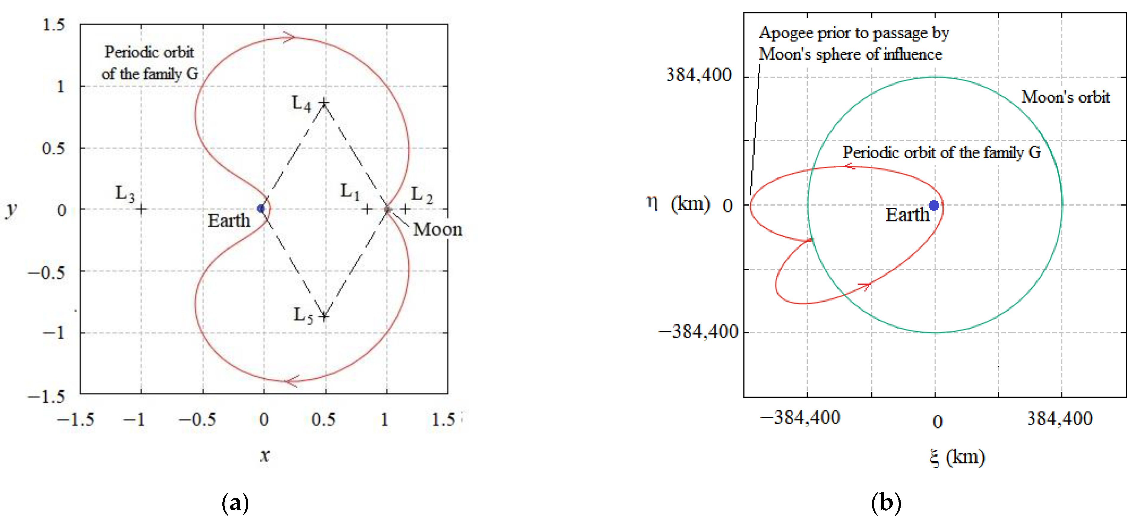
2. Circular Restricted Three-Body Problem (CR3BP) and Family G of the Periodic Orbits around the Lagrangian Point L₁

The Circular Restricted Three-body Problem (CR3BP) is well known in the literature [3,33]. It describes the motion of a particle with mass $m$ under the action of the gravitational fields of two other so-called primary masses, $m_{P_1}$ and $m_{P_2}$. The particle’s mass is negligible, and it does not affect the motion of the primary masses whose orbits are circular and coplanar around their common center of mass, both with the same angular velocity; therefore, they also maintain a constant distance between them. These properties allow the introduction of an orthogonal reference frame $\left(x, y, z\right)$ called a synodic frame whose origin is at the common center of mass of the primary masses and in which these bodies are fixed over the x-axis with coordinates $\left(x_1, y_1, z_1\right)=\left(-{\mu }_{P_2}, 0, 0\right)$ and $\left(x_2, y_2, z_2\right)=\left({\mu }_{P_1}, 0, 0\right)$, i.e., x- and y- axes rotate with the same angular velocity as the primary masses relative to an inertial frame (also fixed at the common center of mass). It is useful to consider the normalization of this frame, such as the sum of the primary gravitational mass parameters being equal to 1, that is, $\mu ={\mu }_{P_1}+{\mu }_{P_2}=1$, with ${\mu }_{P_1}=m_{P_1}/\left(m_{P_1}+m_{P_2}\right)$ and ${\mu }_{P_2}=m_{P_2}/\left(m_{P_1}+m_{P_2}\right)$ and the distance between the primary masses is also equal to 1 (unit of measurement). In this way, the mean motion and the orbital period of the primaries are equal to 1 and 2$\pi$, respectively.

For the CR3BP with an Earth–Moon mass ratio, $m_{P_1}=m_{Earth}=5.9724\times {10}^{24}$ kg and $m_{P_2}=m_{Moon}=7.3460\times {10}^{22}$ kg. Thus, ${\mu }_{P_1}=0.987849536$ and ${\mu }_{P_2}=0.012150463$. The distance between $m_{P_1}$ and $m_{P_2}$ corresponds to the average distance between the Earth and the Moon, 384,400 km, and their orbital period is 27.32166 days.

The equations of motion of the CR3BP have five special solutions that define the so-called Lagrangian equilibrium points. Three of them, L₁, L₂, and L₃, are aligned with the primary masses, while the other two, L₄ and L₅, form two equilateral triangles with the primaries. These points can be seen in Figure 1a.

Broucke [3] numerically examined several families of periodic orbits considering the CR3BP with the Earth–Moon mass ratio. Family G (“G” in capital letter) of retrograde periodic orbits around L₁ is one of them. Family G corresponds to Class “c” of orbits around L₁ in Stromgren’s problem with an equal mass ratio [34]; however, the orbits of Class “c” have different evolution, and their symmetry is with respect to both x- and y- axes, while the orbits of family G have symmetry only with respect to the x-axis.

The periodic orbits of family G can be found by numerical integration considering the following initial condition for a particle, at $t_0=0,$ in the synodic frame,

$$\left(x_0,y_0,z_0,{\dot{x}}_0,{\dot{y}}_0,{\dot{z}}_0,t_0\right)=\left(x_0,0, 0, 0,{\dot{y}}_0,0, 0\right).$$

(1)

For instance, by taking $x_0=0.049999990$ and ${\dot{y}}_0$ = 5.458017660, the periodic orbit shown in Figure 1 is found. In general, periodic orbits of family G can be obtained for $0.012149617 \le x_0 \le 0.813471672$ and $-1.950882153 \le {\dot{y}}_0 \le 601.045380978$ [3]. Periodic orbits such as that shown in Figure 1 for (a) synodic (x, y, z) and (b) geocentric (ξ, η, ζ) frames pass remarkably close to the Earth’s surface and, after 14 to 15 days, they pass a few dozens of kilometers away from the Moon’s surface, so they form a round-trip link between them. In addition, the periodic orbits of family G are sensitive to minor perturbations in their velocities. These features can be explored to generate interplanetary trajectories, as described in the next section.

According to Equation (1), for any periodic orbit of family G, at $t_0=0,$ the Earth, spacecraft, and Moon must be aligned in this order, i.e., in inferior conjunction. Therefore, considering the spacecraft in a circular LEO, the spacecraft and the Moon have parallel velocities. In practical terms, this alignment is a weak constraint, because any spacecraft orbiting the Earth in the same plane as the Moon’s orbit will achieve this alignment every orbital period, plus a small period of time to compensate for the Moon’s displacement. For example, for circular LEOs with altitudes of 200, 400, 700, and 1000 km, the alignments are obtained at approximately 88.38 min + 11.88 s, 96.57 min + 14.22 s, 98.66 min + 14.84 s, and 105 min + 16.81 s, respectively.

3. Definition of the Trajectories G

This section describes the trajectories derived from the periodic orbits of family G in more detail, hereinafter referred to as trajectories G, or simply TGs. It covers two approaches to define them, as well as other properties.

3.1. The CR3BP and a First Approach for the TGs

Considering a spacecraft in circular parking orbits (LEOs) with altitudes between 200 km and 1000 km, the two-dimensional CR3BP, Earth, spacecraft, and Moon alignment at $t_0=0$, and the performance of small variations in the speeds (same direction of motion) of the periodic orbits of the family G [3], a first approach for the insertion speeds ($V_{SC}$) of spacecraft into trajectories G is obtained. These TGs are tangential to the LEOs and capable of passing between L₁ and the Moon’s surface, colliding with the Moon, or escaping from the Earth–Moon system. The values of V_SC are given in m/s by

$$V_{SC}=-8.571050\times {10}^{-4}{h}_0+\mathrm{11,105.303}+{\vartheta }_{3B},$$

(2)

where $h_0$ is the altitude of the circular LEOs $\left(0 \le h_0\le {10}^6 \mathrm{m}\right)$, and ${\vartheta }_{3B}$ values define the point between L₁ and the Moon’s surface on the x-axis of the synodic frame the trajectories pass through, and whether they are collision or escape trajectories. For ${\vartheta }_{3B}=-0.976 \mathrm{m}/\mathrm{s}$, the trajectory crosses the x-axis at point L₁; for $0\le {\vartheta }_{3B}\le 0.322 m/s$, collisions trajectories are found; and for ${\vartheta }_{3B}>0.322 \mathrm{m}/\mathrm{s}$, escape trajectories from the Earth–Moon system arise. The $\Delta V$ to generate trajectories G ($|\Delta V_{TG}|)$ as a function of $h_0$, i.e., from circular LEOs, can be seen in Section 3.2.2. However, Equation (2) can be used to obtain the $\Delta V_{TG}$ for any geocentric orbit, for example, from the apogee of an ellipse.

To obtain Equation (2), numerical simulations were conducted. In these, small increments in the spacecraft velocities were added to insert them into different kinds of TGs. The characteristic $V_{SC}$ for each kind of TG was then registered, and linear regression with the points found gave form to Equation (2).

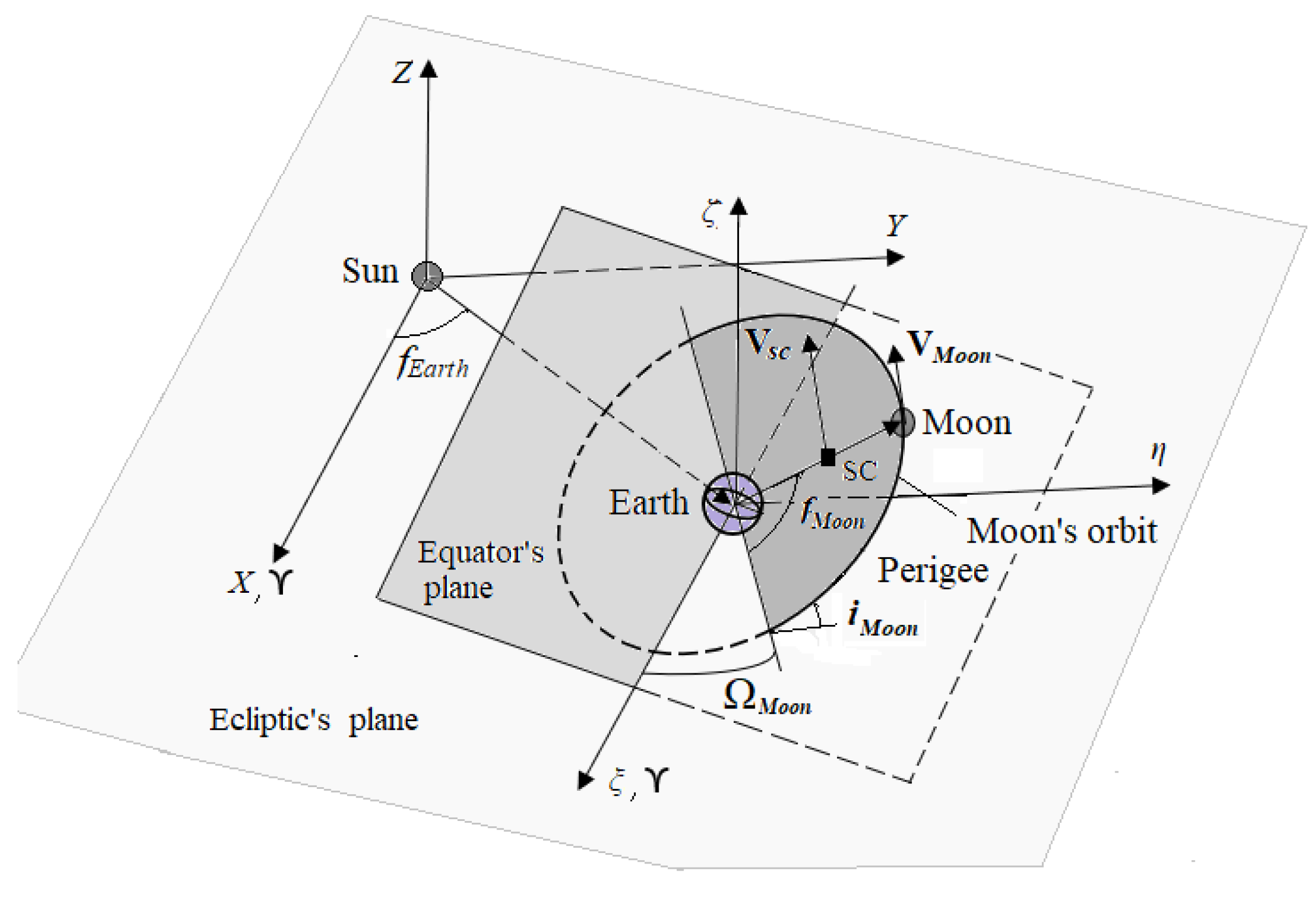
3.2. The Three-Dimensional Restricted Full Four-Body Problem Sun-Earth-Moon-Particle (FR4BP)

To better understand the properties of the trajectories G and possible applications, the three-dimensional Restricted Full Four-body Sun-Earth-Moon-spacecraft Problem (FR4BP) is considered. In this dynamical system, indexes 1 through 4 are associated with the Sun, Earth, Moon and a spacecraft with negligible mass ($m_4$), respectively. The same normalization adopted for the CR3BP is also adopted for the FR4BP. Thus, ${\mu }_1=m_1/\left(m_2+m_3\right)$, ${\mu }_2=m_2/\left(m_2+m_3\right)$, ${\mu }_3=m_3/\left(m_2+m_3\right)$, and ${\mu }_4=m_4/\left(m_2+m_3\right)$ are the gravitational mass parameters of the Sun, the Earth, the Moon and the spacecraft, respectively; and now ${\mu }_2+{\mu }_3=1$. The normalization is completed by adopting the average distance between the Earth and the Moon (384,400 km) as a unit of measurement. These four bodies move in three-dimensional space under mutual attraction, and the equation of motion of the i-th body in a coordinate frame (X, Y, Z) with the origin at any point in space is

$${\ddot{\mathit{R}}}_i={{\displaystyle \sum }}_{\begin{array}{c}j=1\\ j \ne i\end{array}}^4\frac{{\mu }_j}{R_{ji}^3}\left({\mathit{R}}_j-{\mathit{R}}_i\right),$$

(3)

where ${\mathit{R}}_i=\left(X_i, Y_i, Z_i\right)$ is the position of the i-th body, $R_{ij}=\left|{\mathit{R}}_j - {\mathit{R}}_i\right|$ $={\left[{\left(X_j - X_i\right)}^2+{\left(Y_j - Y_i\right)}^2+{\left(Z_j - Z_i\right)}^2\right]}^{1/2}$, with j ≠ i, is the distance between the i- and the j-th bodies and ${\ddot{\mathit{R}}}_i$ is the acceleration of the i-th body. Equation (3) is a set of 12 s-order differential equations and expresses the fact that the acceleration of a given body is the result of the sum of the forces exercised by the other three bodies.

3.2.1. The Three-Dimensional Restricted Bicircular Four-body Problem (BCR4BP) and a Second Approach for the TGs

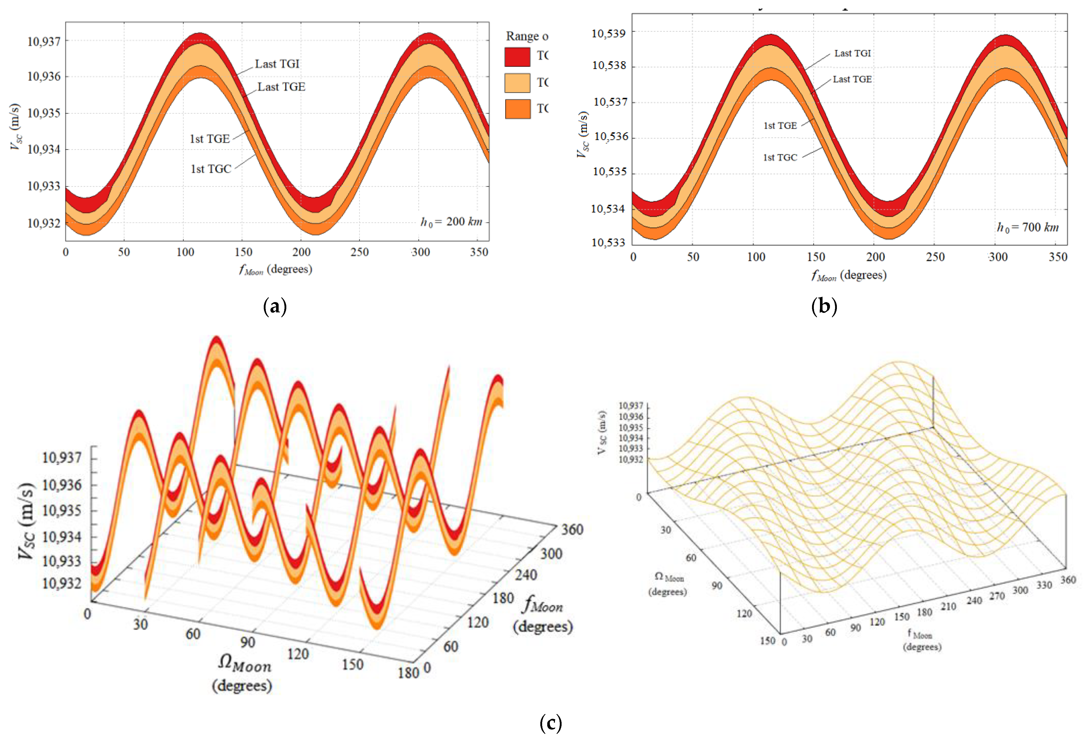
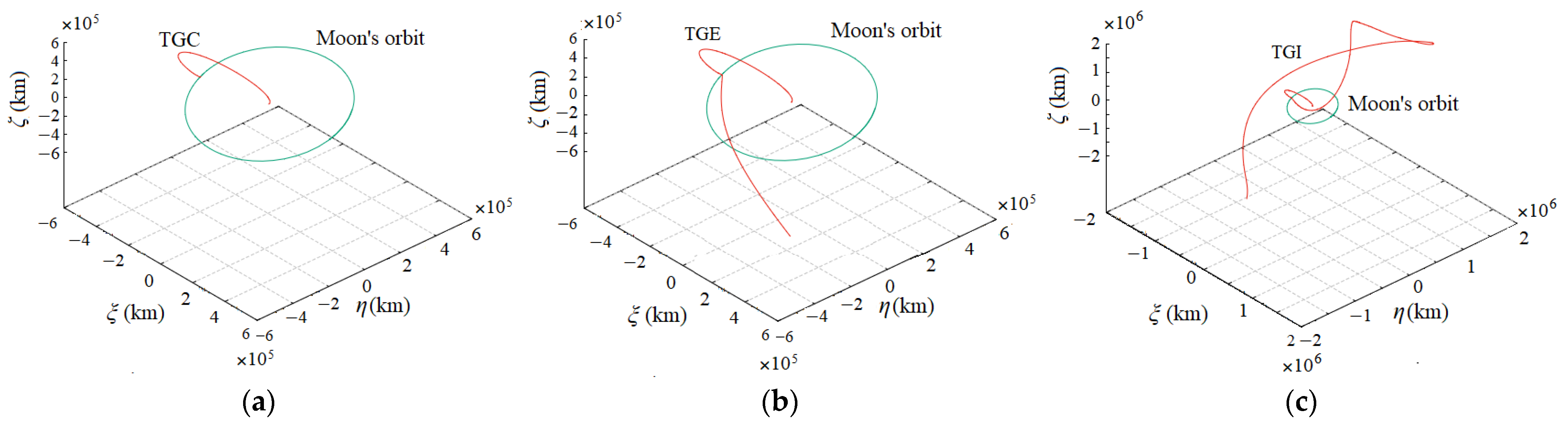
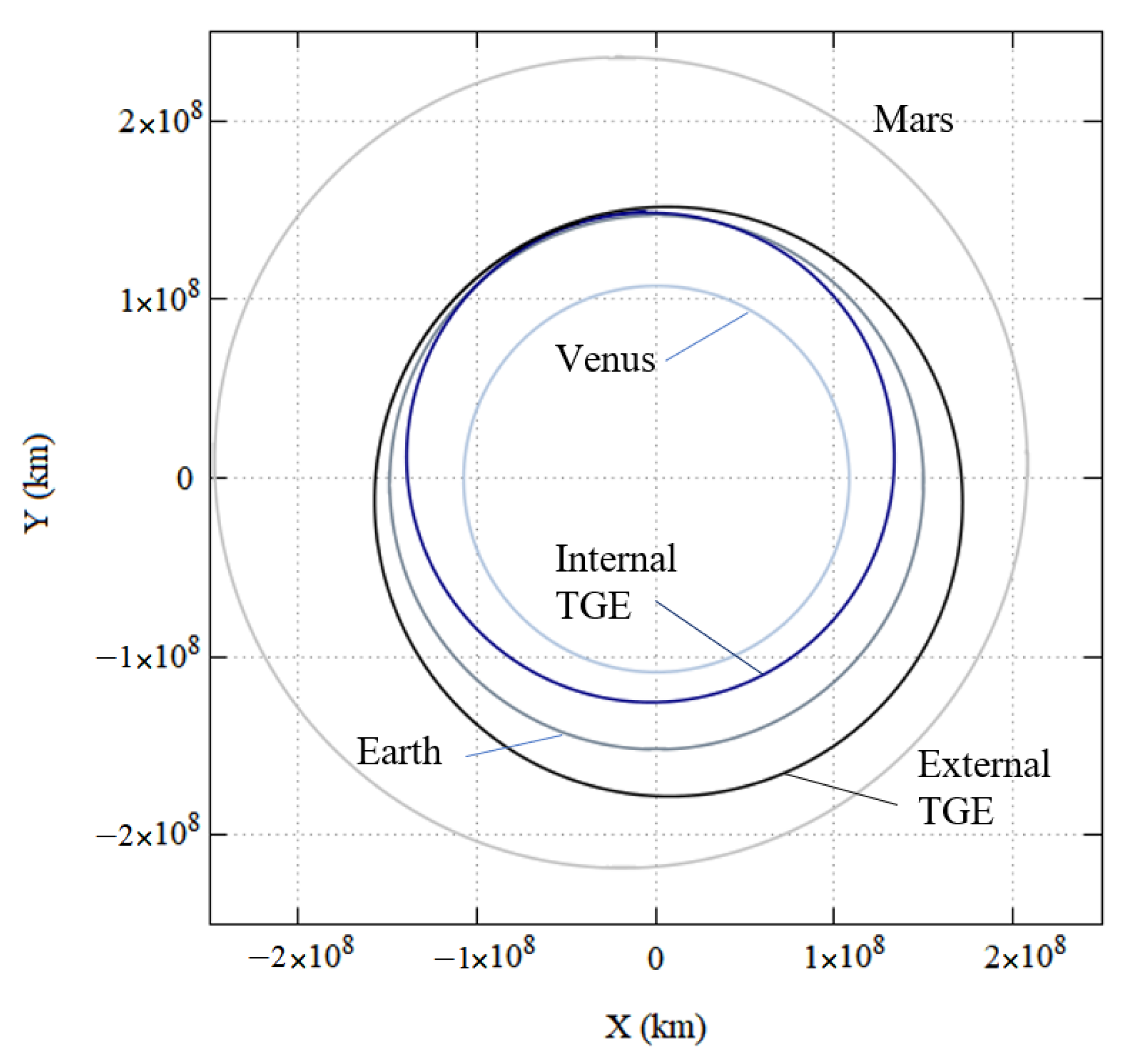
The introduction of the Sun into the dynamical system makes the definition of $V_{SC}$ more complex due to the relative positioning between the four bodies. To describe this, a particular arrangement of the Four-body Problem, in which the Earth’s orbit around the Sun and the Moon’s orbit around the Earth is circular (BCR4BP), is adopted as a second approach. The semimajor axes (a), eccentricities (e), inclinations (i), and true anomalies (f) considered are: $a_{Earth}$ = 149,597,870.8 km (1 au), $a_{Moon}$ = 384,400 km, $e_{Earth}$ = $e_{Moon}$ = 0, $i_{Earth}$ = 0°, $i_{Moon}$ = 28.56°, and, naturally, $0 \le f_{Earth}<360°$ and $0 \le f_{Moon}<360°$. The longitude of the ascending node ($\Omega$) is undefined for circular orbits with i = 0°, and the argument of periapsis (ω) is undefined for circular orbits of any inclination, so ${\Omega }_{Earth}={\omega }_{Earth}={\omega }_{Moon}=0°$ and $0 \le {\Omega }_{Moon}<360°$. However, these values are taken only to provide a step-by-step method to determine $V_{SC}$ for the trajectories G in this second approach. The numerical method that will be presented in the next section allows for adjusting $V_{SC}$ to the current and future values of the orbital elements of the Earth’s and the Moon’s orbits as well as their instantaneous variations.

Figure 2 presents a general illustration of the relative positioning between the Sun, Earth, a spacecraft ($SC$), and the Moon at launch time ($t_0$) for the BCR4BP, precisely when the spacecraft is in a circular LEO and acquires the insertion speed ($V_{SC}$) into a trajectory derived from a periodic orbit of family G relative to the geocentric frame (ξ, η, ζ). $V_{SC}$ is parallel to the Moon’s velocity. Note also that the Earth, spacecraft, and Moon are aligned in this order, as described in Section 2, but the Sun alignment is not necessary.

Considering the same procedure described in Section 3.1 (for the CR3BP), but now for the BCR4BP, and varying f_Moon and ${\Omega }_{Moon}$, a second approach for the insertion speeds (V_SC) into TGs can also be found. For the BCR4BP, V_SC depends on the h₀, f_Moon, and ${\Omega }_{Moon}$. The dependence of V_SC with h₀ remains linear as in the CR3BP, while ${\Omega }_{Moon}$ and f_Moon are approximately sinusoidal with a period of 14.746107 days (3.392 rad), in agreement with the circular dynamics of the system. As a result of this procedure for the BCR4BP, V_SC (m/s) can be obtained by

$$V_{SC}=-8.481880\times {10}^{-4}{s}^{-1}{h}_0+\mathrm{11,103.421}+{\vartheta }_{4B}+Asin\left[B\left({\Omega }_{Moon}+f_{Moon}\right)+C\right],$$

(4)

where ${\vartheta }_{4B}$ varies continuously, such that:

• For $0\le {\vartheta }_{4B}\le 0.312\pm 0.008 \mathrm{m}/\mathrm{s}$, TGs that collide with the Moon are found (they are called “trajectories G of collision”, TGCs).
• For $0.312\pm 0.008<{\vartheta }_{4B}\le 0.667\pm 0.021 \mathrm{m}/\mathrm{s}$, TGs that have encounters with the Moon, gain energy, and escape from the Earth–Moon system are found (they are called “trajectories G of direct escape”, TGEs).
• For $0.667\pm 0.021<{\vartheta }_{4B}\le 1.023\pm 0.030 \mathrm{m}/\mathrm{s}$, TGs that approach and have an encounter with the Moon, but do not gain enough energy to escape from the Earth–Moon system, are found (they are called “trajectories G of inversion”, TGIs).

The values of A, B, and C have small variations according to the type of trajectory G obtained, i.e., according to ${\vartheta }_{4B}$, and they are determined numerically, being $A=2.227 \pm 0.074 \mathrm{m}/\mathrm{s}$, $B=2\pi /3.392=1.852442\pm 0.001036$, and $C=121.75514\pm 1.412805$. For example, in Figure 3a, for which h₀ = 200 km, ${\Omega }_{Moon}$ = f_Earth = 0° at t₀ = 0, and for $0\le f_{Moon}\le 360°$, the curve for the first TGC as a function of f_Moon is

$$V_{SC}=\mathrm{10,933.784}+2.158sin\left(1.852755f_{Moon}-2.149686\right),$$

(5)

for the first TGE,

$$V_{SC}=\mathrm{10,934.088}+2.169sin\left(1.853478f_{Moon}-2.144921\right),$$

(6)

for the last TGE,

$$V_{SC}=\mathrm{10,934.600}+2.301sin\left(1.851406f_{Moon}-2.100370\right)$$

(7)

and for the last TGI,

$$V_{SC}=\mathrm{10,934.902}+2.262sin\left(1.853101f_{Moon}-2.118499\right).$$

(8)

Equations (5)–(8) were obtained by the least-squares method, using the same procedure described in Section 3.1 to obtain the simulation data. The standard deviation for Equations (5)–(8) are 0.028 m/s, 0.028 m/s, 0.033 m/s, and 0.033 m/s, respectively.

The dependence on h₀ and f_Moon are highlighted in Figure 3a,b, in which h₀ is equal 200 km and 700 km, respectively, with the curves obtained for ${\Omega }_{Moon}$= 0° at t₀ = 0. The dependence of V_SC on f_Moon and ${\Omega }_{Moon}$ for h₀ = 200 km is shown in Figure 3c.

A TGC, TGE, and TGI obtained for a particular positioning defined by ${\Omega }_{Moon}$ = f_Moon = 0, at t₀ = 0, can be seen in Figure 4 (remember that ${\Omega }_{Earth}$ = ω_Earth = 0). For these values, the Sun, Earth, spacecraft, and Moon are aligned in this order over the X-axis of the coordinate frame with an origin at the Sun’s center of mass. Considering the scale used in Figure 4, the three TGs are overlapping in the initial phase, i.e., during the flight between the Earth and the Moon, with subtle differences, as will be described in the next subsection.

In Section 4, the actual ephemerides of the Earth’s and the Moon’s orbits will be considered for application in missions to NEAs. In this case, the curves for TGCs, TGEs, and TGIs lose their sinusoidal profile and numerical analysis is required.

3.2.2. Some Features of the TGs in the BCR4BP

As stated previously, TGs are generated by applying $\Delta V_{TG}$ to spacecraft in circular LEOs whose altitudes vary between 200 km and 1000 km. Therefore, $|\Delta V_{TG}|=V_{SC}-\sqrt{G{M}_{Earth}/\left(R_{Earth}+h_0\right)}$, where V_SC is given by Equation (4), $R_{Earth}=6371 \mathrm{km}$ is Earth’s average radius, and the square root provides the LEOs speeds as a function of the altitude h₀ (Figure 5b). Figure 3, in turn, shows the dependence of V_SC with f_Moon and ${\Omega }_{Moon}$, and it is possible to note that for fixed values of h₀ and f_Moon, the difference between the speeds of the first TGC and last TGI is in the order of 1.050 m/s. On the other hand, the sinusoidal dependence of V_SC with f_Moon for any h₀ and ${\Omega }_{Moon}$ shows that the difference between the minimum V_SC to generate the TGC and the maximum V_SC to generate the last TGI is in the order of 4.6 m/s (Figure 5a). Consequently, the minimum and maximum $|\Delta V_{TG}|$ to generate TG will also vary by 4.6 m/s as shown in Figure 5c.

The TGs reach apogees of approximately 540,000 km (first TGC) and 550,000 km (last TGI) prior to their passage through the lunar sphere of influence between 8 and 9 days after the launch. The apogees are positioned approximately on the ξ-axis of the geocentric frame as shown in Figure 1b. At the apogees, the speeds of TGs vary between 155 m/s (first TGC) and 149 m/s (last TGI). Therefore, the regions near these apogees could be employed for correction maneuver areas.

The TGs reach their periselenes between 14 and 15 days after the launch, and all of them have their specific orbital energy relative to the Earth (ε₂₄—following the indices adopted in Section 3.1) increased during the passage through the lunar sphere of influence. However, the same does not occur for their specific orbital energy relative to the Sun (ε₁₄).

To understand the increase in ε₂₄, first we consider the angle between the directions defined by a given position vector relative to the Moon at periselene and the straight line joining the centers of the Earth and the Moon (Ψ). According to Broucke [23], the change in the specific orbital energy of a spacecraft’s trajectory relative to the Earth (first body) after a swing-by with the Moon (second body), in three-body dynamics, (Δε₂₄) is $\Delta {\epsilon }_{24}={\epsilon }_{24}\left(t_2\right)-{\epsilon }_{24}\left(t_1\right)\propto -sin\left(\mathsf{\Psi }\right)$, where ε₂₄(t₁) and ε₂₄(t₂) are the specific orbital energies of the trajectory relative to the Earth when it penetrates and leaves the lunar sphere of influence, respectively. Therefore, the largest Δε₂₄ is obtained for Ψ = 270°. As an example, Figure 6 presents the relations between $\Delta {\epsilon }_{24}$ × $\mathsf{\Psi }$, $\Delta {\epsilon }_{24}$ × V_SC and periselene radius × $\mathsf{\Psi }$ for TGEs and TGIs generated for for h₀ = 200 km, ${\Omega }_{Moon}$ = f_Moon = f_Earth = 0 at t₀ = 0 and the BCR4BP dynamics. It is possible to verify in Figure 6a that all TGEs and TGIs have Δε₂₄ > 0, as expected, and that the largest value of Δε₂₄ corresponds to Ψ = 266° (≈ 270°)—the TGCs have been excluded from this analysis. It is also possible to verify, in Figure 6b, that the largest value of Δε₂₄ occurs for the smallest value of V_SC capable of generating a TGE; and in Figure 6c, the smallest periselene corresponds to Ψ = 266° (≈270°) and, in comparison with Figure 6a, consequently, it corresponds to the largest value of Δε₂₄. These results show that the increase in the specific orbital energy relative to the Earth, ε₂₄, in the CR4BP dynamics follows, with a slight difference, that predicted by three-body dynamics.

Now, in the BCR4BP, the largest changes in the specific orbital energy of the TGs relative to the Sun (Δε₁₄) can occur for more than one value of V_SC and Ψ as shown in Figure 7. Δε₁₄ = ε₁₂ − ε₁₄(300), where ε₁₂ is the Earth’s specific orbital energy (= −443.298 MJ/kg) taken as a reference, and ε₁₄(300) is the TG’s specific orbital energy at t = 300 days, both relative to the Sun. The interval of 300 days was chosen because, from then on, the osculating orbital elements of trajectories G undergo only small variations in general. Still, in the context of the BCR4BP, Δε₁₄ < 0 corresponds to TGEs with perihelia between Earth’s and Venus’ orbits and aphelia of approximately 1 au; Δε₁₄ ≈ 0 corresponds to TGIs (therefore, co-orbitals to Earth’s orbit relative to the Sun), and Δε₁₄ > 0 are TGEs with aphelia between the Earth’s and Mars’ orbits and perihelia of approximately 1 au. In the example of Figure 7, the smallest Δε₁₄ (Δε₁₄ = −20.46 MJ/kg) occurs for Ψ ≈ 266° and the smallest V_SC value (V_SC = 10,932.280 m/s—the smallest V_SC that generates a TGE for h₀ = 200 km, ${\Omega }_{Moon}$ = f_Moon = 0 at t₀ = 0); and the largest Δε₁₄ (Δε₁₄ = 23.49 MJ/kg) is obtained for Ψ ≈ 247° and V_SC = 10,932.467 m/s. The first one has the smallest perihelion (0.84 au), near the orbit of Venus, and the largest internal reach, while the second one has the largest aphelion, near the orbit of Mars (1.156 au), and the largest external reach.

Thus, Δε₁₄ can generate internal TGEs (with perihelia between Venus’ and Earth’s orbits and aphelia at 1 au) and external TGEs (with aphelia between Earth’s and Mars’ orbits and perihelia at 1 au), and the type of TGE depends on $\mathsf{\Psi }$ and V_SC. The dependence on V_SC consequently leads to dependence on f_Moon and ${\Omega }_{Moon}$ as seen in Equation (4). Figure 8a shows the distribution of perihelia and aphelia for internal TGEs and Figure 8b shows the distribution for external TGEs, for both ${\Omega }_{Moon}$ = 0° at t₀ = 0. For this initial condition, the internal TGEs closest to Venus have perihelia and aphelia in the order of 125 × 10⁶ km and 150 × 10⁶ km, respectively; while the TGEs farthest from Earth toward Mars have perihelia and aphelia radii in the order of 150 × 10⁶ km and 182 × 10⁶ km, respectively. These distributions are always similar for any value of ${\Omega }_{Moon}$ and h₀. That is, the smallest perihelion and the largest aphelion found for the TGEs are in the order of 125 × 10⁶ km and 182 × 10⁶ km, respectively.

Figure 9 presents the TGEs with the smallest perihelion and the largest aphelion. For the first, h₀ = 200 km, V_SC = 10,936.100 m/s, f_Earth = 92.2440048°, ${\Omega }_{Moon}$ = 0°, and f_Moon = 30° at t₀ = 0, the perihelion is 125,305,866.0 km (0.8376 au), achieved at 493.63 days after the launch, and its aphelion is 149,986,525 km (1.0026 au), achieved at 20.48 days after the launch. For the second, h₀ = 200 km, V_SC = 10,936.093 m/s, f_Earth = 106.83059°, ${\Omega }_{Moon}$ = 0°, f_Moon = 225° at t₀ = 0. The perihelion is 150,998,982.0 km (1.00937 au) achieved at 20.05 days after the launch, and its aphelion is 180,340,233.0 km (1.2055 au) achieved at 224.43 days after the launch.

The longitude of the ascending node and the argument of periapsis of the TGs depend on the launch date (because of the relative positioning between the Sun, Earth, and Moon), but their inclinations are always less than 2° with respect to the ecliptic in general.

Returning to Figure 5 and comparing the $|\Delta V_{TG}|$ and $\left|\Delta V_{esc}\right|$, i.e., the speed changes required to generate TGs and conventional escape trajectories, $\left|\Delta V_{TG}\right|$ is always smaller than $|\Delta V_{esc}|$. $\left|\Delta V_{TG}\right|$ is 2.5% smaller than $\left|\Delta V_{esc}\right|$ for h₀ = 200 km, and 4.6% smaller for h₀ = 1000 km. On the other hand, the heliocentric trajectory generated with a conventional $|\Delta V_{esc}|$ will have perihelia in the order of 145 × 10⁶ km and aphelia in the order of 151.5 × 10⁶ km, much smaller than those achieved by TGEs. In the next section, some examples for transferring spacecraft to NEAs will be exposed and the $\left|\Delta V_{TG}\right|$ required for these missions is approximately 5% smaller than the $|\Delta V$| required for interplanetary trajectories obtained by Lambert’s Method.

4. Applications

Studies and results on transfers to the NEAs 3361 Orpheus (Apollo class), 99,942 Apophis (Aten class), and 65803 Didymos (Apollo class) through TGEs are presented in this section. However, a general introduction to the planning of these transfers is required first. In this section, all numerical simulations consider the Restricted Full Four-body Problem (FR4BP) describes in Section 3.2 as a dynamical system.

4.1. Limits of the TGs

In Figure 8, it is possible to identify 124,814,014.0 km and 181,272,593.0 km as the lower and upper limits achieved by TGEs in the first analysis, respectively. From a geometrical standpoint, these values can be interpreted as the radii of two reference circumferences in the plane of the ecliptic (since the inclination of the TGEs is small), one internal with radius R_i = 124,814,014.0 km and one external with radius R_e = 181,272,593.0 km. The space between them defines the primary interception region of NEAs by TGEs. Figure 10 presents an illustration of this region, and, in broad terms, the analysis of a transfer starts when an asteroid penetrates it. On the other hand, considering the features of the NEAs orbits, those belonging to the Apollo class can cross the two reference circumferences or only the external one, some NEAs belonging to the Aten class can be located completely inside the primary region, while some orbits of Amor class can only cross the external reference circumference and some orbits of Atira class can only cross the internal reference circumference.

Due to the small inclinations relative to the ecliptic of the TGEs, the interceptions of the NEAs can only occur in a range near their nodes and if they are within the primary interception region. The lower the inclination of the NEA, the greater the possibility of interception.

4.2. Parameters for Planning Transfers to NEAs by TGEs

The step-by-step sequence for planning a transfer is as follows:

• Step 1: Choose an NEA and an interval of interest for planning a mission. Once this choice is made, data on the orbits of the NEA, Earth, and Moon (orbital elements or vectors state) must be obtained through an orbit propagator or, for example, from JPL’s Horizons platform for this interval [35].
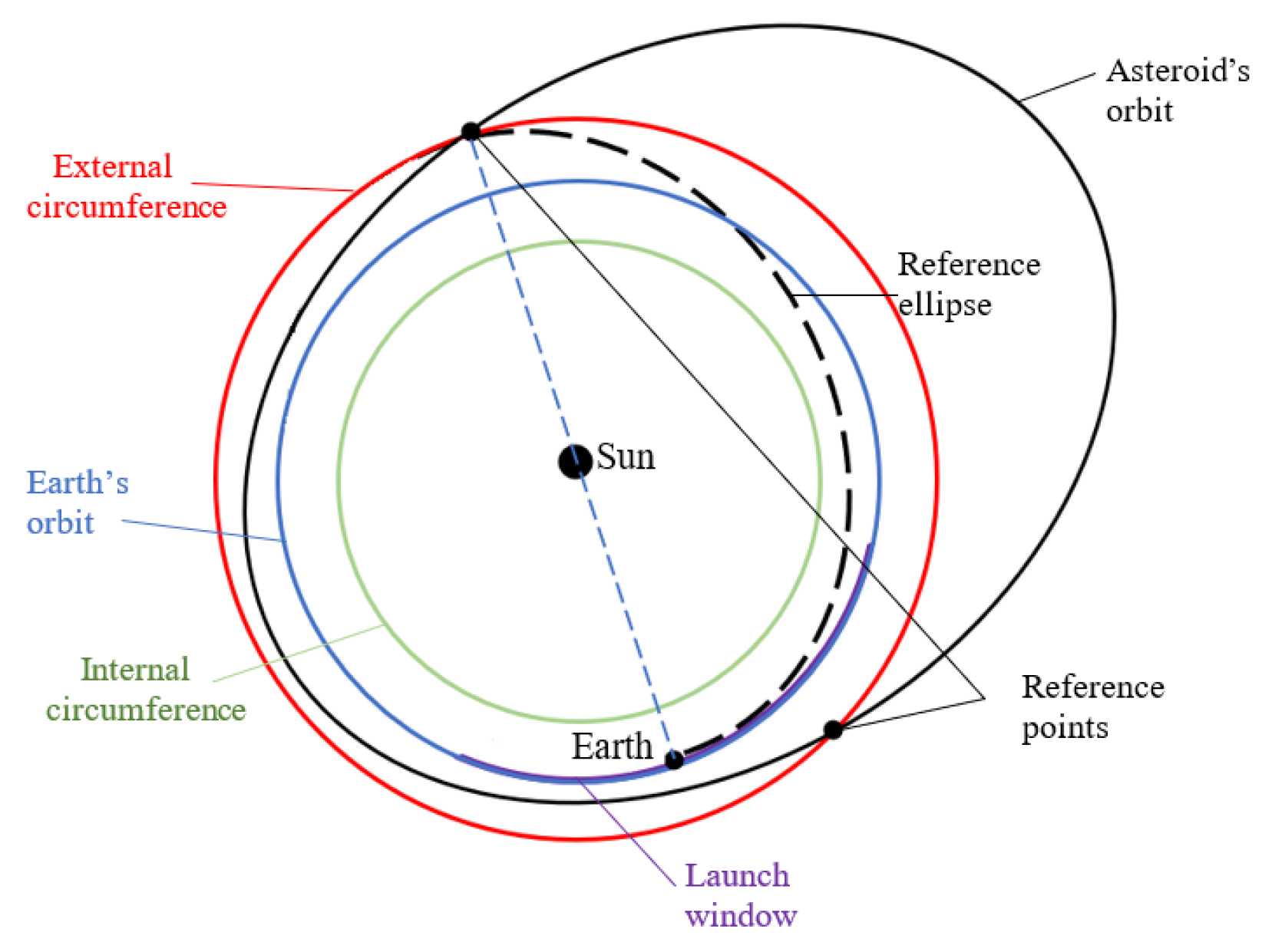
• Step 2: Considering the data obtained for the NEA’s orbit in step 1, it is necessary to determine if it passes through the primary intercept region, the dates of entry and exit from this region, and the respective position (relative to the Sun), and if its nodes are also in this region. If the nodes are in this region, there is a great probability of finding a TGE able to intercept the chosen NEA. Otherwise, this probability becomes smaller, so even an interception continues to be possible.
• Step 3. Firstly, considering the case in which the nodes are in the primary intercept region, from the straight lines segments that join these points to the Earth’s orbits through the Sun, it is possible to define the semimajor axes of two references ellipses and their orbital periods. Subtracting half of these orbital periods and adding 20 days (time needed for a TGE to reach the Earth’s sphere of influence) from the dates corresponding to the passages of the NEA through its ascending or descending nodes, two new dates are found, and they will be the starting point for definition (or study) of the launch windows. Figure 10 shows a reference ellipse considering that the points in which the NEA’s orbit entries and exits the intercept region coincide with its nodes. In this example, the semimajor axis is (149,597,870.7 km + 181,272,593.0 km)/2 = 165,435,231.9 km, and half of the orbital period is 212.4 days, plus 20 days, totaling 232.4 days. Then, the date found can be adopted as the beginning of the launch window, since the Earth is within the launch window interval. An interval of three lunar cycles, approximately 82 days, is generally enough to obtain some TGEs able to carry out an Earth–NEA transfer.
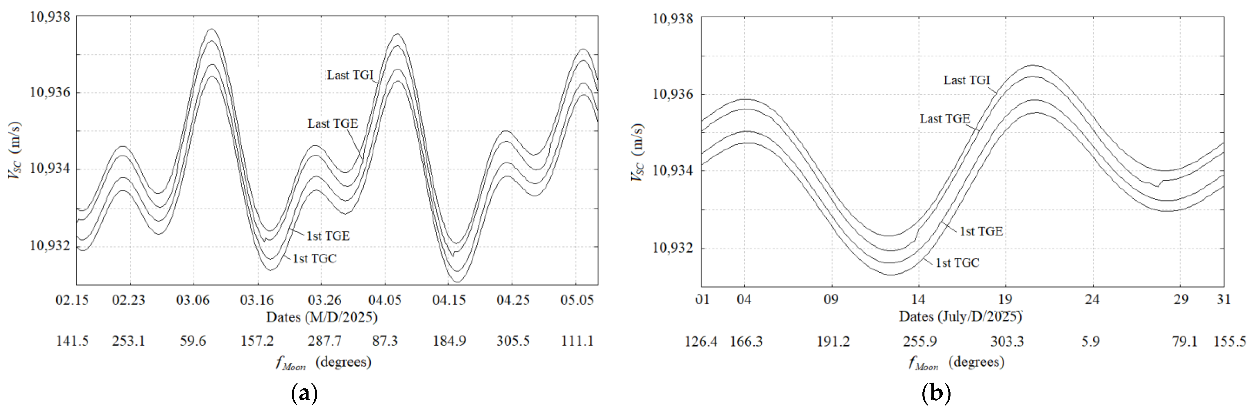
• Step 4. From the new dates found in step 3, intervals containing these dates are defined, and they will be considered the first choice for the launch window. Following this, a set of simulations are conducted to find TGEs able to intercept the NEA chosen. First, the curves V_SC × f_Moon for these intervals are found; then, from the V_SC that defines the TGEs for these intervals, trajectories are propagated to obtain encounters with the NEA.
• Step 5. Analyses of the results.

4.3. Analysis for the Transfers to the 3361 Orpheus (Apollo Class), 99942 Apophis (Aten Class), and 65803 Didymos (Amor Class)

Table 1. Properties of the NEAs 3361 Orpheus, 99942 Apophis, and 65803 Didymos (JD 2459126.5 4 October 2020).

Property	Orpheus	Apophis	Didymos
Class	Apollo	Aten	Apollo
Mass *	4.66 × 1010 kg	2.70 × 1010 kg	5.27 × 1010 kg
Dimension	AR = 150 m, L = 300 m	370 m × 450 m × 170 m	AR = 390 m
Absolute Magnitude (H)	19.03	19.70	18.07
Semimajor axis	180,962,886.3 km	137,994,462.3 km	246,025,217.4 km
Eccentricity	0.322752	0.191195	0.383638
Inclination	2.68°	3.33°	3.41°
Longitude of ascending node	189.53°	204.45°	73.21°
Argument of perihelion	301.66°	126.40°	319.30°
Orbital period	1.33 Years	0.89 Years	2.11 Years

* Estimated for calculation, AR = average radius, L = length. Source: [36].

presents some features of the NEAs 3361 Orpheus, 99942 Apophis, and 65803 Didymos and their orbits. They are considered in transfer simulations from TGEs.

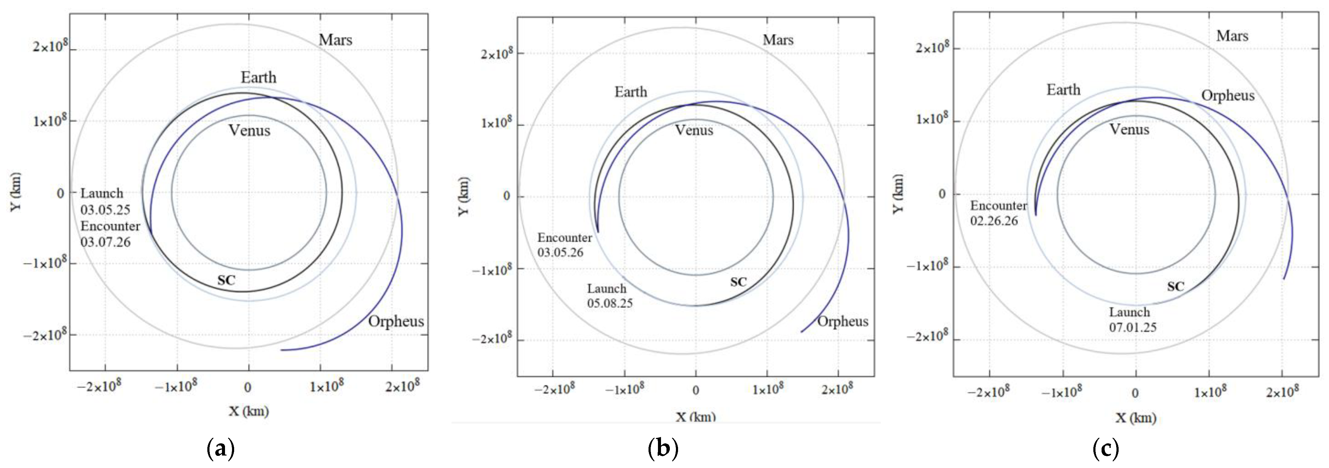
4.3.1. Transfer to the 3361 Orpheus

Considering the 2025–2026 biennium, for example, and applying the steps of the previous subsection, the dates in which the Orpheus’s orbit enters and exits the primary intercept region are 4 October 2025 and 16 April 2026, respectively. Three transfers to this NEA via TGEs for two different launch windows can be planned. Subtracting half of the orbital period of the reference ellipse (233.1 days) from these dates, the launch window will be between 15 February and 1 July 2025.

Table 2. Properties of the Earth-NEA 3361 Orpheus transfers.

Property	First Transfer	Second Transfer	Third Transfer
Launch window M/D/Y	02/15/25–05/08/25	02/15/25–05/08/25	07/01/25–07/30/25
Launch date M/D/Y	12 h-03/05/25	0 h-05/08/25	0 h-07/01/2025
Circular parking LEO altitude (km)	200
VSC (m/s)	10,935.561	10,935.550	10,934.480
|ΔVTGE | (m/s)	3153.635	3153.362	3152.553
|ΔV| at aphelion (m/s)	48	18	12
|ΔVLaunch| (reference) Lambert’s Method * (m/s)	3330
Launch C3 relative to the Earth (106 m2/s2)	−1.530	−1.531	−1.55
Impact date, M/D/Y	03/07/2026	03/05/2026	02/26/2026
Time of transfer (days)	367.89	301.18	230
Distance from Earth at impact (km)	376,576,144.4 km	325,347,488.6 km	89,997,492.0 km
Arrival Impact Angles (degrees)	16.80	10.73	8.89
Relative velocity at impact (m/s)	9886.548	6383.805	6082.983

* Without middle-way correction maneuvers.

presents the main information about each transfer between 2025 and 2026. In all three transfers, correction maneuvers are required approximately 25 days after the launch, at the aphelion of the TGEs, to cause impact. For the first launch (on 5 March 2025), a distance of 1.5 × 10⁶ km between the spacecraft and the NEA at the closest point approach (CPA) must be overcome. A |ΔV| of approximately 48 m/s applied at the aphelion is enough to reduce this distance to zero. For the second launch (on 8 May 2025), the distance to be overcome is approximately 1.3 × 10⁶ km, and a |ΔV| of approximately 18 m/s applied at the aphelion is also enough. For the third launch (on 1 July 2025), the distance between them is 404,000 km at the CPA, and it is overcome with a |ΔV| of approximately 12 m/s applied at the aphelion. The ΔVs for correction maneuvers are calculated to increase or decrease the energy of the TGE (at this point, a heliocentric ellipse) from the vis-viva equation to ensure the NEA-spacecraft distance is null at the encounter. They are applied to the direction of the spacecraft’s motion when it is at the aphelion. Other parameters of these missions, such as |ΔV| launch, the day of arrival/impact, the relative speed, C₃ at launch, and the angle of impact, among others, are shown in Table 2. It is interesting to note that C₃ relative to the Earth, at departure time (t₀ = 0), is negative for all TGEs.

To find the transfer candidates, a search code propagates all TGEs defined by the V_SC × f_Moon curve (step 4) in the launch window. Figure 11 shows these curves for two launch windows found. A solution is selected from the analysis of three points: (1) The CPA with the NEA, (2) the lowest relative velocity NEA spacecraft, and (3) the shortest transfer time. For the 3361 Orpheus, the three solutions (transfers) found correspond to the closest point approaches, the lowest relative velocities, and the shortest transfer times. For the simulation of transfers to Apophis, for example, a more detailed analysis is required. Figure 12 shows the three transfers (TGEs) in the heliocentric frame (X, Y, Z) with highlights of their launches from the Earth and encounters with the Orpheus.

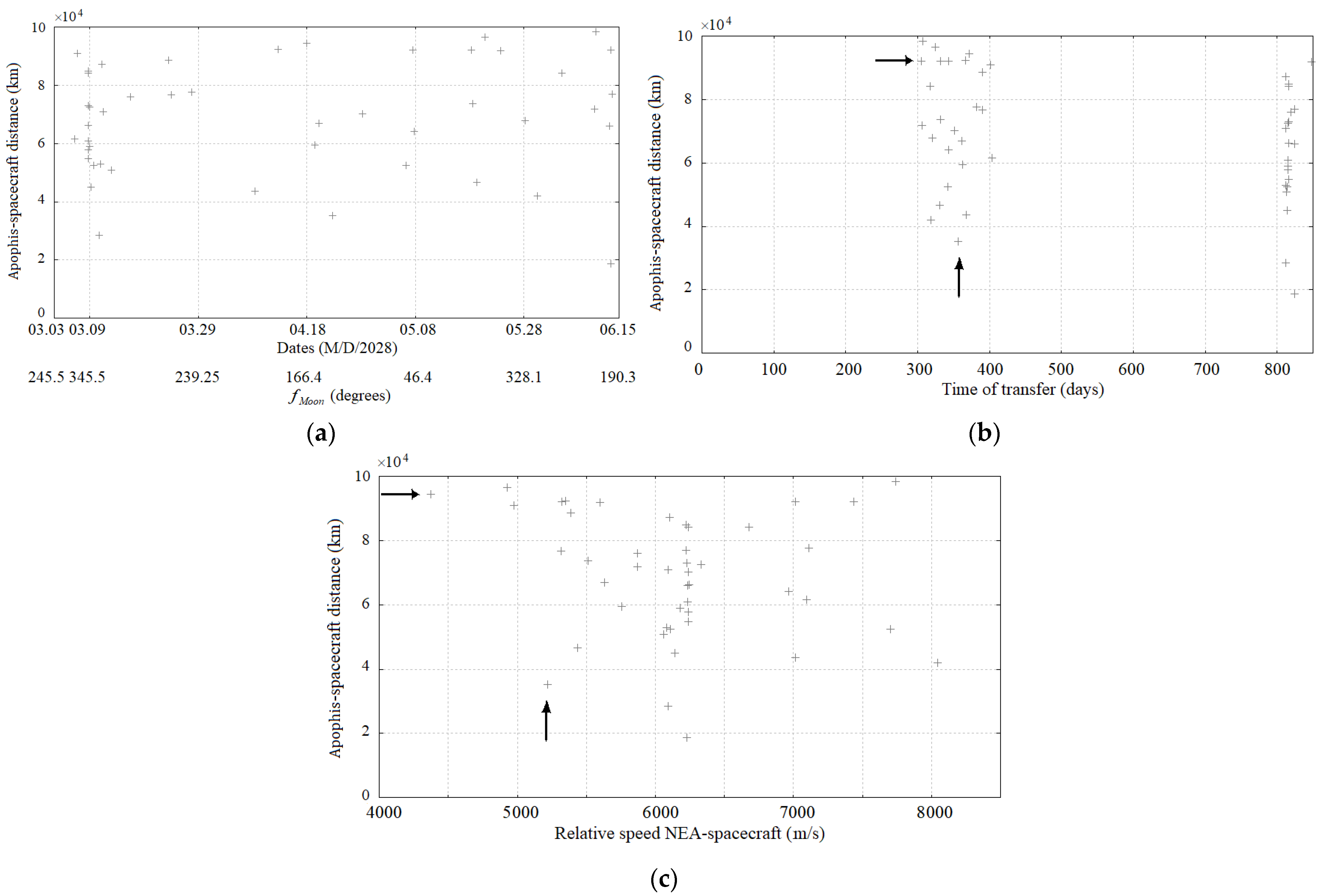
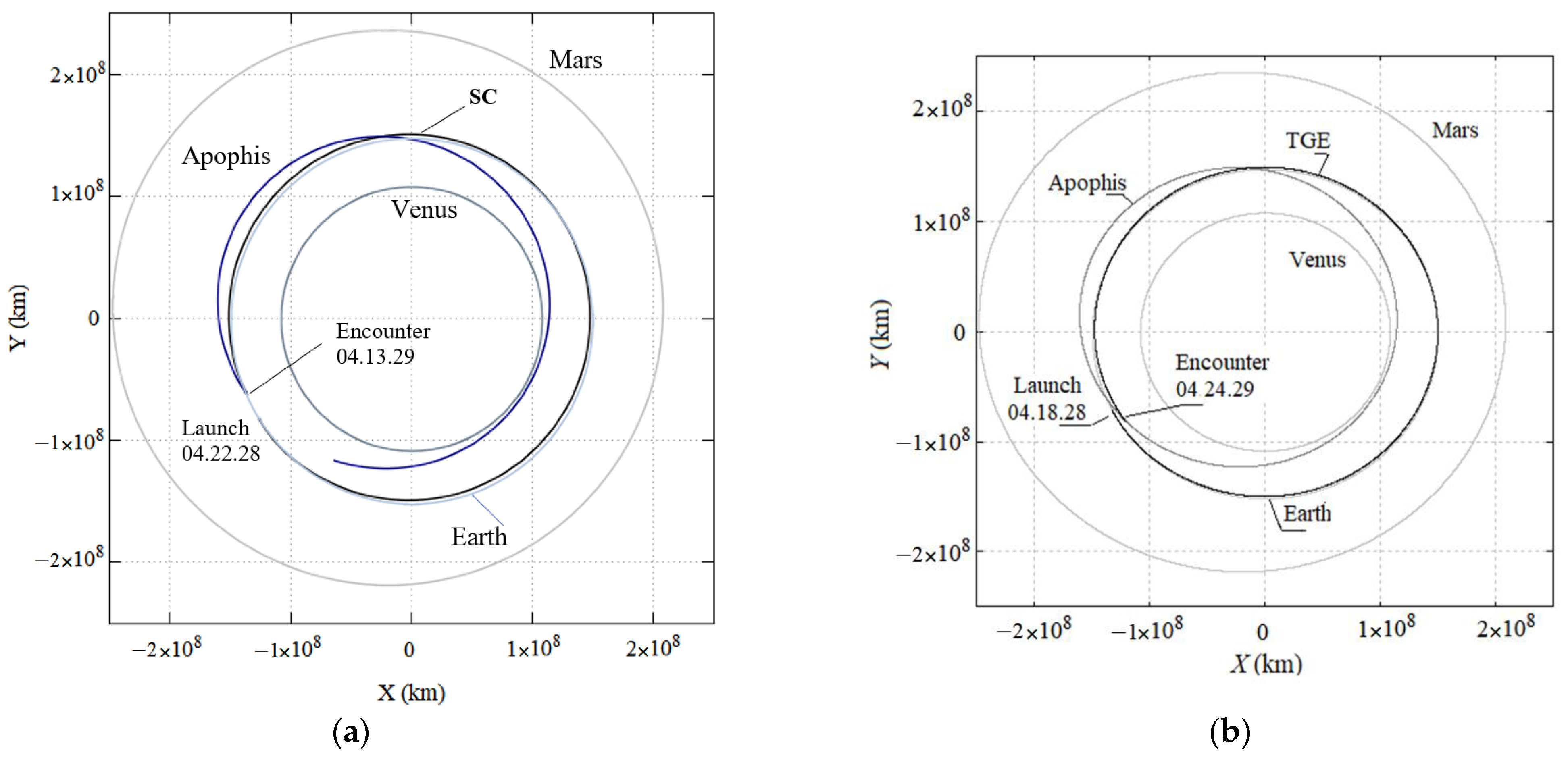
4.3.2. Transfer to the 99942 Apophis

Orbits of the Aten class spend most of their orbital period, or all of it, inside the primary interception region due to the values of their semimajor axes and eccentricities. As a result, the launch windows for TGEs are almost continuous, and a larger number of solutions can be found for transfers to NEAs belonging to the Aten class via TGEs with CPA below 10⁵ km without applying ΔVs for correction maneuvers. For example, considering a launch window from 03.03.2028 to 06.27.2028 and the steps described in Section 4.2, an analysis of the NEA-spacecraft distance diagrams only makes sense when this quantity is less than 10⁵ km, as shown in Figure 13a. Note that there are solutions with NEA–spacecraft distance of less than 10⁵ km for the entire launch window interval.

To find the best transfer, the time of flight and the NEA–spacecraft relative speed need to be analyzed. To drive the search, the NEA–spacecraft distance as a function of time of flight, shown in Figure 13b, and as a function of the NEA–spacecraft relative speed, as shown in Figure 13c, are considered. Comparing these figures, the two TGEs with the shortest NEA–spacecraft distance at CPA have the longest transfer times (over 800 days) and relative speeds of the order of 6000 m/s. Excluding these two solutions, the choice falls to the TGE with the fourth-lowest NEA–spacecraft relative speed (5220 m/s), third-lowest NEA–spacecraft distance (35,228.87 km), and the TGE with the lowest NEA–spacecraft relative speed (4373 m/s); however, the latter has an NEA–spacecraft distance of 94,512.43 km. Both are indicated with arrows in Figure 13.

Table 3. Properties of the Earth-NEA 99942 Apophis transfer (first solution).

Property	First Transfer	Second Transfer
Launch window M/D/Y	03/03/28 to 06/27/28	03/03/28 to 06/27/28
Launch date M/D/Y	6 h 04/06/28	12 h 04/18/28
Circular parking LEO altitude (km)	200 km
VSC (m/s)	10,932.494	10,935.384
|ΔVTGE | (m/s)	3150.567	3153.458
|ΔV| at aphelion (m/s)	20	18
|ΔVLaunch| (reference) Lambert’s Meth. * (m/s)	3331
Launch C3 relative to the Earth (106 m2/s2)	−1.597	−1.534
Impact date, M/D/Y	04/13/2029	04/24/2029
Time of transfer (days)	356.69	371.39
Distance from Earth at impact (km)	24,184,985	28,267,878
Arrival Impact Angles (degrees)	22.27	7.57
Relative velocity at impact (m/s)	5220.245	4373.068

* Without middle-way correction maneuvers.

presents the parameters of these transfers and Figure 14 shows these two TGEs with highlights of their launches from the Earth and encounters with the Apophis.

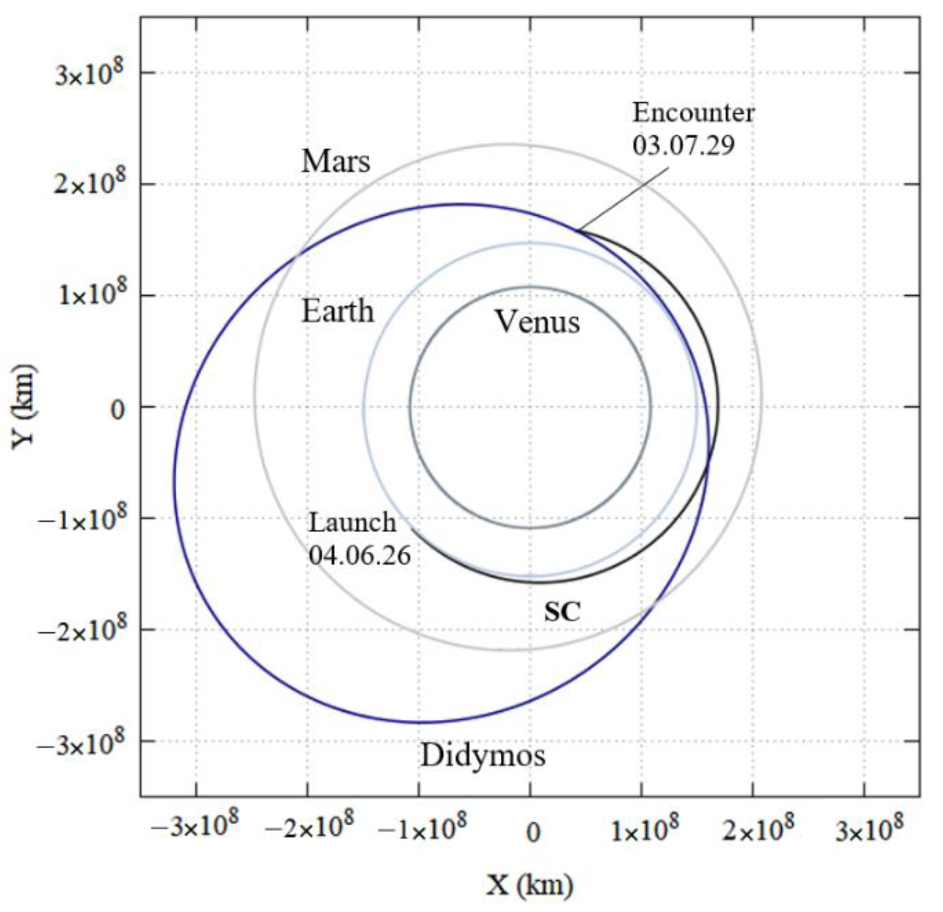
4.3.3. Transfer to the 65803 Didymos

Didymos will penetrate the primary interception region on 2 November 2026. Subtracting the half orbital period of the reference ellipse, the beginning of the launch window is found on 6 March 2026, and as the passage for this region is fast, the launch window closes on 29 April 2026.

Table 4. Properties of the Earth-NEA Didymos transfer.

Launch Window M/D/Y	03/06/26 to 04/29/26
Launch date M/D/Y	6 h 04/06/26
Circular parking LEO altitude (km)	200
VSC (m/s)	10,932.389
|ΔVTGE | (m/s)	3144
|ΔV| at perihelion (m/s)	22
|ΔVLaunch| (reference) Lambert’s Meth. * (m/s)	3318
Launch C3 relative to the Earth (106 m2/s2)	−1.796
Impact date, M/D/Y	03/07/2029
Time of transfer (days)	1086
Distance from Earth at impact (km)	19,126,666
Arrival Impact Angles (degrees)	15.04
Relative velocity at impact (m/s)	9240.300

* Without middle-way correction maneuvers.

presents the parameters of the transfer with CPA of 83,904 km, which is overcome with a |ΔV| of 22 m/s at the perihelion of the selected TGE. Figure 15 shows the TGE with highlights of their launches from the Earth and encounters with Didymos.

5. Conclusions

From a set of periodic orbits around the Lagrangian equilibrium point L₁, called family G, predicted by the circular Restricted Three-Body Problem, studies on collisions with the Moon, escape from the Earth–Moon system, and far-reaching geocentric trajectories derived from these periodic orbits were presented. Among these, we highlighted the escape trajectories (named TGEs) whose ranges allow for the planning of missions to Near-Earth Asteroids.

One of the main features of the escape trajectories (TGEs) is the departure from the Earth with C₃ (characteristic energy) < 0 and, therefore, a |ΔV_TG| at launch for altitudes between 200 km and 1000 km is 2.5% to 5% lower than required to generate direct escape geocentric parabolas (C₃ = 0) and up to 5% lower than the value required for transfers to NEAs obtained by conventional methods such as Lambert’s method. Since they are derived from the periodic orbits of family G, the escape trajectories make a passage through the Moon, collide, or perform swing-bys. In the latter case, the swing-bys guarantee the necessary energy gain to make C₃ relative to the Earth positive and send the spacecraft into interplanetary space, called TGEs, or to generate geocentric trajectories with an apogee between 9 × 10⁵ km and 2 × 10⁶ km. The latter are called TGIs.

Studies on launch speeds (V_SC) required to generate collision (TGCs), escape (TGEs), and inversion (TGIs) trajectories and their dependence on the circular LEO altitudes (h₀), ${\Omega }_{Moon}$, and f_Moon, as well as the ranges of their final heliocentric orbits, were also presented. These studies led to a methodology for planning transfers to NEAs.

Finally, missions to the NEAs 3361 Orpheus (Apollo class), 99942 Apophis (Aten class), and Didymos (Apollo class) were studied. They show how launch windows are determined and how missions are investigated. The costs of these missions were analyzed in terms of |ΔVs| needed to launch and correct the TGEs until impact with NEAs, which fall below those required to generate parabolic geocentric escape trajectories and interplanetary trajectories by Lambert’s method. Thus, transfers planned via TGEs can be classified as low-cost missions.

In forthcoming works, powered lunar and Earth swing-bys from the TGIs could be planned to generate more far-reaching escape trajectories capable of achieving or crossing the orbits of Venus and Mars, for example.

References

1. Minor Planet Center. “Latest Published Data,” 2022. Available online: https://www.minorplanetcenter.net/mpc/summary (accessed on 30 March 2022).
2. Shoemaker, E.M.; Williams, J.G.; Hellin, E.F.; Wolfe, R.F. Orbital Classes, Collision Rates with Earth, and Origin; Asteroids, T.G., Ed.; University of Arizona Press: Tucson, AZ, USA, 1979; pp. 253–282. [Google Scholar]
3. Broucke, R.A. Periodic orbits in the restricted three body problem with earth-moon masses. Tech. Rep. 1968. [Google Scholar]
4. de Melo, C.; Macau, E.; Winter, O.; Neto, E.V. Alternative paths for insertion of probes into high inclination lunar orbits. Adv. Space Res. 2007, 40, 58–68. [Google Scholar] [CrossRef]
5. de Melo, C.F.; Macau, E.E.N.; Winter, O. Strategies for plane change of Earth orbits using lunar gravity and derived trajectories of family G. Celest. Mech. Dyn. Astron. 2009, 103, 281–299. [Google Scholar] [CrossRef]
6. De Melo, C.F.; Macau, E.E.N.; Winter, O.C. Alternative Transfers to the NEOs 99942 Apophis, 1994 WR12, and 2007 UW1 via Derived Trajectories from Periodic Orbits of Family G. Math. Probl. Eng. 2009, 2009, 303604. [Google Scholar] [CrossRef]
7. Salazar, F.J.T.; de Melo, C.F.; Macau, E.E.N.; Winter, O. Three-body problem, its Lagrangian points and how to exploit them using an alternative transfer to L4 and L5. Celest. Mech. Dyn. Astron. 2012, 114, 201–213. [Google Scholar] [CrossRef]
8. Turco, R.; Toon, O.; Park, C.; Whitten, R.; Pollack, J.; Noerdlinger, P. An analysis of the physical, chemical, optical, and historical impacts of the 1908 Tunguska meteor fall. Icarus 1982, 50, 1–52. [Google Scholar] [CrossRef]
9. Shoemaker, E.M. Asteroid and comet bombardment of the Earth. Annu. Rev. Earth Planet. Sci. 1983, 11, 461–494. [Google Scholar] [CrossRef]
10. Kerr, R.A. Huge impact tied to mass extinction. Science 1992, 257, 878–880. [Google Scholar] [CrossRef]
11. Popova, O.P.; Jenniskens, P.; Emel’yanenko, V.; Kartashova, A.; Biryukov, E.; Khaibrakhmanov, S.; Shuvalov, V.; Rybnov, Y.; Dudorov, A.; Grokhovsky, V.I.; et al. Chelyabinsk airburst, damage assessment, meteorite recovery, and characterization. Science 2013, 342, 1069–1073. [Google Scholar] [CrossRef] [Green Version]
12. The Guardian. Scientists Reveal the Full Power of the Chelyabinsk Meteor Explosion. 2013. Available online: https://www.theguardian.com/science/2013/nov/06/chelyabinsk-meteor-russia#:~:text=Travelling%20at%20a%20speed%20of,knock%20people%20off%20their%20feet (accessed on 23 May 2022).
13. Chapman, C.R. Space weathering of asteroid surfaces. Annu. Rev. Earth Planet. Sci. 2004, 32, 539–567. [Google Scholar] [CrossRef] [Green Version]
14. Prockter, L.; Murchie, S.; Cheng, A.; Krimigis, S.; Farquhar, R.; Santo, A.; Trombka, J. The NEAR shoemaker mission to asteroid 433 eros. Acta Astronaut. 2002, 51, 491–500. [Google Scholar] [CrossRef]
15. Kawaguchi, J.; Fujiwara, A.; Uesugi, T. Hayabusa—Its technology and science accomplishment summary and Hayabusa-2. Acta Astronaut. 2008, 62, 639–647. [Google Scholar] [CrossRef]
16. Tsuda, Y.; Saiki, T.; Terui, F.; Nakazawa, S.; Yoshikawa, M.; Watanabe, S.-I. Hayabusa2 mission status: Landing, roving and cratering on asteroid Ryugu. Acta Astronaut. 2020, 171, 42–54. [Google Scholar] [CrossRef]
17. Lauretta, D.S.; Balram-Knutson, S.S.; Beshore, E.; Boynton, W.V.; D’Aubigny, C.D.; DellaGiustina, D.; Enos, H.L.; Gholish, D.R.; Hergenrother, C.W.; Howell, E.S.; et al. OSIRIS-REx: Sample Return from Asteroid (101955) Bennu. Space Sci. Rev. 2017, 212, 925–984. [Google Scholar] [CrossRef] [Green Version]
18. NASA. NASA, SpaceX Launch DART: First Test Mission to Defend Planet Earth. 2021. Available online: https://www.nasa.gov/press-release/nasa-spacex-launch-dart-first-test-mission-to-defend-planet-earth (accessed on 19 April 2022).
19. Michel, P.; Cheng, A.; Küppers, M.; Pravec, P.; Blum, J.; Delbo, M.; Green, S.F.; Rosenblatt, P.; Tsiganis, K.; Vincent, J.; et al. Science case for the Asteroid Impact Mission (AIM): A component of the Asteroid Impact & Deflection Assessment (AIDA) mission. Adv. Space Res. 2016, 57, 2529–2547. [Google Scholar]
20. Scheirich, P.; Pravec, P.; Thomas, C.A. Observations of Didymos in support of DART and Hera. EPSC-DPS Jt. Meet. 2019, 2019, EPSC-DPS2019. [Google Scholar]
21. Lawden, D.F. Perturbation maneuvers. J. Br. Interplanet Soc. 1954, 13, 329–334. [Google Scholar]
22. Minovitch, M. A method for determining interplanetary free-fall reconnaissance trajectories. JPL Tec. Memo. 1961, 312, 130. [Google Scholar]
23. Broucke, R. The celestial mechanics of gravity assist. Astrodyn. Conf. 1988, 69–78. [Google Scholar]
24. Dunham, D.; Davis, S. Optimization of a multiple lunar-swingby trajectory sequence. Astrodyn. Conf. 1985, 1978. [Google Scholar] [CrossRef]
25. Prado, F.B.A. Orbital control of a satellite using the gravity of the moon. J. Braz. Soc. Mech. Sci. Eng. 2006, 28, 105–110. [Google Scholar] [CrossRef] [Green Version]
26. Farquhar, R. Detour to a Comet; Journey of the International Cometary Explorer. Planet. Rep. 1985, 5, 4–6. [Google Scholar]
27. NASA Science. ISEE-3/ICE. 24 July 2019. Available online: https://solarsystem.nasa.gov/missions/isee-3-ice/in-depth/ (accessed on 22 September 2021).
28. Kawaguchi, J. On the lunar and heliocentric gravity assist experienced in the planet-b (‘nozomi’). Fourth Int. Symp. Space Flight Dyn. Iguassu Falls Braz. 1999, 8–12. [Google Scholar]
29. Kawaguchi, J.; Nakatani, I.; Uesugi, T.; Tsuruda, K. Synthesis of an alternative flight trajectory for Mars explorer, Nozomi. Acta Astronaut. 2003, 52, 189–195. [Google Scholar] [CrossRef]
30. National Aeronautics and Space Administration. “Nozomi,” NASA Space Science Data Coordinated Archive. Available online: https://nssdc.gsfc.nasa.gov/nmc/spacecraft/display.action?id=1998-041A (accessed on 22 September 2021).
31. Dunham, D.W.; Guzmán, J.J.; Sharer, P.J. STEREO trajectory and maneuver design. Johns Hopkins APL Tech. Dig. 2009, 28, 104–125. [Google Scholar]
32. Ocampo, C. Trajectory analysis for the lunar flyby rescue of AsiaSat-3/HGS-1. Ann. N. Y. Acad Sci. 2005, 1065, 232–253. [Google Scholar] [CrossRef]
33. Murray, C.D.; Dermott, S.F. Solar System Dynamics; Cambridge University Press: Cambridge, UK, 1999. [Google Scholar]
34. Stroemgren, E. Connaissance actuelle des orbites dans le probleme des trois corps. Publ. Og Mindre Meddeler Fra Kbh. Obs. 1933, 100, 1–44. [Google Scholar]
35. Jet Propulsion Laboratory (JPL). Horizons System. Available online: https://ssd.jpl.nasa.gov/horizons/ (accessed on 15 May 2022).
36. Jet Propulsion Laboratory (JPL). Horizons Web Application. Available online: https://ssd.jpl.nasa.gov/horizons/app.html#/ (accessed on 23 May 2022).
Figure 1. A periodic orbit of family G obtained by numerical integration by taking x0 = 0.04999999 and y ˙ 0 = 5.458017660 at t0 = 0 in Equation (1): (a) In the synodic frame (x,y,z), and the Lagrangian equilibrium points associated with the Earth–Moon system; (b) same periodic orbit and the Moon’s orbit in a geocentric frame (ξ, η, ζ).
Symmetry 14 01132 g001
Figure 2. Relative positioning between the Sun, the Earth, a spacecraft (SC), and the Moon at the instant the spacecraft is inserted into a trajectory derived from a periodic orbit of family G (t0 = 0), in BC4BP (non-scale).
Symmetry 14 01132 g002
Figure 3. Curves VSC × fMoon for Ω M o o n = 0 at t0 = 0 and fEarth ranging from 0 to 26.92846°: (a) h0 = 200 km; (b) h0 = 700 km; (c) VSC × fMoon × Ω M o o n ( Ω M o o n = 0°, 30°, 60°, 90°, 120° and 150°) at t0 = 0, upper right corner surface: VSC = f ( Ω M o o n , fMoon) for first TGC generated by Equation (4). From the bottom upwards, the first curve is the first TGC, the second curve is the first TGE, the third is the last TGE, and the fourth is the last TGI.
Symmetry 14 01132 g003
Figure 4. Trajectories G: (a) Collision—TGC, (b) direct escape—TGE, (c) inversion—TGI and the Moon’s orbit obtained for fMoon = Ω M o o n = 0 and fEarth = 0, at t0 = 0, as seen in a geocentric reference frame (ξ, η, ζ;).
Symmetry 14 01132 g004
Figure 5. (a) VSC (yellow) and escape speed; (b) speed of circular orbits Vcir; (c) | Δ V T G | (green) to generate trajectories G and | Δ V e s c | .
Symmetry 14 01132 g005
Figure 6. Specific orbital energy of the TGEs and TGIs relative to the Earth (Δε24) as a function of (a) Ψ, (b) VSC, and (c) periselene radius as a function of Ψ. All graphics obtained for h0 = 200 km, Ω M o o n = fMoon = fEarth = 0 at t0 = 0.
Symmetry 14 01132 g006
Figure 7. TGs’ specific orbital energy relative to the Sun (Δε14) as a function of (a) Ψ and (b) VSC. All graphics obtained for h0 = 200 km, Ω M o o n = fMoon = 0 at t0 = 0.
Symmetry 14 01132 g007
Figure 8. Distribution of perihelia and aphelia for (a) internal TGEs and (b) external TGEs.
Symmetry 14 01132 g008
Figure 9. TGEs with the smallest perihelion (internal TGE) and largest aphelion (external TGE).
Symmetry 14 01132 g009
Figure 10. An illustration of the primary intercepting region (between the external and internal circumferences), reference ellipse, and launch window for an NEA whose orbit crosses the external circumference.
Symmetry 14 01132 g010
Figure 11. VSC × fMoon and the launch window. (a) First launch window from 02/15/2025 to 05/08/2025, (b) second launch window from 07/01/2025 to 07/30/2025.
Symmetry 14 01132 g011
Figure 12. TGEs and the orbits of Earth, Venus, Mars, and 3361 Orpheus for (a) first launch window from 02/15/2025 to 05/08/2025—first solution, (b) first launch window—second solution, and (c) second launch window from 07/01/2025 to 07/30/2025.
Symmetry 14 01132 g012
Figure 13. Apophis-spacecraft distance diagrams limited to 104 km: (a) as a function of fMoon and the launch window 03/03/2028 to 06/15/2028, (b) as a function of time of transfer, (c) as a function of relative Apophis-spacecraft speed.
Symmetry 14 01132 g013
Figure 14. TGEs and the orbits of the Earth, Venus, Mars, and 99942 Apophis for (a) first solution with launch on 04/22/2028 and encounter on 04/13/2029 and (b) second solution with launch on 04/18/2028 and encounter on 04/24/2029.
Symmetry 14 01132 g014
Figure 15. TGE and the orbits of the Earth, Venus, Mars, and Didymos for launch on 04/06/2026 and encounter on 03/07/2029.
Symmetry 14 01132 g015