1. Introduction
It is frequently recognized that graphs are basically representations of relations. A graph is a useful means of describing information concerning object relationships. Vertices represent objects, while edges describe relationships.
It can be used to look at combinatorial problems in a lot of different fields, such as algebra, topology, zoology, number theory, geometry, and image capture and clustering.
The graph’s vertices and edges are used to describe objects and the relationships between them, respectively. Vagueness in global issues can emerge in the information that specifies the conditions. FG models are useful mathematical tools for dealing with combinatorial issues in different fields, such as topology, algebra, optimization, computers, and environmental science. Because of the inherent presence of vagueness and ambiguity, FG models are more complex in comparison to simple graphical models. The first time fuzzy set theory was used, it was used to deal with a lot of complicated situations that did not have enough information.
Zadeh [
1] proposed the theory of a fuzzy set (FS), which is applicable in several areas, and his FS has a true membership function which is limited to [0,1]. In approximate reasoning, the importance of fuzzy theory is particularly significant in overcoming combinatorial challenges in numerous domains, such as algebra, image segmentation, topology, operational research, medical science, and algebraic structure. Rosenfeld [
2] discussed the fuzzy versions of various graph-based theories. Ghorai and Pal [
3,
4] recently studied the extensions of FG, such as bipolar fuzzy graphs,
m-polar fuzzy planner graphs, and
m-polar fuzzy graphs. They defined the density of
m-polar fuzzy graph techniques as well as a set of operations. Nagoor Gani and Radha [
5] discussed a few operations on regular FG. Mathew and Sunitha described some kinds of arcs of FG. Bhattacharya [
6] gave some remarks on FG. Atanassov [
7] extended the FS to the intuitionistic fuzzy set. Shao et al. [
8] developed new notions of the bondage number in intuitionistic fuzzy graphs. Rashmanlou et al. [
9,
10] discussed briefly a bipolar fuzzy graph with the product of bipolar fuzzy graphs, categorical operations, and related degrees. Rashmanlou et al. [
11] were interested in research on interval-valued fuzzy graphs. Zeng et al. [
12] invented different properties for single-valued neutrosophic graphs. Shao et al. [
13] studied the properties of vague graphs.
Ramot et al. [
14] proposed the notion of a “CFS” in 2002. CFSs are an innovative development of Zadeh’s fuzzy sets. Despite all of the benefits of this theory, we still face enormous challenges when attempting to counter various physical conditions using a true membership function. Because of this, it is very important to add a new step to fuzzy set theory that takes into account complex numbers, which are an expansion of real numbers. Complex fuzzy logic is a linear extension of standard fuzzy logic. It lets problems in fuzzy logic that cannot be solved with a simple membership function grow and change in a natural way. This specific set plays a critical role in a variety of executions, particularly intelligent control systems and the prediction of periodic phenomena, where various fuzzy variables are connected in a complicated way that cannot be accurately represented by simple fuzzy operations. Furthermore, these sets are employed to tackle a variety of difficulties, particularly the various periodic aspects and forecasting challenges. One of the far-reaching implications of researching the CFS is that it effectively illustrates data with uncertainty and periodicity. Buckley described fuzzy complex numbers in [
15]. Yaqoob et al. [
16] studied the complex intuitionistic fuzzy graph and the complex neutrosophic graph. Shoaib et al. [
17] proposed the concept of a complex Pythagorean fuzzy graph. Shoaib et al. [
18] discussed some properties, symmetric difference and maximal product of picture fuzzy graphs. Gulzar et al. [
19,
20,
21] discussed fuzzy groups.
The CFG is the generalization of the FG. We define the order and size of CFG. Furthermore, we present the degree of vertex and total degree of vertex concepts for CFG. We describe some basic properties, including the join, union, and complement of CFG. We discuss some new operations with maximal product and symmetric difference on CFG with elaboration of examples and related theorems. Lastly, we analyze the application of CFG.
3. CFGs
This section presents the idea of complex fuzzy relations and CFG, as well as some of their properties.
Definition 4. A CFG on a universe Y with underlying set A is an ordered pair ; Q is a complex fuzzy set on A and L is a complex fuzzy set on such that, and ∈ ∀ x, y ∈ A.
Definition 5. Let , ,
, be the three CFSs in Y:
- (i)
if and only if for amplitude terms and for phase terms, ∀ x ∈ Y.
- (ii)
if and only if for amplitude terms and for phase terms, ∀ x ∈ Y.
For simplicity, is called the complex fuzzy number where μ ∈ [0,1], and α ∈ .
Definition 6. Let and be the two complex picture fuzzy sets in Y, then
- (i)
∪ =.
- (ii)
∩ =.
Definition 7. A complex fuzzy set L in Y × Y is called a complex fuzzy relation in Y, characterized by × Y}, where : Y × Y → [0,1] depicts the membership function of L and ∈∀ xy ∈ Y × Y.
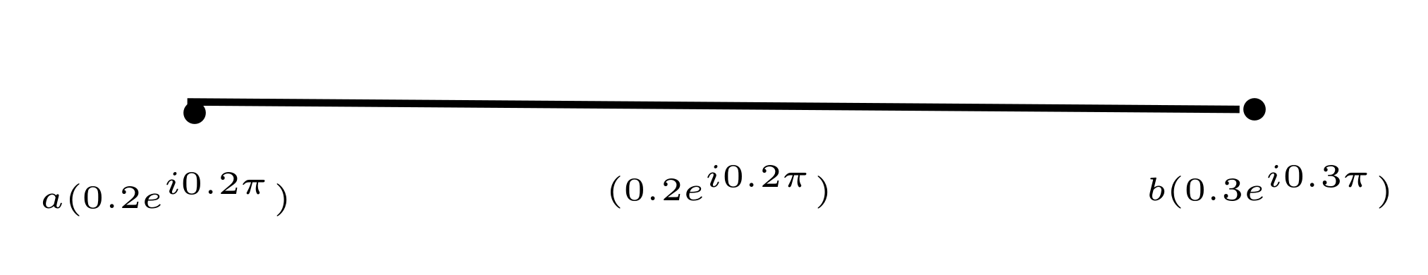
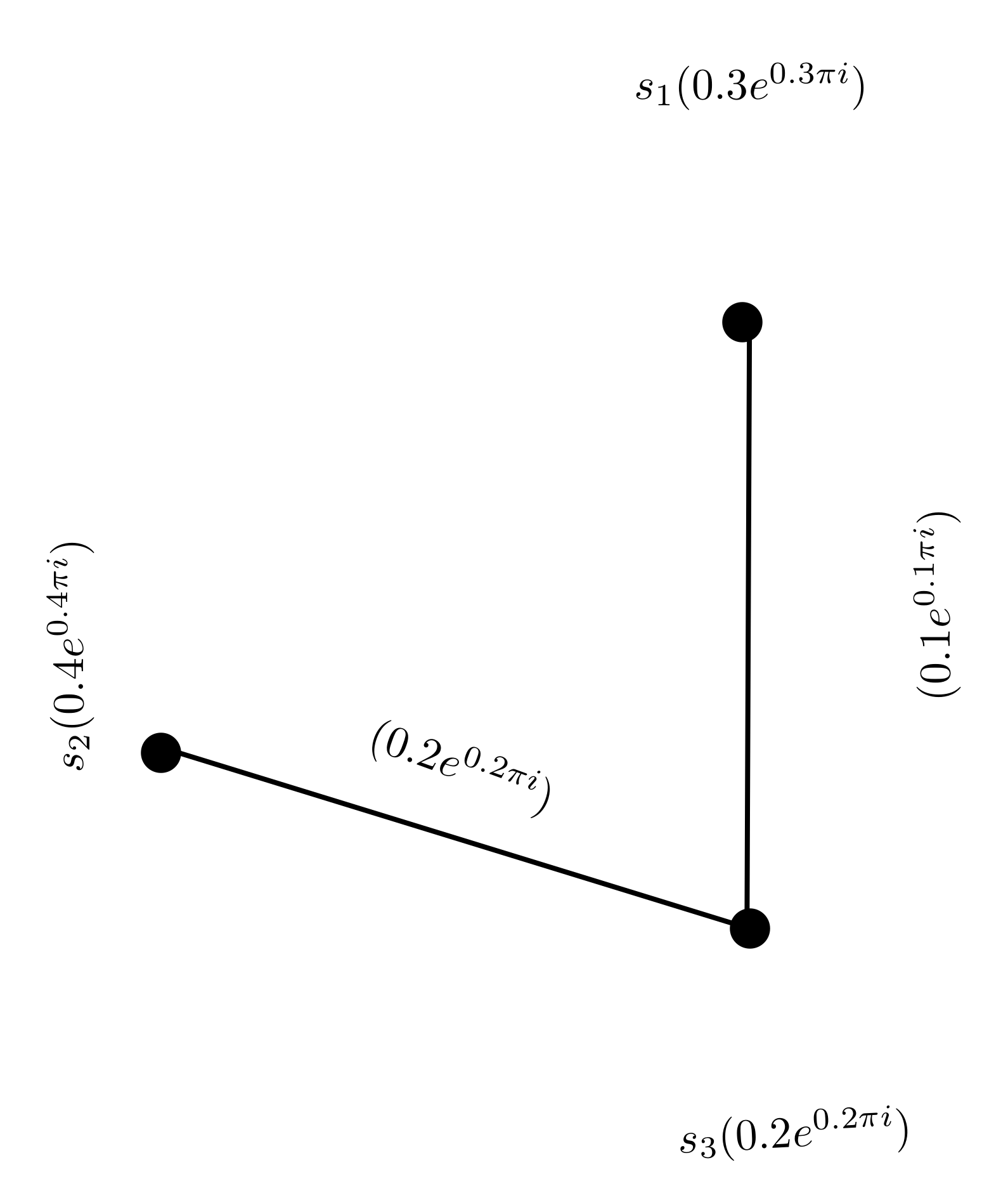
Example 1. Let G = (A,B) be a graph with as the vertex set and as the edge set of G. is a CFG on A, as given in Figure 1, defined by .
Definition 8. Let and be the vertex set and edge set of a CFG τ, then the order of a CFG τ is denoted by O(τ) and is defined as O(τ) = .
The size of a CFG τ is denoted by S(τ ) and is defined as S(τ) = .
Example 2. The order and size of the CFG given in Figure 1 is O(τ) = and S(τ) = , respectively. Definition 9. The complement of a CFG τ = (Q,L) on the underlying graph G = (A,B) is a CFG = (,) defined by
- 1.
=
- 2.
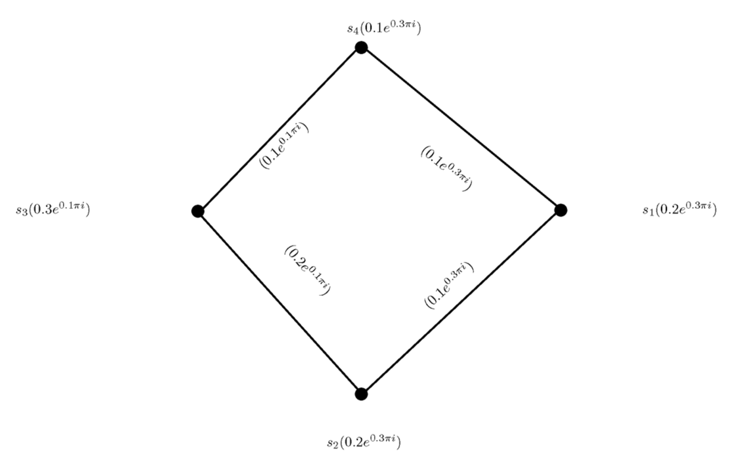
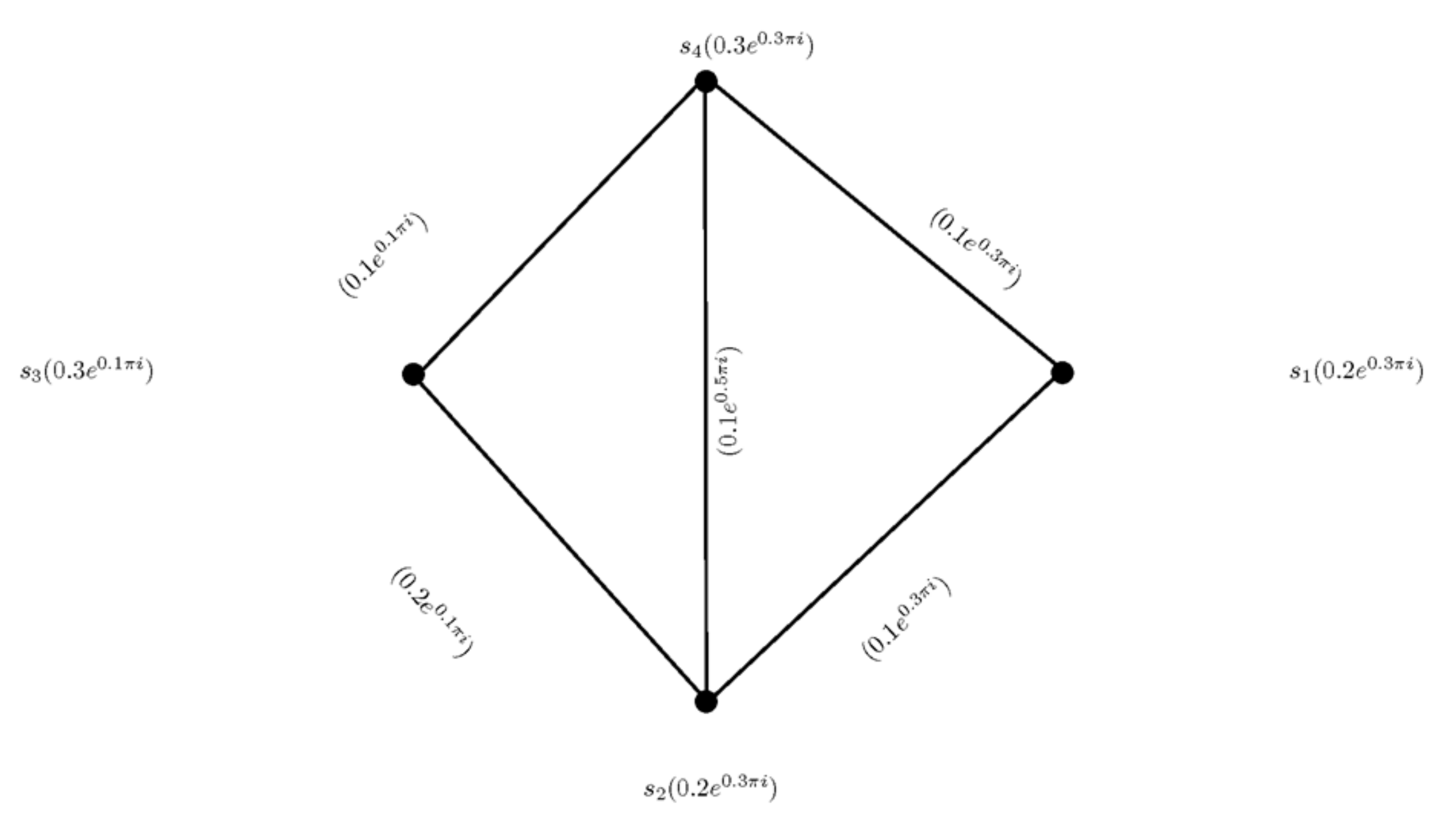
Example 3. Consider a CFG τ = (Q,L) on , which is shown as in Figure 2 where , . Utilizing the Definition 9, the complement of a CFG can be obtained, which is shown as in Figure 3. Where .
It is easy to see from Figure 3 that = is a CFG. Theorem 1. The complement of a complement of CFG is a CFG itself, that is, = τ
Proof. Suppose that is a CFG. Then, by utilizing Definition 9.
= = for all x ∈ A
if then
=
=
if then
= −
= −
=
for all x, y ∈ A. Hence = . □
Definition 10. The union τ∪τ = of two CFGs τ = and τ = of the graphs = and = , respectively, is defined as follows: (x) Definition 11. The ring-sum τ⊕τ = of two CFGs τ = and τ = of the graphs and , respectively, is defined as follows:
=(, Definition 12. Let τ = and τ = be two CFGs of and , respectively. The join ττ = of τ = and τ = , defined as
- (i)
=(,
- (ii)
=(,
- (iii)
= where is the arcs set joining the nodes of and , .
Definition 13. The degree of a vertex x ∈ A in a CFG τ stands for , and is described as = , where =
Definition 14. The total degree of a vertex x ∈ A in a CFG τ stands for , and is described as = , where = +
Definition 15. Let τ and τ be two CFGs. For any vertex x , there are three cases to consider.
- Case 1:
Either x or x . Then no arc incident at x lies in . Thus, for c ,
= =
= . For x .
= =
= .
- Case 2:
x but no arc incident at x lies in . Then any arc incident at x is either or .
=
= +
= +
= +
= + +
= + +
= +
- Case 3:
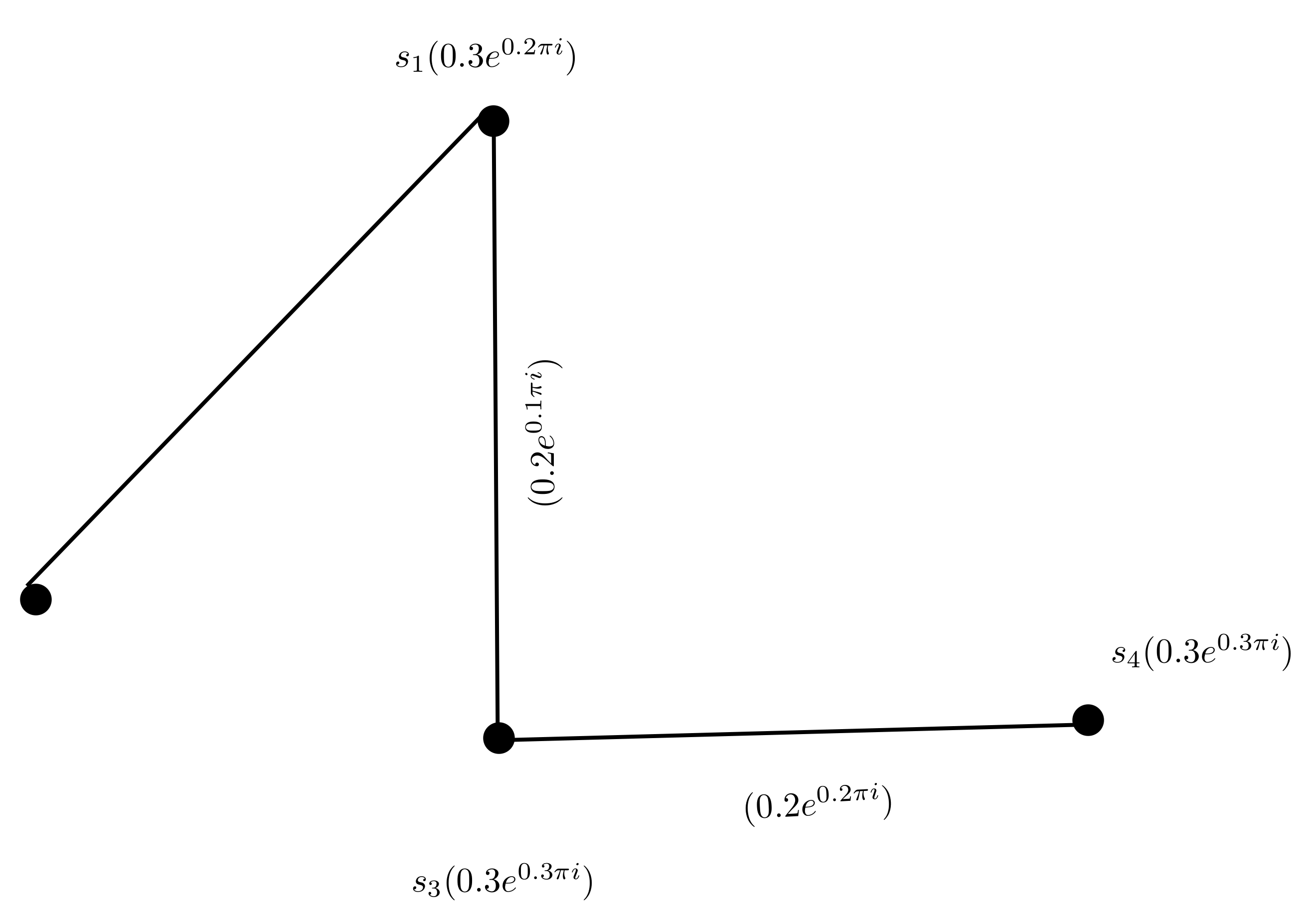
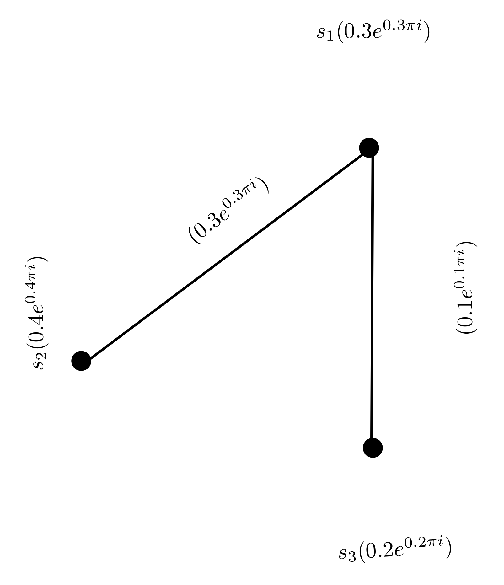
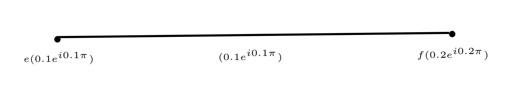
Example 4. Suppose that and are two CFGs on and , respectively, as shown in Figure 4 and Figure 5. Moreover, is shown in Figure 6. If ∈, then
= =
Therefore, = =
= =
Therefore, = =
Since ∈∩ but there is no edge incident at lies in ,
= + =
Therefore, = + = ()
= + +
=
Since ∈∩ and ∈∩,
= + =
Therefore, =
= +
+ =
Therefore, =
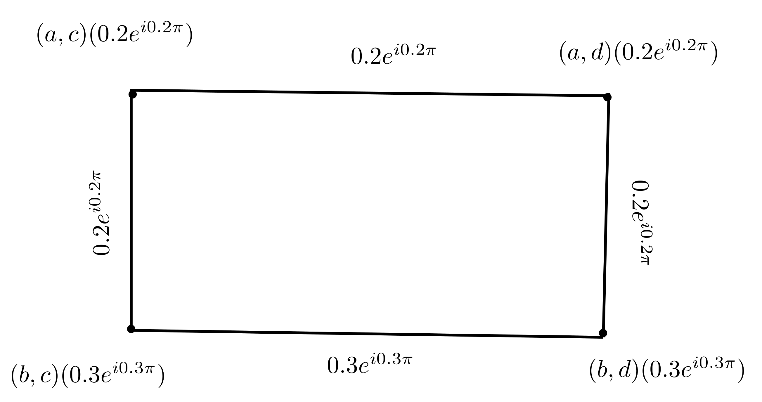
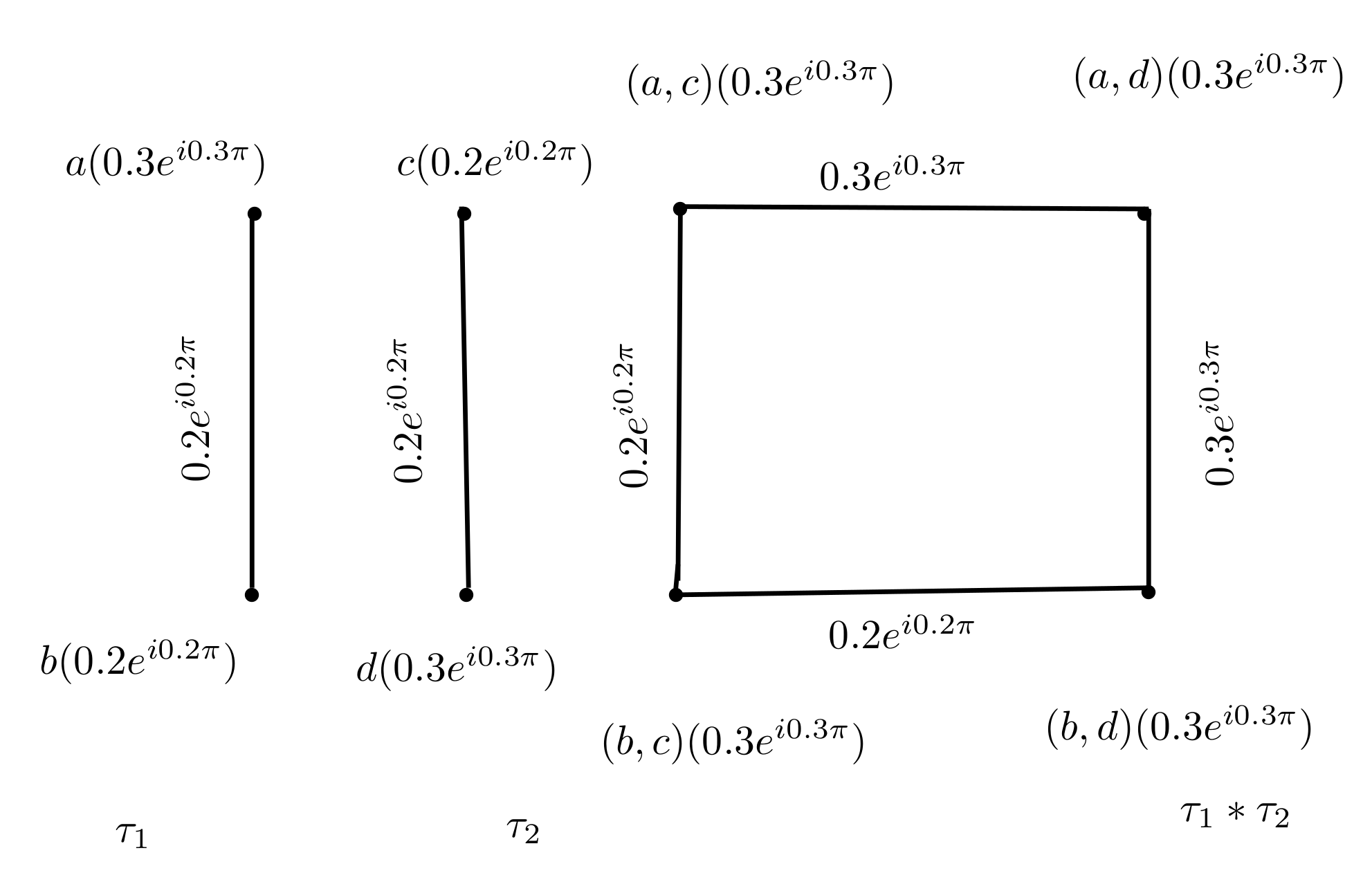
Definition 16. Maximal product of two CFGs and is defined as
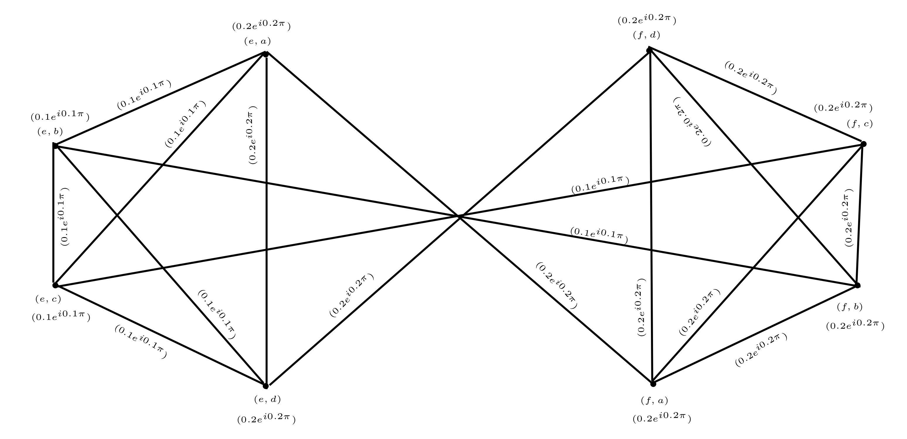
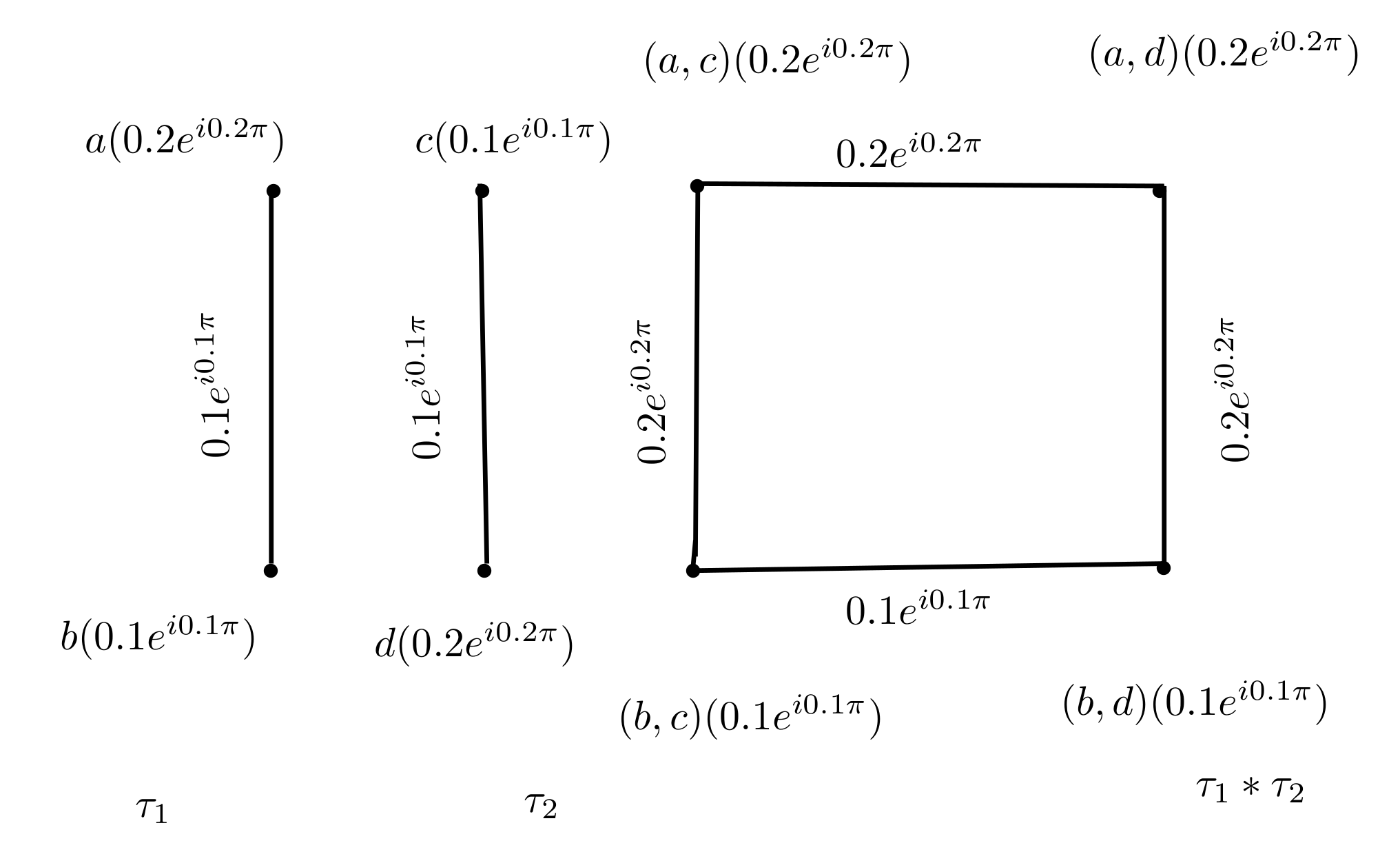
Example 5. Suppose and are two CFGs, shown in Figure 7 and Figure 8. Their maximal product is shown in Figure 9. For vertex (e,a), we find membership value (Mv) as follows:for and . For edge (e,a)(e,b), we find Mv.for and . For edge :for and . Similarly, Mv for all others nodes and edges can be calculated. Proposition 1. Maximal product of two CFGs and , is a CFG.
Proof. Suppose and are two CFGs on crisp graphs
and , respectively and .
We conclude that is a CFG. □
Theorem 2. Maximal product of two strong CFGs and is a strong CFG.
Proof. Suppose and are two strong CFGs on two crisp graphs and .
Hence, is a strong CFG. □
Example 6. Suppose and are two strong CFGs as shown in Figure 10. Hence is also a strong CFG.
Remark 1. If maximal product of two CFGs and is a strong, then and not necessary to be strong, in general.
Example 7. Suppose and are two CFGs as in Figure 11 and Figure 12. We can see that the maximal product of two CFGs and , that is in Figure 13. Then and are strong CFGs, but is not strong. Since = , on other hand = = .
Hence .
Remark 2. The maximal product of two complete CFGs may or may not be a complete CFG because and do not exist in the definition of the maximal product of two CFGs.
Definition 17. Suppose and are two CFGs. Theorem 3. Suppose and are two CFGs. If , and . Then for every
=
Example 8. Take the CFGs , , and as in Figure 14. Since , , , , by Theorem 3.8, we have the following. We conclude from the above calculations that ”the degrees of nodes determined by using the formula of the above theorem and by the directed method are equal”.
Definition 18. Let and be two CFGs. Theorem 4. Suppose and are two CFGs. If , and , . Then for every
= +
Example 9. Let and be two CFGs. If and .
In Example 9, we calculate total degree of nodes of by using Figure 7, Figure 8 and Figure 9. We calculate the total degree of nodes in the maximal product. Choose node (e,a). Similarly, we can calculate it for other nodes.
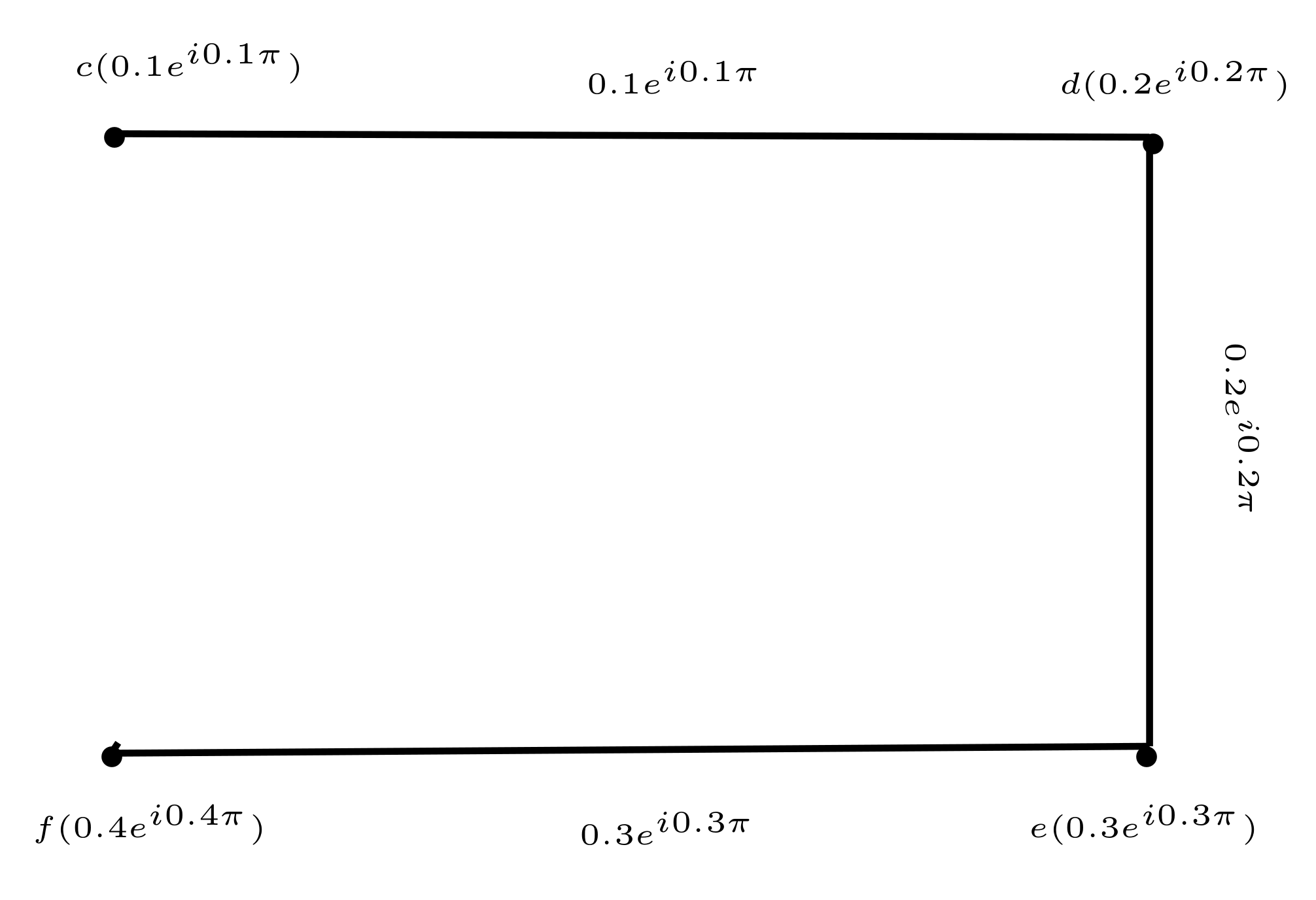
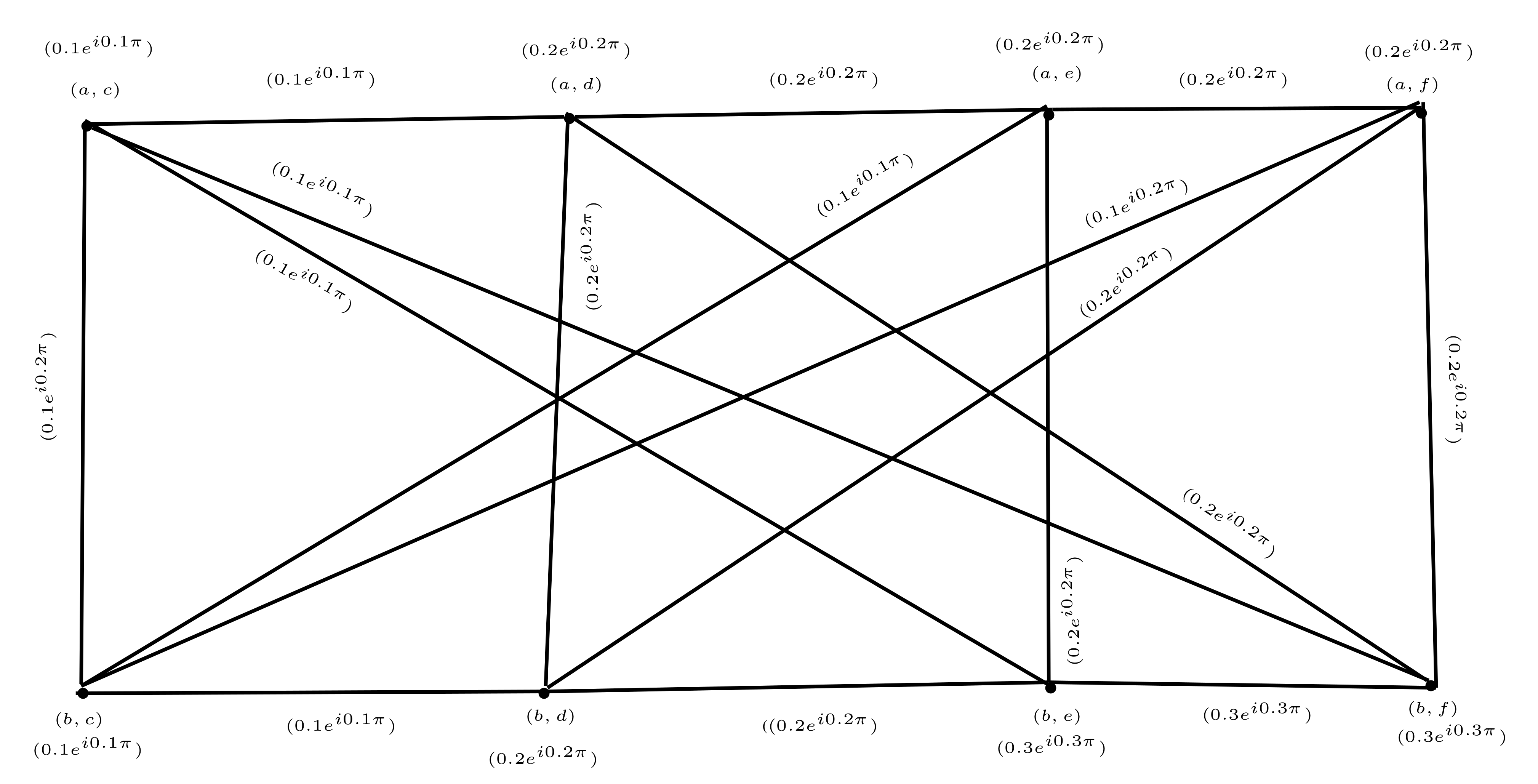
Definition 19. Symmetric difference of two CFGs and is defined as
Example 10. Take and as CFGs as shown in Figure 15 and Figure 16. We can see the symmetric difference of two CFGs and , that is in Figure 17. For node
, we calculate Mv, IDv and NMv as follows:
for
and
.
For arc/edge
, we calculate the Mv.
for
and
.
Now, for edge
we have
for
and
.
We can calculate Mv for all other nodes and edges.
Proposition 2. Symmetric difference of two CFGs and is a CFG.
Proof. Suppose and are two CFGs on two crisp graphs and .
- (i)
- (ii)
- (iii)
If
- (iv)
If
Hence, is a CFG. □
Definition 20. Suppose and are two CFGs. For any node , we have Theorem 5. Suppose and are two CFGs. If and . Then
= q where s= and q= .
Proof. We conclude that = q, where s = and q = . □
Example 11. In Figure 18, , , , and . Then, the total degree of vertex in the symmetric difference is calculated by using the following formula: So, and . Applying the same technique, we can obtain . Now by direct calculations we have: It is obvious from the above calculations that the degrees of nodes determined by using the formula of the above theorem and by the direct method are equal.
Definition 21. Let and be two CFGs. For any vertex , we have Theorem 6. Suppose and are two CFGs. If
Proof.
where value of s and q as follows
s =
and
q =
. □
Example 12. We find the total degree of nodes by using Example 10.
We conclude from the calculations that the total degrees of nodes calculated by the formula of the above theorem and by the direct method are equal.
4. Application of CFG
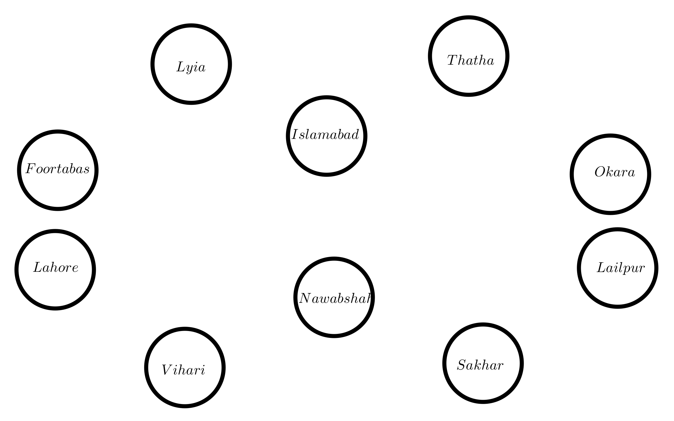
CFGs play a great role in fuzzy decision making and image segmentation. We presented a few factors in the application which will help in a physical way. For this, the government of Pakistan wants to construct COVID-19 Designated Tertiary Hospitals in any district that has a plan to make the minimum number of COVID-19 Designated Tertiary Hospitals in the district so that many people can benefit from this project. For this purpose, the following are some parameters taken into account: (1) a good place to build a COVID-19 Tertiary Hospital; (2) patients; (3) an urban location; (4) access to the facility; (5) security and safety; and (6) cost and efficiency. Assume that members of a team select 10 areas where they are engaged in the established COVID-19 Designated Tertiary Hospitals so that they may assist more patients for their treatment purposes. They see the following two scenarios: Constructing a COVID-19 Designated Tertiary Hospital in 1 of the 10 approved locations.
Constructing a COVID-19 Designated Tertiary Hospital between any 2 of the selected 10 places. Suppose that P = {Islamabad, Thatha, Okara, Lailpur, Sakhar, Nawabshah, Vihari, Lahore, Foortabas, Layia} is the set of locations where the team wishes to construct the COVID-19 Designated Tertiary Hospital as a node set. Assume that, after carefully analyzing the various characteristics, 80 percent of the specialists on the panel agree that Islamabad will have a COVID-19 Designated Tertiary Hospital. As a result, we can determine the term of membership. The phase term, which defines the time, must be computed for this. Twenty percent of professionals believe that Islamabad always manages a large number of patients. We will make a model of this information as . Hence, it is their final argument. The team now wished to travel to Thatha. Assume that 70 percent of the team’s specialists feel that Thatha will have a COVID-19 Designated Tertiary Hospital after thoroughly analyzing the various factors. As a result, we may determine the terms of the membership functions. The phase term, which defines the period, must be computed for this. According to 50 percent of professionals, Thatha led a large number of patients at one point in time. We make a model of this information as . After this, they visit Okara for their valuable mission. Suppose the model information about Okara is . This means that 40 percent of the population prefers this location. However, 30 percent of those polled are opposed to it. In a similar way, they go to every place and collect all the information as follows:
,
,
,
,
,
,
. We can denote this model as
The complex membership of the nodes represents the positive characteristics of a specific parameter for choosing a city for the COVID-19 Designated Tertiary Hospital. Now, we have truth membership function
Islamabad = 0.8,
Thatha = 0.7,
Okara = 0.3,
Lailpur = 0.8,
Sakhar = 0.1,
Nawabshah = 0.2,
Vihari = 0.2,
Lahore = 0.3,
Foortabas = 0.5,
Lyia = 0.5,
To determine the optimal choice, we see 10 truth membership functions. The value of Islamabad and Lailpur are the same. Now we add tradition and phase terms, for Islamabad, 0.8 + 0.2 = 1 and for Lailpur, 0.8 + 0.4 = 1.2. Lailpur city is the best choice for the COVID-19 Designated Tertiary Hospital. This is the application of CFG where it has no edge between vertices. CFG with no edge is shown in
Figure 19.
Take P = {Islamabad, Thatha, Okara, Lailpur, Sakhar, Nawabshah, Vihari, Lahore, Foortabas, Lyia} = .
Now the team goes to look at situation two as follows: we find other edges according to the condition of the team.
traditional membership values of edges are given
, , , , ,
, , , , ,
, , , , ,
, , , , ,
, , , , ,
. , , , ,
, , , , ,
, , , , ,
, , , ,
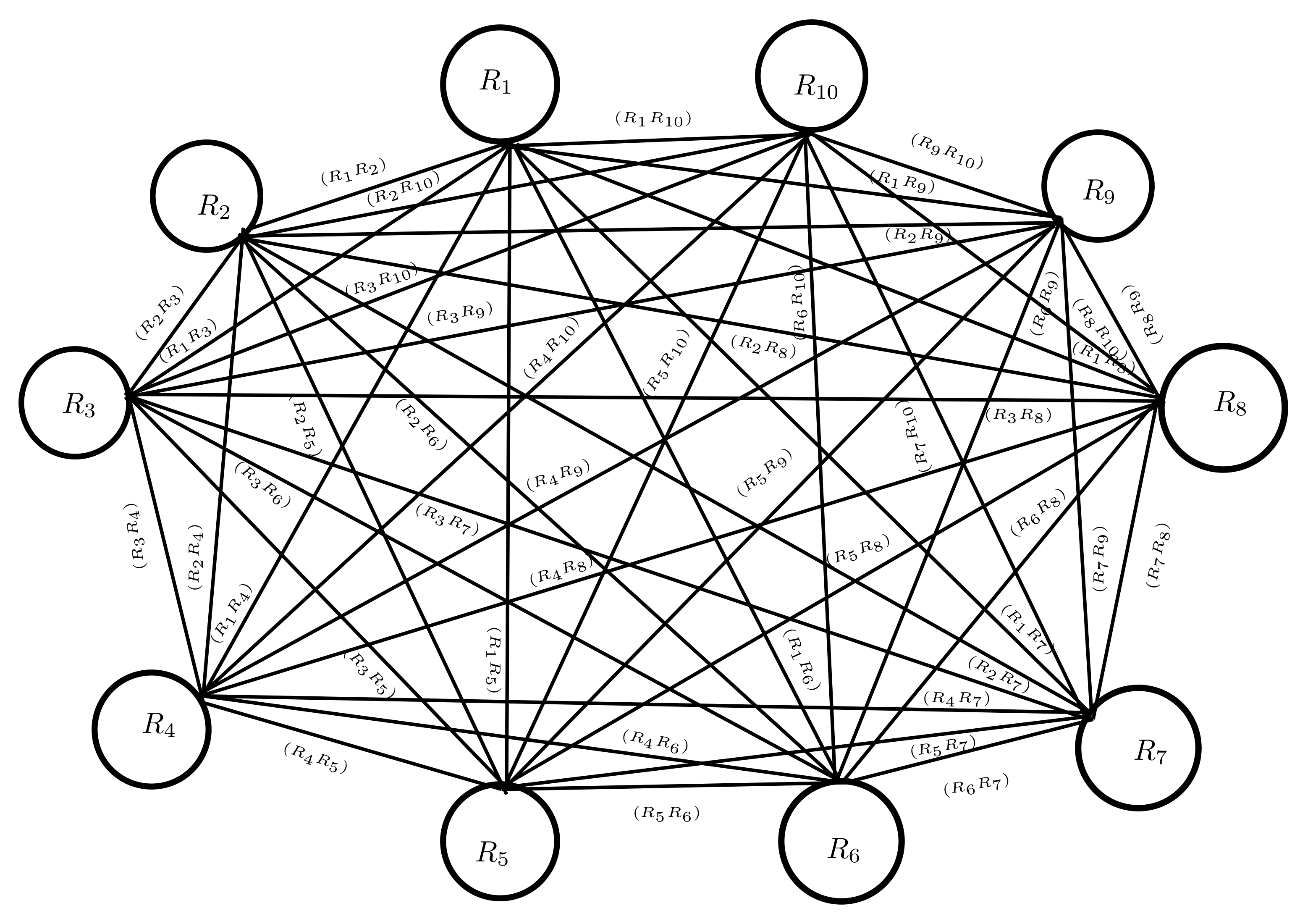
is the largest value and therefore more suitable for making the COVID-19 Designated Tertiary Hospital. CFG with an edge is shown in
Figure 20.


