Compressed-Encoding Particle Swarm Optimization with Fuzzy Learning for Large-Scale Feature Selection

Abstract

Particle swarm optimization (PSO) is a promising method for feature selection. When using PSO to solve the feature selection problem, the probability of each feature being selected and not being selected is the same in the beginning and is optimized during the evolutionary process. That is, the feature selection probability is optimized from symmetry (i.e., 50% vs. 50%) to asymmetry (i.e., some are selected with a higher probability, and some with a lower probability) to help particles obtain the optimal feature subset. However, when dealing with large-scale features, PSO still faces the challenges of a poor search performance and a long running time. In addition, a suitable representation for particles to deal with the discrete binary optimization problem of feature selection is still in great need. This paper proposes a compressed-encoding PSO with fuzzy learning (CEPSO-FL) for the large-scale feature selection problem. It uses the N-base encoding method for the representation of particles and designs a particle update mechanism based on the Hamming distance and a fuzzy learning strategy, which can be performed in the discrete space. It also proposes a local search strategy to dynamically skip some dimensions when updating particles, thus reducing the search space and reducing the running time. The experimental results show that CEPSO-FL performs well for large-scale feature selection problems. The solutions obtained by CEPSO-FL contain small feature subsets and have an excellent performance in classification problems.

1. Introduction

Feature selection is to select an optimal feature subset related to the problem from the whole feature set [1]. It can not only reduce the number of large-scale features and shorten the processing time of data, but also reduces the interference of redundant features on the results [2]. With the rapid development of big data and deep learning technology, the number of features contained in the data have also increased dramatically. Since the number of feature combinations increases exponentially as the number of features increases, feature selection faces the difficulties brought by the massive combination search space and is still a very challenging problem.

There are three main methods of feature selection: the filter method, the wrapper method, and the embedded method [3]. The filter method has a wide range of applications and a high calculation speed but generally achieves a worse performance than the wrapper method in classification problems [4]. The embedded method embeds the feature selection into a specific machine learning training process, so it is more restricted than the wrapper method when used.

Evolutionary computation (EC) techniques have been widely used in solving feature selection problems as one kind of the wrapper methods [5]. Many EC methods have shown their global search capability for the optimal feature subset in the search space [6,7,8,9]. Among the EC techniques, particle swarm optimization (PSO) has the advantage of simple implementation and a fast convergence [10,11,12,13]. Therefore, PSO is a promising EC method to solve feature selection problems [14,15,16,17,18,19,20,21]. When using PSO, the feature selection problem can be treated as a discrete binary optimization problem, whose dimensions represent all the features and the value of each dimension is 1 or 0, indicating that this feature is selected or is not selected, respectively. In the initial swarm of PSO, a feature has a 50% chance of being selected and a 50% chance of being not selected, i.e., the probability distribution of being selected and of not being selected is symmetric. However, in the late stage of PSO, features in the theoretically optimal feature subset should have a higher probability to be selected, i.e., the probability distribution of being selected and being not selected is asymmetric. Therefore, the searching of PSO for the optimal solution is the process of changing the selection probability of each feature from symmetric distribution to asymmetric distribution with the feedback information of the swarm.

There still exist the following problems when using PSO for feature selection. First, in the existing PSO algorithms, a suitable representation and an effective evolution mechanism are still in great need to handle discrete binary optimization problems [22]. Second, when dealing with large-scale features, it is easy for particles to fall into local optima and lead to a poor search performance due to the huge search space, i.e., PSO faces the challenge of “the curse of dimensionality” [5].

Focusing on the challenges faced by PSO in large-scale feature selection problems, this paper proposes a compressed-encoding PSO with fuzzy learning (CEPSO-FL) for efficiently solving the large-scale feature selection problems. The main contributions of this paper can be summarized as follows:

(1)

Proposing a compressed-encoding representation for particles. The compressed-encoding method adopts the N-base encoding instead of the traditional binary encoding for representation. It divides all features into small neighborhoods. The feature selection process then can be performed comprehensively on each neighborhood instead of on every single feature, which provides more information for the search process.

(2)

Developing an update mechanism of velocity and position for particles based on the Hamming distance and a fuzzy learning strategy. The update mechanism has a good explanation in the discrete space, overcoming the difficulty that traditional PSO update mechanisms often work in real-value space but is hard to be explained in discrete space.

(3)

Proposing a local search mechanism based on the compressed-encoding representation for large-scale features. The local search mechanism can skip some dimensions dynamically when updating particles, which decreases the search space and reduces the difficulty of searching for a better solution, so as to reduce running time.

The rest of this paper is organized as follows. In Section 2, the related work of applying PSO to feature selection is introduced. The proposed PSO for large-scale feature selection problems is introduced in detail in Section 3. In Section 4, the experimental results and analysis compared with other state-of-the-art algorithms are given. Finally, the work of this paper is summarized in Section 5.

2. Related Work

In this section, we first give a brief introduction to the basic PSO applied to feature selection. Then, the two main design schemes for applying PSO to feature selection are discussed. Finally, we introduce some representative PSO algorithms for large-scale feature selection.

2.1. Discrete Binary PSO

The feature selection optimization problem is a discrete binary optimization problem. Therefore, the original PSO algorithm [23] proposed for continuous space cannot be used directly to solve feature selection problems. The discrete binary PSO (BPSO) that can be used for feature selection was first proposed by Kennedy and Eberhart [24]. In BPSO, each particle has a position vector and a velocity vector. Each dimension of the position vector can only be 0 or 1, i.e., the value of the position is discrete. However, the value of the velocity is still continuous. For the optimization process in the discrete space, BPSO defines velocity ${\mathit{v}}_{\mathit{i}}$ that can be transformed to indicate the probability of its corresponding position value being one, which is updated during the evolutionary process as

$${\mathit{v}}_{\mathit{i}}={\mathit{v}}_{\mathit{i}}+c_1{r}_1({\mathit{pbest}}_i-{\mathit{x}}_{\mathit{i}})+c_2{r}_2(\mathit{gbest}-{\mathit{x}}_{\mathit{i}}),$$

(1)

where ${\mathit{x}}_{\mathit{i}}$ is the current position of the i-th particle, ${\mathit{pbest}}_{\mathit{i}}$ is the best position found by the particle so far and represents the personal historical experience, $\mathit{gbest}$ is the best position found by all particles and represents the historical experience from other particles, $c_1$ and $c_2$ are acceleration constants and always set to two, $r_1$ and $r_2$ are random values uniformly sampled from (0, 1) independently for each dimension.

Then, BPSO updates the position with Equation (2), where $\mathit{rand}$ is a random value uniformly sampled from (0, 1) and d is the dimension index of the position vector. The Sigmoid function is used to map $v_i^d$ into the (0, 1) interval. If the value of $v_i^d$ is large, then its corresponding position $x_i^d$ is likely to be one.

$$x_i^d=\{\begin{array}{ll}0,\hfill & \mathrm{if} rand>\mathrm{Sigmoid}(v_i^d)\hfill \\ 1,\hfill & \mathrm{otherwise}\hfill \end{array}$$

(2)

2.2. Two Main Design Schemes for Applying PSO to Feature Selection

At present, most discrete PSOs for feature selection are mainly designed in two schemes. In the first design scheme, the PSOs follow the idea of BPSO and define the velocity v as the probability that position x takes a certain discrete value, such as BPSO and bi-velocity discrete PSO (BVDPSO) [25]. Although the value of the position vector is discrete, the value of the velocity vector is continuous and is limited to the interval (0, 1).

The second design scheme is to discretize the existing PSOs. Since feature selection is described as a 0/1 optimization problem, binarizing the continuous value of x can represent the solution to the feature selection problem. Decoding x from continuous space to discrete space usually uses Equation (3):

$$x_i^d=\{\begin{array}{ll}1,\hfill & \mathrm{if} x_i^d>\lambda \hfill \\ 0,\hfill & \mathrm{otherwise}\hfill \end{array},$$

(3)

where $\lambda \in (0, 1)$ is a user-defined threshold and is commonly set to be 0.5. If fewer features are expected in the final solution, the value of $\lambda$ can be set greater than 0.5, otherwise, the value of $\lambda$ can be set less than 0.5. In the search process of the particle swarm, each particle still searches in continuous space, and its values of position and velocity are continuous. Only when evaluating the particle, its position x will be decoded into a discrete value according to the given threshold $\lambda$. It is worth noting that the continuous information is not discarded in discretization and can be utilized in future generations. Most existing PSOs used for feature selection adopt the second design scheme [26,27,28,29].

It is not complicated to convert the continuous PSO into the discrete PSO and it only needs to perform the decoding step on x before evaluating the particles. However, the meanings of the position and velocity in continuous PSOs are different from those in discrete PSOs, which makes the update process of position and velocity hard to be explained. The PSOs implemented by the first design scheme are more reasonable and suitable to solve feature selection problems. However, the performance of the BPSO is usually worse than the PSOs designed by the second scheme [22]. Therefore, how to find a more reasonable design scheme for PSO to handle feature selection problems remains to be solved [5,22].

2.3. PSO for Large-Scale Feature Selection

With the rapid increment of the feature number contained in the data, PSO faces the challenge of the “dimensional curse” when it is used for feature selection. Proposing a new PSO for large-scale feature selection problems has become a new research focus. Gu et al. [27] discretized the competitive swarm optimizer (CSO) that performs well on large-scale continuous optimization problems for the large-scale feature selection problems. Tran et al. [28] proposed the variable-length PSO (VLPSO) to assign different lengths to particles in different subswarms and dynamically change the lengths of particles according to fitness values, which prevented particles from being trapped in local optima for a long time. Song et al. [29] adopted the co-evolution mechanism in PSO and proposed the variable-size cooperative coevolutionary PSO, which divided the feature search space based on the importance of features and adaptively adjusted the sizes of subswarms to search important feature subspaces adequately. Chen et al. [30] proposed an evolutionary multitasking-based PSO algorithm for high-dimensional feature selection problems, which can automatically calculate a suitable threshold for important features and improve the algorithm performance with the variable-range strategy and subset updating mechanism. Since considering the correlation between features and classification labels can provide prior knowledge for feature selection, Song et al. [31] proposed a hybrid feature selection algorithm based on correlation-guided clustering and PSO (HFS-C-P). The HFS-C-P first discards irrelevant features with the filter method, then clusters features based on their correlation values, and finally applies PSO to search for solutions. However, due to the huge search space, many challenges such as premature convergence and huge time consumption remain to be solved when using PSO for feature selection on high-dimension data.

3. Proposed CEPSO-FL Method

In this section, the compressed-encoding representation for particles is first proposed. Then, based on the proposed representation, a discrete update mechanism via a fuzzy learning strategy for particles is designed. Especially for the large-scale feature selection problems, a local search strategy is also proposed. Finally, the overall framework of the proposed CEPSO-FL is given.

3.1. Compressed-Encoding Representation of Particle Position

The traditional representation of the particle position for feature selection problems is to use a binary bit to represent the selection of a feature. Therefore, in an optimization problem with D features, the encoding length of a particle is D. If there are thousands of or more features contained, the encoding length also needs to be thousands or longer, which increases the difficulty of encoding and searching for the optimal solution. To shorten the encoding length of particles, the compressed-encoding representation uses N-base ($N>2$) encoding method and each bit can represent a segment of 0/1 string. The value N should satisfy ${N=2}^n$, where n = 2, 3, 4, and so on.

The process of compressing a 0/1 string with the N-base representation is shown in Figure 1. When N = 8, every three bits under the binary representation are compressed into one 8-base bit. If the original binary bits are not sufficient, the remaining bits will be randomly filled in. During the search process of the swarm, all particles adopt the compressed-encoding representation method. Only when evaluating particles, the N-base representations will be decoded into binary representations to represent solutions to feature selection problems for evaluation. With the compressed-encoding representation, multiple features in the same neighborhood can be selected as a whole. In other words, not only the selection state of the feature itself but also the selection state of the features in its neighborhood can be learned from the representation. Therefore, the information used in the search process for the optimal solution has increased.

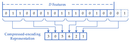
Figure 1. The process of compressing a binary representation into an N-base representation.

3.2. Definitions Based on Compressed-Encoding Representation

Based on the compressed-encoding representation of particle position, the following definitions are given to help design the update mechanism for CEPSO-FL.

3.2.1. Difference between the Positions of Two Particles

The difference $\Delta \left(x_1{, x}_2\right)$ between the positions of two particles p₁ and p₂ is defined as the Hamming distance between their corresponding binary 0/1 strings, as shown in Equation (4), where $x_1$ and $x_2$ are the positions of the two particles, $x^d$ is the value of the d-th dimension of x, function ${\mathrm{h}(x}^d)$ is to get the binary strings represented by $x^d$.

$$x_1^d-x_2^d=\Delta (x_1^d,x_2^d)=\mathrm{Hamming}\mathrm{Distance}(\mathrm{h}(x_1^d),\mathrm{h}(x_2^d))$$

(4)

3.2.2. Velocity of the Particle

The velocity of a particle is defined as the difference between two positions, as shown in Equation (5). Since the value of Hamming distance is discrete, the value of the velocity $v^d$ is also discrete. Hence, $v^d$ can only take the value ${\{0, 1, \dots , \log }_{2}N\}$ under N-base compressed-encoding method.

$$v^d=\Delta (x_1^d,x_2^d)$$

(5)

3.2.3. Addition Operation between the Position and the Velocity

The addition operation between the position value and the velocity value is randomly selecting a position ${\mathit{x}}^{\prime }$ to replace the original position x, as shown in Equation (6), where each dimensional value of the position vector $x^{{}^{\prime }d}$ should satisfy the equation ${\mathrm{Hamming}\mathrm{Distance} \left(\mathrm{h}\right(x}^d{), \mathrm{h}(x}^{{}^{\prime }d}{\left)\right)=v}^d$.

$$x^{{}^{\prime }d}=x^d+v^d$$

(6)

3.3. Update Mechanism with Fuzzy Learning

Based on the above definitions, the velocity of the i-th particle p_i is updated as Equation (7), where w_i is the inertia weight sampled randomly between 0.4 and 0.7, c₁ = c₂ = 1, r₁ and r₂ are a random number between 0 and 1 for each dimension, ${\mathit{cbest}}_{\mathit{i}}$ is the chosen local optimal position for p_i, $\mathit{gbest}$ is the global optimal position obtained by the swarm, and $\left[·\right]$ is the rounding function. In addition, if the value of ${\mathit{v}}_{\mathit{i}}$ is out of range [0, ${\log }_{2}N$], it should be modified to 0 or ${\log }_{2}N$ accordingly.

$${\mathit{v}}_{\mathit{i}}=[w_i{\mathit{v}}_{\mathit{i}}+c_1{r}_1({\mathit{cbest}}_{\mathit{i}}-{\mathit{x}}_{\mathit{i}})+c_2{r}_2(\mathit{gbest}-{\mathit{x}}_{\mathit{i}})]$$

(7)

The traditional update mechanism of the position vector can only rely on the velocity vector because the result of adding two real numbers is unique. However, based on the above definitions, the result of adding the same $x$ and the same $v$ in the discrete space is uncertain. In other words, depending on the value of velocity to update the position vector is not appropriate when using the compressed-encoding representation. Therefore, each particle p_i updates its position $x^d$ with Equation (8). In most cases, the particle jumps directly to ${\mathit{cbest}}_{\mathit{i}}$, which can speed up the convergence rate. In the rest of the cases, the particle moves in the direction of the learned optimal position that is subject to the ${\mathit{cbest}}_{\mathit{i}}$ and the gbest and can increase the diversity of direction to help the particle search in a more promising space.

$$x_{i }^d=\{\begin{array}{ll}{x}_i^d+v_i^d,\hfill & \mathrm{if} rand<0.1\hfill \\ cbes{t}_i^d,\hfill & \mathrm{otherwise}\hfill \end{array}$$

(8)

In the proposed update mechanism, the update of position relies more on the ${\mathit{cbest}}_{\mathit{i}}$, so the choice of ${\mathit{cbest}}_{\mathit{i}}$ is critical. To increase the diversity of learning sources, the ${\mathit{cbest}}_{\mathit{i}}$ chosen by p_i can be the $\mathit{pbest}$ of itself, the $\mathit{pbest}$ of another particle, or the $\mathit{pbest}$ that has been eliminated.

Here, a fuzzy learning strategy is adopted to help make the decision. First, factor $F$ is introduced to evaluate the performance of the current position of a particle, which can be calculated by

$$F=\frac{cur\_fitness}{pbest\_fitness},$$

(9)

where $\mathit{cur}\_\mathit{fitness}$ is the fitness of the current position and $\mathit{pbest}\_\mathit{fitness}$ is the fitness of the historical optimal position. The feature selection for classification is a maximization optimization problem because the classification accuracy is adopted as the fitness of a solution. Therefore, a small value of $F$ means that the particle is in a bad position so it can choose its historical optimal position for learning. However, a large value of $F$ means that the current position has a similar performance to the historical optimal position and the particle is difficult to improve itself by continuing to choose its personal optimal position for learning. Turning to other local optimal positions for learning is a better choice when the value of $F$ is large. Therefore, according to the value of $F$, the membership grade for the three search states of a particle is defined in Figure 2.

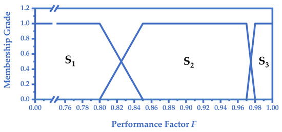
Figure 2. Fuzzy membership functions for the three search states of a particle.

The design philosophy of the fuzzy membership functions is to guide the particle to learn from itself when it performs well and learns from other particles when it performs poorly and needs to be improved. In the first state $S_1$, the value of $F$ is small, so the particle p_i chooses its $\mathit{pbest}$ as ${\mathit{cbest}}_i$. The fuzzy membership function $\mu$ of $S_1$ is defined as

$${\mu }_{S_1}(F)=\{\begin{array}{ll}1,\hfill & 0\le F<0.80\hfill \\ -20\times F+17,\hfill & 0.80\le F<0.85\hfill \\ 0,\hfill & 0.85\le F\le 1\hfill \end{array}.$$

(10)

In the second state $S_2$, the value of $F$ becomes larger, and the learning scope of p_i is extended to the whole swarm. It randomly chooses two particles from the swarm and selects the $\mathit{pbest}$ that performs better from the two particles as ${\mathit{cbest}}_{\mathit{i}}$. Since p_i is not excluded from the random selection, it is still possible that p_i uses its $\mathit{pbest}$ as ${\mathit{cbest}}_{\mathit{i}}$. The fuzzy membership function $\mu$ of $S_2$ is defined as

$${\mu }_{S_2}(F)=\{\begin{array}{ll}0,\hfill & 0\le F<0.80\hfill \\ 20\times F-16,\hfill & 0.80\le F<0.85\hfill \\ 1,\hfill & 0.85\le F<0.97\hfill \\ -100\times F+98,\hfill & 0.97\le F<0.98\hfill \\ 0,\hfill & 0.98\le F\le 1\hfill \end{array}.$$

(11)

In the third state $S_3$, the value of $F$ is very close to 1, which means that the particle is at, or very close to, the historical optimal position. To make full use of the historical information, all the eliminated $\mathit{pbest}$ are stored in an archive. Note that the archive is set as empty in the beginning and when any particle updates its $\mathit{pbest}$ with its current position, the $\mathit{pbest}$ is stored into the archive. Moreover, the archive has a size limitation, so that when a new $\mathit{pbest}$ comes, a random $\mathit{pbest}$ in the archive is removed. Then particles in the state $S_3$ randomly pick one position from the archive as their ${\mathit{cbest}}_{\mathit{i}}$. The fuzzy membership function $\mu$ of $S_3$ can be described as

$${\mu }_{S_3}(F)=\{\begin{array}{ll}0,\hfill & 0\le F<0.97\hfill \\ 100\times F-97,\hfill & 0.97\le F<0.98\hfill \\ 1,\hfill & 0.98\le F\le 1\hfill \end{array}.$$

(12)

After calculating the membership functions of the three states, if the membership grade of F is 1 it belongs to only one state, then p_i chooses this state as its current state. However, there exists a special case since the fuzzy logic of the state transition sequence is $S_1\Rightarrow S_2\Rightarrow S_3$. If a particle is in a transition zone between two states (i.e., the membership grade of both states is not 0) and the state that comes first in the sequence $S_1\Rightarrow S_2\Rightarrow S_3$ is the same as its previous state, the particle will keep its previous state unchanged to maintain logical stability. For example, if a particle is in the transition zone between $S_1$ and $S_2$, and its previous state is $S_1$, then it will remain in $S_1$. Otherwise, it will shift to $S_1$ or $S_2$ according to the value of $F$.

3.4. Local Search Strategy

For large-scale feature selection problems, a local search strategy based on the compressed-encoding representation is proposed to reduce the search space and improve computational efficiency. The process of the local search strategy is described in Algorithm 1. The value of the position $x_i^d$ updates only when its corresponding ${\mathit{pbest}}_i^d$ is not zero. Otherwise, the value of $x_i^d$ is set to 0, which is the same as the ${\mathit{pbest}}_i^d$.

Algorithm 1: Local Search Strategy

Input: The position xi of particle pi, the encoding length D′ after compression, the index of the particle i. Output: The $x_i$ updated by the local search strategy. begin   $\mathbf{for} d=1 to D^{\prime } \mathbf{do}$     $\mathbf{if} ({\mathit{pbest}}_i^d \ne 0) \mathbf{then}$       $\mathrm{Update} x_i^d \mathrm{with} \mathrm{Equation} \left(8\right);$     else       $x_i^d \leftarrow 0;$     end   end   $\mathbf{return} x_i;$ end

With the local search strategy, some bits of the position are dynamically set to 0 and no longer updated, as shown in Figure 3. In the process of searching for an optimal solution, each particle p_i only handles the features represented by the bits whose values are not set to 0 in the ${\mathit{pbest}}_i$ instead of all features. Thus, the actual length of the position is shortened and the search space for the particle is reduced. In addition, since the ignored bits in different particles are different, each particle can search in different feature subsets and the diversity of the swarm is retained.

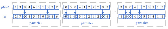
Figure 3. Local search strategy when N = 8.

The particle may miss the global optimal solution because parts of the search space are discarded by the local search strategy. However, under the N-base compressed-encoding representation, a value of 0 in ${\mathit{pbest}}_{\mathit{i}}$ means that all features in the same neighborhood represented by ${\mathit{pbest}}_i^d$ are not selected at the same time. Therefore, the probability of skipping a bit of $x_i$ is reduced to $1/N$, which reduces the probability of blindly reducing the search space by the local search strategy.

3.5. Overall Framework

The overall framework of the proposed CEPSO-FL is described in Algorithm 2. Before the initialization, the value of symmetric uncertainty (SU) between each feature and the classification label is obtained and all features are sorted in descending order according to the SU values. SU is an information measure to describe the symmetry correlation relationship between features and labels and can be used as a filter method for feature selection [32]. After the feature sorting, each feature and the features near it, i.e., features in the neighborhood, have a similar effect on the classification result, which is conducive to the search process because CEPSO-FL also uses the information from the neighborhood for searching. Then, the length of particle representation $D^{\prime }$ after compression can be calculated according to the number of features D and the given N. To reduce the cost of computing the Hamming distance, an $N \times N$ table is constructed in advance, which stores the Hamming distance between any two binary strings represented by the N-base numbers.

Algorithm 2: CEPSO-FL

Input: The maximum number of fitness evaluations $\mathit{MAX}\_\mathit{FE}$, the size of the swarm $P$, the number of the features $D$, the base for encoding compression $N$. Output: The global optimal position $\mathit{gbest}$. begin   Calculate the SU value between each feature and label;   Sort features according to the SU values;   D’ ← ⎡D/log2N⎤;   Construct the N × N Hamming distance table;   $\mathit{FE} \leftarrow 0$;   Randomly initialize $\mathit{x}$ and $\mathit{v}$ of each particle;   for $i = 1$ to $P$ do     Decode and evaluate ${\mathit{x}}_{\mathit{i}}$;     Update ${\mathit{pbest}}_{\mathit{i}}$;     $\mathit{FE} \leftarrow \mathit{FE} + 1$   end   Update $\mathit{gbest}$;   while $\mathit{FE} < \mathit{MAX}\_\mathit{FE}$ do     for $i = 1$ to $P$ do       Update vi with Equation (7);       Update xi with Algorithm 1;     end     for $i = 1$ to $P$ do       Decode and evaluate ${\mathit{x}}_{\mathit{i}}$;       Update ${\mathit{pbest}}_{\mathit{i}}$;       $\mathit{FE} \leftarrow \mathit{FE} + 1$     end     Update $\mathit{gbest}$;   end   return $\mathit{gbest}$ end

Before evaluation, the particle needs to be decoded into a binary string to represent a solution of feature selection, in which the value 1 means that the corresponding feature is selected and the value 0 means that it is not selected. Then, the process of particles being updated and evaluated repeats until the terminal conditions are met.

In the worst case, the time complexity of CEPSO-FL is $\mathrm{O}(\mathit{MAX}\_\mathit{FE} \times \mathit{P} \times \mathit{D})$. However, because CEPSO-FL uses the local search strategy to shorten the encoding length, the actual time consumption of CEPSO-FL is always less than that of the traditional PSOs, as shown in Section 4.

In addition, although CEPSO-FL is proposed for large-scale feature selection problems, it can also solve other binary discrete optimization problems by simply removing the local search strategy and the feature sorting step designed especially for feature selection.

4. Experiments and Analysis

In this section, experiments for CEPSO-FL and other PSO-based feature selection algorithms on data containing large-scale features are carried out to verify the effectiveness of the proposed CEPSO-FL.

4.1. Datasets

The experiments use 12 open-access classification datasets for feature selection, which can be downloaded from https://ckzixf.github.io/dataset.html, accessed on 11 April 2022, [30] and https://jundongl.github.io/scikit-feature/datasets.html, accessed on 11 April 2022, [33]. Table 1 lists the detailed information of the 12 datasets. All the considered datasets contain large-scale features but many of them only have small samples. Besides, the distribution of some used datasets is unbalanced such as Leukemia_2 and GLIOMA.

Table 1. Detailed information of 12 datasets.

Index	Dataset	Samples	Features	Categories
1	Madelon	500	500	2
2	Isolet	500	617	26
3	COIL20	500	1024	20
4	Yale	165	1024	15
5	ORL	400	1024	40
6	WarpAR10P	130	2400	10
7	Lung	203	3312	5
8	Lymphoma	96	4026	9
9	GLIOMA	50	4434	4
10	Brain_Tumor_1	90	5920	5
11	Prostate_GE	102	5966	2
12	Leukemia_2	72	7129	4

4.2. Algorithms for Comparison and Parameter Settings

There are six PSO-based feature selection algorithms for comparison with CEPSO-FL. The parameter settings of each algorithm are listed in Table 2. BPSO, BBPSO-ACJ, BVDPSO, and CSO are all discrete binary PSOs that are suitable for solving feature selection problems. However, they are not optimized especially for large-scale features. VLPSO and HFS-C-P are algorithms proposed for large-scale feature selection. They both use correlation measurement methods such as SU to analyze features.

Table 2. Parameter settings of algorithms.

Algorithm	Parameter Settings
BPSO [24]	P = 20, the range of velocity: [−6, 6], c1 = c2 = 2.01, w = 1.
BVDPSO [25]	P = 20, the range of w: [0.4, 0.9], c1 = c2 = 2, selected threshold α = 0.5.
BBPSO-ACJ [26]	P = 20, chaotic factor z0 = 0.13, selected threshold λ = 0.5.
CSO [27]	P = 100, control factor ϕ = 0.1, selected threshold λ = 0.5.
VLPSO [28]	P = min{features/20,300}, c = 1.49445, the range of w: [0.4, 0.9], selected threshold λ = 0.6, max iterations to renew exemplar: 7, number of divisions: 12, max iterations for length changing: 9.
HFS-C-P [31]	P = 20.
CEPSO-FL	P = 20, archive size: 100, c1 = c2 = 1, the range of w: [0.4, 0.7], N = 8.

The maximum number of fitness evaluations is set to 5000 for all algorithms. On each dataset, the 10-fold cross-validation method is used to divide samples into a feature selection dataset and a test dataset. The whole feature selection dataset is used as the training dataset when testing the selected features on the test dataset. Then, each algorithm runs 10 times on 10 groups of feature selection data and test data and adopts the average results as the final results. In the feature selection phase, particles use the leave-one-out cross-validation method on the feature selection dataset to obtain fitness values for evaluation. The k-nearest neighbor (k-NN) method is chosen as the classifier to calculate the classification accuracy values of the selected features in the experiments and k is set to be five. When the accuracy values are the same, the particle with fewer features is regarded to perform better.

In addition, the Wilcoxon signed-rank test is employed to verify a significant difference between CEPSO-FL and other compared algorithms, with a significance level of $\alpha =0.05$. In the experimental statistical results, symbol “+” indicates that CEPSO-FL is significantly superior to the compared algorithm, symbol “−” indicates that CEPSO-FL is significantly inferior to the compared algorithm, and symbol “=” indicates that there is no significant difference between CEPSO-FL and the compared algorithm at the current significant level. All algorithms are implemented in C++ and are run on a PC with an Intel Core i7-10700F CPU @ 2.90GHz and a total memory of 8 GB.

4.3. Experimental Results and Discussion

The average classification accuracy values on the test dataset (Test Acc) of each algorithm on 12 datasets are shown in Table 3. The Test Acc of CEPSO-FL performs better than BPSO, BVDPSO, and CSO, with a significant advantage on two datasets and a disadvantage on one dataset, respectively. CEPSO-FL also performs better than HFS-C-P with a higher Test Acc on the dataset Lung and a similar Test Acc on other datasets. Compared with BBPSO-ACJ and VLPSO, CEPSO-FL has a similar Test Acc performance. On most datasets, there is no significant difference between the Test Acc of CEPSO-FL and the Test Acc of other algorithms.

Table 3. The Test Acc of algorithms on the 12 datasets.

Data	BPSO	BVDPSO	CSO	BBPSO-ACJ	VLPSO	HFS-C-P	CEPSO-FL
Madelon	0.690(+)	0.694(+)	0.720(+)	0.706(+)	0.720(+)	0.748(=)	0.780
Isolet	0.878(−)	0.882(−)	0.874(−)	0.890(−)	0.878(−)	0.828(=)	0.834
COIL20	0.906(=)	0.914(=)	0.910(=)	0.922(−)	0.890(=)	0.898(=)	0.892
Yale	0.535(=)	0.541(=)	0.535(=)	0.541(=)	0.518(=)	0.547(=)	0.582
ORL	0.903(=)	0.883(=)	0.900(=)	0.898(=)	0.873(=)	0.903(=)	0.878
WarpAR10P	0.531(+)	0.538(+)	0.600(=)	0.600(=)	0.569(=)	0.654(=)	0.669
Lung	0.914(=)	0.919(=)	0.910(=)	0.919(=)	0.895(=)	0.867(+)	0.910
Lymphoma	0.810(=)	0.810(=)	0.800(=)	0.830(=)	0.820(=)	0.810(=)	0.790
GLIOMA	0.760(=)	0.800(=)	0.740(=)	0.800(=)	0.740(=)	0.700(=)	0.740
Brain_Tumor_1	0.856(=)	0.822(=)	0.844(=)	0.844(=)	0.856(=)	0.867(=)	0.822
Prostate_GE	0.773(=)	0.782(=)	0.755(+)	0.736(+)	0.764(=)	0.818(=)	0.809
Leukemia_2	0.750(=)	0.750(=)	0.750(=)	0.738(=)	0.738(=)	0.763(=)	0.775
+/=/−	2/9/1	2/9/1	2/9/1	2/8/2	1/10/1	1/11/0	NA

The bold represents the best value among all algorithms.

However, in terms of the average number of features included in the found optimal solution (Feature Num), CEPSO-FL is significantly smaller than other algorithms on most datasets. The experimental results are shown in Table 4. The Feature Num of CEPSO-FL is smaller than the Feature Num of BPSO, BVDPSO, CSO, and BBPSO-ACJ on all datasets and is smaller than the Feature Num of VLPSO on 11 datasets. On datasets Lung, GLIOMA, and Prostate_GE, the Feature Num of CEPSO-FL is larger than HFS-C-P but still smaller than other algorithms. On other datasets, CEPSO-FL can obtain a smaller Feature Num than HFS-C-P. HFS-C-P is a three-phase algorithm, its Feature Num depends on correlation-guided clustering results given by the first two stages. Therefore, the Feature Num performance of HFS-C-P can vary greatly on different datasets. For example, on datasets Lung, GLIOMA, and Prostate_GE, HFS-C-P can find the smallest feature subset. However, on datasets Yale and ORL, the Feature Num obtained by HFS-C-P is larger than most of the compared algorithms. In contrast, CEPSO-FL always finds a small feature subset on different datasets.

Table 4. The Feature Num of algorithms on the 12 datasets.

Data	BPSO	BVDPSO	CSO	BBPSO-ACJ	VLPSO	HFS-C-P	CEPSO-FL
Madelon	309.5(+)	321.8(+)	157.9(+)	197.8(+)	87.8(+)	83.8(+)	8.3
Isolet	377.2(+)	385.8(+)	356.7(+)	273.0(+)	187.5(+)	238.2(+)	78.3
COIL20	620.3(+)	595.5(+)	260.8(+)	288.1(+)	287.8(+)	394.4(+)	78.7
Yale	626.5(+)	602.9(+)	412.5(+)	376.7(+)	330.4(+)	625.4(+)	90.2
ORL	629.4(+)	649.9(+)	713.2(+)	505.5(+)	390.0(+)	874.2(+)	100.6
WarpAR10P	1485.2(+)	1431.4(+)	442.1(+)	126.1(+)	478.8(+)	565.9(+)	19.5
Lung	2048.7(+)	1829.0(+)	1401.4(+)	1086.1(+)	743.1(=)	19.1(−)	373.8
Lymphoma	2356.7(+)	2219.4(+)	1402.8(+)	1382.1(+)	1135.5(+)	508.9(+)	187.5
GLIOMA	2611.1(+)	2402.5(+)	1566.6(+)	1932.5(+)	389.1(+)	9.5(−)	86.1
Brain_Tumor_1	3547.0(+)	3403.1(+)	3009.3(+)	1348.6(+)	1375.8(+)	1452.8(+)	191.2
Prostate_GE	3667.2(+)	3392.2(+)	2186.7(+)	1043.9(+)	1474.4(+)	12.1(−)	63.0
Leukemia_2	4399.9(+)	4234.6(+)	3219.4(+)	2523.4(+)	2150.6(+)	607.0(+)	221.7
+/=/−	12/0/0	12/0/0	12/0/0	12/0/0	11/1/0	9/0/3	NA

The bold represents the best value among all algorithms.

The running time for each algorithm on the 12 datasets (Time) is listed in Table 5. The Time of CEPSO-FL is less than algorithms that are not proposed especially for the large-scale features, i.e., BPSO, CSO, BVDPSO, and BBPSO-ACJ on most datasets. CEPSO-FL also performs better than the three-phase HFS-C-P on nine datasets. CEPSO-FL can reduce the search time for two reasons. One reason is that the local search strategy can skip the calculation of some dimensions when updating particles. Another reason is that the adopted k-NN classifier needs to calculate the Euclidean distance of two samples for evaluation. The fewer the features they contain, the less time the calculation will spend. Because the local search strategy can lead particles to search for solutions with fewer features, the running time of CEPSO-FL is less than other algorithms except for VLPSO. Though CEPSO-FL spends more time searching than VLPSO on eight datasets, it can achieve a better Test Acc and Feature Num on most datasets.

Table 5. The Time (min) of algorithms.

Data	BPSO	BVDPSO	CSO	BBPSO-ACJ	VLPSO	HFS-C-P	CEPSO-FL
Madelon	64.4	64.5	62.9	50.9	26.6	53.5	52.2
Isolet	78.7	79.9	145.9	65.6	40.1	148.1	72.7
COIL20	136.8	127.9	143.0	112.1	51.9	178.2	112.6
Yale	15.2	14.7	16.2	12.1	7.2	23.6	13.2
ORL	83.8	87.3	102.5	73.4	47.8	195.8	80.0
WarpAR10P	39.0	57.7	29.8	27.6	10.4	23.3	15.8
Lung	210.3	183.2	160.6	104.9	51.2	50.1	61.7
Lymphoma	65.0	62.6	50.4	36.8	13.9	33.3	16.2
GLIOMA	20.1	20.5	15.4	11.2	6.1	4.0	4.2
Brain_Tumor_1	84.6	96.4	66.8	51.9	28.6	66.8	19.4
Prostate_GE	113.4	113.5	88.5	64.9	37.8	21.7	24.1
Leukemia_2	70.9	68.1	44.7	38.8	28.5	28.9	16.1

The bold represents the best value among all algorithms.

The average classification accuracy value on the feature selection dataset (Train Acc) can show the learning ability of each algorithm on different datasets. Therefore, the Train Acc of each algorithm after each evaluation on all datasets is plotted in Figure 4 to further analyze the performance of the algorithms. The proposed CEPSO-FL performs well and achieves a high Train Acc on most datasets. On datasets Isolet, COIL20, and ORL, the Train Acc of CEPSO-FL is lower than the Train Acc of CSO and BVDPSO. However, on datasets with more features, CEPSO-FL is superior to CSO and BVDPSO on Train Acc. On datasets Brain_Tumor_1, Prostate_GE, and Leukemia_2, CEPSO-FL obtains a lower Train Acc than HFS-C-P but is still superior to other algorithms for comparison, while on datasets with fewer features, CEPSO-FL has a better performance than HFS-C-P. In general, CEPSO-FL has a better learning ability for different datasets compared to other algorithms, so it can adapt to datasets with different feature numbers.

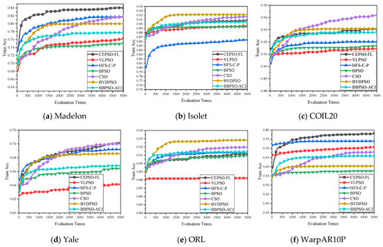
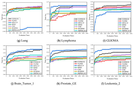
Figure 4. The Train Acc of algorithms on 12 datasets with the increasement of evaluation times. (a–l) shows the Train Acc from evaluation times 0 to 5000 on dataset Madelon, Isolet, COIL20, Yale, ORL, WarpAR10P, Lung, Lymphoma, GLIOMA, Brain_Tumor_1, Prostate_GE, and Leukemia_2, respectively.

The effects of the parameter N are also studied because N determines the compression ratio of the representation. If N is large, the compressed representation of the particle is much shorter, and the probability of features being skipped when applying the local search strategy is much smaller than that with a small N. Since N needs to be an integer power of two, the value of N is set to be 2 ($2^1$), 8 ($2^3$), and 32 ($2^5$), and the comparison results are listed in Table 6. In general, when the value of N increases, the feature subset obtained by CEPSO-FL has a higher Test Acc but contains more features and needs more time for searching. CEPSO-FL with N = 8 can achieve a higher Test Acc than that with N = 2 on all datasets. In some cases, the Test Acc consistently improves when the value of N increases. For example, on datasets Madelon, Isolet, COIL20, WarpAR10P, and Lymphoma, CEPSO-FL can get the highest Test Acc with N = 32. However, sometimes the Test Acc decreases when the value of N becomes larger, e.g., on datasets Yale, ORL, Lung, and Prostate_GE. Therefore, it is recommended that N be set to eight in most cases, but a larger N can be tried to further improve the value of Test Acc.

Table 6. Comparison among CEPSO-FL with different N.

Data	Test Acc			Feature Num			Time (min)
	N = 2	N = 8	N = 32	N = 2	N = 8	N = 32	N = 2	N = 8	N = 32
Madelon	0.788	0.780	0.802	7.7	8.3	19.6	49.8	52.2	70.6
Isolet	0.838	0.834	0.844	90.6	78.3	67.4	70.9	72.7	75.4
COIL20	0.874	0.892	0.902	45.0	78.7	75.2	111.5	112.6	114.3
Yale	0.547	0.582	0.535	99.4	90.2	127.0	14.0	13.2	13.4
ORL	0.868	0.878	0.838	115.6	100.6	100.4	81.6	80.0	76.5
WarpAR10P	0.592	0.669	0.692	22.9	19.5	43.7	15.7	15.8	16.3
Lung	0.895	0.910	0.895	359.7	373.8	286.7	57.8	61.7	69.3
Lymphoma	0.790	0.790	0.840	266.4	187.5	349.6	16.1	16.2	16.3
GLIOMA	0.680	0.740	0.700	136.2	86.1	74.8	4.6	4.2	4.6
Brain_Tumor_1	0.778	0.822	0.822	204.4	191.2	145.6	19.7	19.4	20.5
Prostate_GE	0.782	0.809	0.800	17.7	63.0	99.7	23.9	24.1	26.0
Leukemia_2	0.713	0.775	0.775	219.9	221.7	305.3	15.9	16.1	15.7
Rank Sum	31	19	20	24	23	25	20	22	30

The bold represents the best value among all the CEPSO-FL variants with different N.

5. Conclusions

This paper proposes a discrete PSO algorithm named CEPSO-FL for large-scale feature selection problems. CEPSO-FL adopts the N-base encoding method and treats the features compressed in the same neighborhood as a whole for selection. Then, CEPSO-FL designs the update mechanism for particles based on the Hamming distance and the fuzzy learning strategy, which has a logical explanation in the discrete space. For the large-scale features, CEPSO-FL proposes a local search strategy to help particles search in a smaller feature space and improve computational efficiency. Experimental results show that CEPSO-FL is promising in large-scale feature selection. It can always select a feature subset that contains a small number of features but performs well on classification problems. The running time of CEPSO-FL is also less than most compared algorithms.

For future work, some promising methods can be tried to reduce the computational cost of evaluations [34,35] and further improve the performance of the proposed algorithm on more complex feature selection problems [36].

References

- Dash, M. Feature Selection via set cover. In Proceedings of the Proceedings 1997 IEEE Knowledge and Data Engineering Exchange Workshop, Newport Beach, CA, USA, 4 November 1997; pp. 165–171. [Google Scholar]
- Ladha, L.; Deepa, T. Feature selection methods and algorithms. Int. J. Comput. Sci. Eng. 2011, 3, 1787–1797. [Google Scholar]
- Chandrashekar, G.; Sahin, F. A survey on feature selection methods. Comput. Electr. Eng. 2014, 40, 16–28. [Google Scholar] [CrossRef]
- Khalid, S.; Khalil, T.; Nasreen, S. A survey of feature selection and feature extraction techniques in machine learning. In Proceedings of the 2014 Science and Information Conference, London, UK, 27–29 August 2014; pp. 372–378. [Google Scholar]
- Xue, B.; Zhang, M.; Browne, W.N.; Yao, X. A Survey on Evolutionary Computation Approaches to Feature Selection. IEEE Trans. Evol. Comput. 2016, 20, 606–626. [Google Scholar] [CrossRef] [Green Version]
- Oreski, S.; Oreski, G. Genetic algorithm-based heuristic for feature selection in credit risk assessment. Expert Syst. Appl. 2014, 41, 2052–2064. [Google Scholar] [CrossRef]
- Mistry, K.; Zhang, L.; Neoh, S.C.; Lim, C.P.; Fielding, B. A micro-GA embedded PSO feature selection approach to intelligent facial emotion recognition. IEEE Trans. Cybern. 2017, 47, 1496–1509. [Google Scholar] [CrossRef] [Green Version]
- Zhang, Y.; Gong, D.; Gao, X.; Tian, T.; Sun, X. Binary differential evolution with self-learning for multi-objective feature selection. Inf. Sci. 2020, 507, 67–85. [Google Scholar] [CrossRef]
- Xu, H.; Xue, B.; Zhang, M. A duplication analysis-based evolutionary algorithm for biobjective feature selection. IEEE Trans. Evol. Comput. 2021, 25, 205–218. [Google Scholar] [CrossRef]
- Liu, X.F.; Zhan, Z.H.; Gao, Y.; Zhang, J.; Kwong, S.; Zhang, J. Coevolutionary particle swarm optimization with bottleneck objective learning strategy for many-objective optimization. IEEE Trans. Evol. Comput. 2019, 23, 587–602. [Google Scholar] [CrossRef]
- Wang, Z.J.; Zhan, Z.H.; Kwong, S.; Jin, H.; Zhang, J. Adaptive granularity learning distributed particle swarm optimization for large-scale optimization. IEEE Trans. Cybern. 2021, 51, 1175–1188. [Google Scholar] [CrossRef]
- Jian, J.R.; Chen, Z.G.; Zhan, Z.H.; Zhang, J. Region encoding helps evolutionary computation evolve faster: A new solution encoding scheme in particle swarm for large-scale optimization. IEEE Trans. Evol. Comput. 2021, 25, 779–793. [Google Scholar] [CrossRef]
- Li, J.Y.; Zhan, Z.H.; Liu, R.D.; Wang, C.; Kwong, S.; Zhang, J. Generation-level parallelism for evolutionary computation: A pipeline-based parallel particle swarm optimization. IEEE Trans. Cybern. 2021, 51, 4848–4859. [Google Scholar] [CrossRef] [PubMed]
- Tran, B.; Xue, B.; Zhang, M. Improved PSO for feature selection on high-dimensional datasets. In Lecture Notes in Computer Science, Proceedings of the Simulated Evolution and Learning, Dunedin, New Zealand, 2014; Dick, G., Browne, W.N., Whigham, P., Zhang, M., Bui, L.T., Ishibuchi, H., Jin, Y., Li, X., Shi, Y., Singh, P., et al., Eds.; Springer International Publishing: Cham, Switzerland, 2014; pp. 503–515. [Google Scholar]
- Zhang, Y.; Gong, D.; Sun, X.; Geng, N. Adaptive bare-bones particle swarm optimization algorithm and its convergence analysis. Soft Comput. 2014, 18, 1337–1352. [Google Scholar] [CrossRef]
- Abualigah, L.M.; Khader, A.T.; Hanandeh, E.S. A new feature selection method to improve the document clustering using particle swarm optimization algorithm. J. Comput. Sci. 2018, 25, 456–466. [Google Scholar] [CrossRef]
- Wang, Y.Y.; Zhang, H.; Qiu, C.H.; Xia, S.R. A novel feature selection method based on extreme learning machine and fractional-order darwinian PSO. Comput. Intell. Neurosci. 2018, 2018, e5078268. [Google Scholar] [CrossRef]
- Bhattacharya, A.; Goswami, R.T.; Mukherjee, K. A feature selection technique based on rough set and improvised PSO algorithm (PSORS-FS) for permission based detection of android malwares. Int. J. Mach. Learn. Cyber. 2019, 10, 1893–1907. [Google Scholar] [CrossRef]
- Huda, R.K.; Banka, H. Efficient feature selection and classification algorithm based on PSO and rough sets. Neural Comput. Applic. 2019, 31, 4287–4303. [Google Scholar] [CrossRef]
- Huda, R.K.; Banka, H. New efficient initialization and updating mechanisms in PSO for feature selection and classification. Neural Comput. Applic. 2020, 32, 3283–3294. [Google Scholar] [CrossRef]
- Zhou, Y.; Lin, J.; Guo, H. Feature subset selection via an improved discretization-based particle swarm optimization. Appl. Soft Comput. 2021, 98, 106794. [Google Scholar] [CrossRef]
- Nguyen, B.H.; Xue, B.; Zhang, M. A survey on swarm intelligence approaches to feature selection in data mining. Swarm Evol. Comput. 2020, 54, 100663. [Google Scholar] [CrossRef]
- Kennedy, J.; Eberhart, R. Particle swarm optimization. In Proceedings of the ICNN’95—International Conference on Neural Networks, Perth, Australia, 27 November–1 December 1995; Volume 4, pp. 1942–1948. [Google Scholar]
- Kennedy, J.; Eberhart, R.C. A discrete binary version of the particle swarm algorithm. In Proceedings of the Computational Cybernetics and Simulation 1997 IEEE International Conference on Systems, Man, and Cybernetics, Orlando, EL, USA, 12–15 October 1997; Volume 5, pp. 4104–4108. [Google Scholar]
- Shen, M.; Zhan, Z.H.; Chen, W.; Gong, Y.; Zhang, J.; Li, Y. Bi-Velocity discrete particle swarm optimization and its application to multicast routing problem in communication networks. IEEE Trans. Ind. Electron. 2014, 61, 7141–7151. [Google Scholar] [CrossRef]
- Qiu, C. Bare bones particle swarm optimization with adaptive chaotic jump for feature selection in classification. Int. J. Comput. Intell. Syst. 2018, 11, 1. [Google Scholar] [CrossRef] [Green Version]
- Gu, S.; Cheng, R.; Jin, Y. Feature selection for high-dimensional classification using a competitive swarm optimizer. Soft Comput. 2018, 22, 811–822. [Google Scholar] [CrossRef] [Green Version]
- Tran, B.; Xue, B.; Zhang, M. Variable-length particle swarm optimization for feature selection on high-dimensional classification. IEEE Trans. Evol. Comput. 2019, 23, 473–487. [Google Scholar] [CrossRef]
- Song, X.F.; Zhang, Y.; Guo, Y.N.; Sun, X.Y.; Wang, Y.L. Variable-size cooperative coevolutionary particle swarm optimization for feature selection on high-dimensional data. IEEE Trans. Evol. Comput. 2020, 24, 882–895. [Google Scholar] [CrossRef]
- Chen, K.; Xue, B.; Zhang, M.; Zhou, F. An evolutionary multitasking-based feature selection method for high-dimensional classification. IEEE Trans. Cybern. 2020, in press. [Google Scholar] [CrossRef]
- Song, X.F.; Zhang, Y.; Gong, D.W.; Gao, X.Z. A fast hybrid feature selection based on correlation-guided clustering and particle swarm optimization for high-dimensional data. IEEE Trans. Cybern. 2021, in press. [Google Scholar] [CrossRef] [PubMed]
- Bommert, A.; Sun, X.; Bischl, B.; Rahnenführer, J.; Lang, M. Benchmark for filter methods for feature selection in high-dimensional classification data. Comput. Stat. Data Anal. 2020, 143, 106839. [Google Scholar] [CrossRef]
- Li, J.; Cheng, K.; Wang, S.; Morstatter, F.; Trevino, R.P.; Tang, J.; Liu, H. Feature selection: A data perspective. ACM Comput. Surv. 2017, 50, 94:1–94:45. [Google Scholar] [CrossRef] [Green Version]
- Wu, S.H.; Zhan, Z.H.; Zhang, J. SAFE: Scale-adaptive fitness evaluation method for expensive optimization problems. IEEE Trans. Evol. Comput. 2021, 25, 478–491. [Google Scholar] [CrossRef]
- Li, J.Y.; Zhan, Z.H.; Zhang, J. Evolutionary computation for expensive optimization: A survey. Mach. Intell. Res. 2022, 19, 3–23. [Google Scholar] [CrossRef]
- Zhan, Z.H.; Shi, L.; Tan, K.C.; Zhang, J. A survey on evolutionary computation for complex continuous optimization. Artif. Intell. Rev. 2022, 55, 59–110. [Google Scholar] [CrossRef]
Publisher’s Note: MDPI stays neutral with regard to jurisdictional claims in published maps and institutional affiliations. |
© 2022 by the authors. Licensee MDPI, Basel, Switzerland. This article is an open access article distributed under the terms and conditions of the Creative Commons Attribution (CC BY) license (https://creativecommons.org/licenses/by/4.0/).