Abstract
Entropy indicates a measure of information contained in a complex system, and its estimation continues to receive ongoing focus in the case of multivariate data, particularly that on the unit simplex. Oftentimes the Dirichlet distribution is employed as choice of prior in a Bayesian framework conjugate to the popular multinomial likelihood with K distinct classes, where consideration of Shannon- and Tsallis entropy is of interest for insight detection within the data on the simplex. However, this prior choice only accounts for negatively correlated data, therefore this paper incorporates previously unconsidered mixtures of Dirichlet distributions as potential priors for the multinomial likelihood which addresses the drawback of negative correlation. The power sum functional, as the product moment of the mixture of Dirichlet distributions, is of direct interest in the multivariate case to conveniently access the Tsallis- and other generalized entropies that is incorporated within an estimation perspective of the posterior distribution using real economic data. A prior selection method is implemented to suggest a suitable prior for the consideration of the practitioner; empowering the user in future for consideration of suitable priors incorporating entropy within the estimation environment as well as having the option of certain mixture of Dirichlet distributions that may require positive correlation.
1. Introduction
Entropy is a measure of uncertainty, diversity and randomness often adopted for characterizing complex dynamical systems [1], and has seen several expansions over the last few years. The most popular form of entropy is that of Shannon, however, various generalized cases of this entropy exists which relies on the power sum [2,3]. This probability functional has the particular appeal of circumventing occasionally arduous computation of the logarithm of in the expression for the Shannon entropy, and has already been established as a valuable addition and measure in an array of operational problems within information theory [4].
The Dirichlet prior is a popular choice in the Bayesian framework for estimation of entropy when considering a multinomial likelihood [4]. The Dirichlet distribution is a conjugate prior for the multinomial distribution when a Bayes perspective is of interest. The Dirichlet distribution is well known when working with data on the unitary simplex and is a multivariate generalization of the beta distribution. Several generalizations of the Dirichlet distribution has been developed and investigated, such as a class of Dirichlet generators as explored in [4], the noncentral Dirichlet construction in [5], as well as the Dirichlet-gamma of [6] in order to strengthen the capability to model different dependence patterns.
The Bayesian framework is a popular choice for complex statistical investigations, specifically with the increase in computational power readily available in personal computers. This framework also allows for more flexibility and intuitive interpretations compared to the frequentist methods [7]. The choice of prior distribution is a crucial aspect of Bayesian analysis and may impact the overall inference. This paper considers three (of which two are previously unconsidered) prior distributions and investigates methods which can be used to select the most appropriate prior. The Dirichlet distribution will be considered as the base prior, followed by the flexible Dirichlet distribution as proposed by [8] which is expressed as a finite mixture of Dirichlet components. The double flexible Dirichlet distribution as proposed by [9] is also considered and is a further generalization of the Dirichlet structure which takes advantage of the finite mixture structure of the flexible Dirichlet distribution. Both these mixtures of Dirichlet distributions are capable of modelling multimodality in data, and so, expert input and opinion regarding potential multimodality in prior behaviour can be captured using these models.
The first of two main contributions of this paper implements and illustrates that using elegant constructs of the complete product moments of the posteriors gives one the comparative advantage of obtaining explicit estimators for three generalised entropy forms (via the power sum functional) subject to these Dirichlet priors. The second shows how these generalised entropy measures can be used as tools to estimate the parameters for fitting these considered distributions (as part of the Bayesian calibration methodology) to data using estimation steps as described in [10] and hence ensuring insightful data fits. These entropy measures as well as prior impact measures can then be used to determine which of the priors will be the best choice for the estimation of the parameters [4].
Interesting research which focuses on Dirichlet forms and entropy measures include (1) ref. [11] who focused on multinomial scaled Dirichlet mixture models with specific application in clustering. The examples evaluated different models, their accuracy, precision, recall and mutual information while applying this on a image classification problem, (2) ref. [12] used multivariate Beta mixture models to proposed a novel variational inference via an entropy-based splitting method. The performance was then evaluated in real-world applications like breast tissue texture classification, cytological breast data analysis and age estimation, and (3) ref. [13] focused on comparing 18 different entropy measures with specific interest in short sequence bits and bytes data. They evaluated the behaviour (means, bias, mean squared error) of these entropy estimators as the sample sizes increased, the correlations between the different entropy estimates and how these estimates were grouped when using logic like hierarchical clustering.
The paper is outlined as follows. In Section 2, the preliminary definitions and properties that are used in the paper are outlined as well as alternative Dirichlet priors as candidates for the Bayesian analysis of the considered generalised entropies. Section 3 derives the resultant posterior models together with their respective complete product moments and estimates for the generalised entropies. In Section 4 an explorative study is performed to obtain optimal values for the parameters of interest and the Wasserstein Impact Measure (WIM) [7] is utilized to determine the impact on entropy via the prior. Section 5 contains concluding remarks.
2. Some Definitions and Properties
In this section, basic notation and definitions relevant for this paper are reviewed. Multivariate count data constrained to add up to a certain constant are commonly modelled using the multinomial distribution, and forms the basis of a countably discrete likelihood in conjunction with our proposed Dirichlet type priors. The fundamental Bayesian relationship between the likelihood function and the prior distribution to form the posterior distribution is given by
A multivariate discrete random variable follows the multinomial distribution (i.e. with K distinct classes of interest) with parameters and if its probability mass function (pmf) is given by
2.1. Entropy Forms of Interest
The most popular form of entropy is that of Shannon:
Various generalised versions of this entropy exist, which relies on the power sum:
where (see [2]). Under the assumption of squared error loss within Bayes estimation, the estimators of both these quantities is given by their expected values:
and
Since the power sum functional is oftentimes easier to estimate than the Shannon entropy, the power sum is a main consideration in this paper. The entropies of interest considered in this paper are summarised in Table 1, which are explicitly expressed with the power sum functional. The well known Tsallis entropy, the generalized instance of the Mathai (the generalized Mathai) as well as the symmetrical modification of the Tsallis entropy (the Abe formulation [1]) is considered, and summarised in Table 1.

Table 1.
Entropy measures considered in this paper.
2.2. Considered Priors
In this section, two alternative Dirichlet formulations as mixtures of the well known usual Dirichlet model will be reviewed and used as priors, together with the usual Dirichlet model. These alternatives are suggested since the Dirichlet type 1 distribution, despite its ease of parameter interpretation [8], is known to be poorly parameterized and cannot model many dependence patterns [9] such as positive correlation. A particular focus of the considered mixtures is to illustrate instances where positive correlation on the constrained unit simplex is achievable for certain parameter structures.
2.2.1. The Dirichlet Distribution
Here, we briefly define our departure model of interest, the well known Dirichlet distribution.
Definition 1.
Suppose is distributed as a Dirichlet distribution (of type 1, see [14]) of order and parameters for , with respect to the Lebesgue measure on the Euclidean space , then its pdf is given by
on the K dimensional simplex, defined by
and where denotes the usual gamma function with (the space and constraints of this K dimensional simplex is denoted by ).
Figure 1 shows how the changes in and affects the correlation for . The heatmap here indicates that positive correlation is not feasible for this model, as is known from the literature (see [4]).
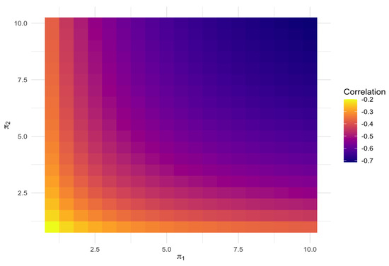
Figure 1.
Correlation plot for the Dirichlet distribution (5).
2.2.2. The Flexible Dirichlet Distribution
The following prior is represented by the flexible Dirichlet distribution as proposed by [8] and is expressed as a finite mixture of particular Dirichlet components. This distribution models multimodality and has shown to be capable of discriminating among many of the independence concepts relevant for compositional data.
Definition 2.
Suppose is distributed as flexible Dirichlet distribution. Then its pdf is given by
where is the vector with elements equal to zero except for the i-th that is equal to 1. The flexible Dirichlet also includes the Dirichlet as a special case if and , .
Figure 2 aims to show what role each of the parameters play in creating this flexible distribution. The first row of contours can be used as a base to compare the suggested changes against in order to illustrate the effects that each parameter has on the distribution form. The second row shows how increasing , from 3 to 7, splits the pdfs into different modes. The last row kept the larger but rearranged (by exchanging and ) and illustrates how this rearrangement flips the concentration of these modes. For this examples and was used for the first and second row with the third row represented by and . Figure 3 shows how the correlations changes as the values of and change. Specifically, no positive correlation is observed from this mixture structure of Dirichlet distributions.
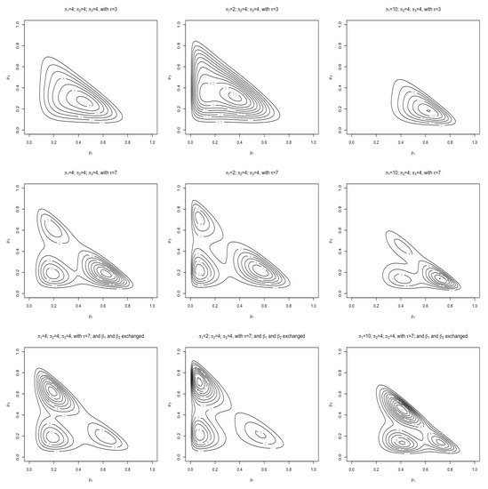
Figure 2.
Contour plots for the flexible Dirichlet distribution (6) with and for the first and second row and the third row represented by and .
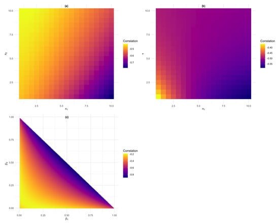
Figure 3.
Correlation plots for the flexible Dirichlet distribution (6). (a) Shows how the change in and affects the correlation, (b) how the change in affects the correlation and (c) shows how the change in and affects the correlation results.
2.2.3. The Double Flexible Dirichlet Distribution
The following prior is represented by the double flexible Dirichlet distribution as proposed by [9] and is a generalization of the Dirichlet structure which takes advantage of the finite mixture structure of the flexible Dirichlet distribution and also allows positive covariances. As such, potential positive correlation observed in a prior may be well modelled by this particular prior choice.
Definition 3.
Suppose is distributed as a double flexible Dirichlet distribution. Then its pdf is given by
where is the vector with elements equal to zero except for the i-th that is equal to 1.
Figure 4 shows the role that each of the parameters play in this flexible form while are similar. The first row of contours can be used as a reference to compare the changes against, while the second row shows how increasing from 3 to 7 splits the pdfs into multiple modes similar to what was seen in the flexible Dirichlet pdf (6). For this example . For Figure 5 were chosen to be less consistent () for the first row. For the second row the and the last being . By changing the values of we can see how the concentration of the modes changes.
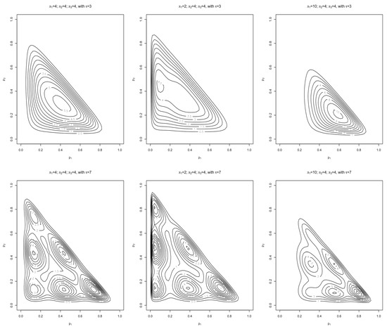
Figure 4.
Contour plots for the double flexible Dirichlet distribution (8). This figure shows the effect the value of (changing from 3 to 7) has on the distribution form.
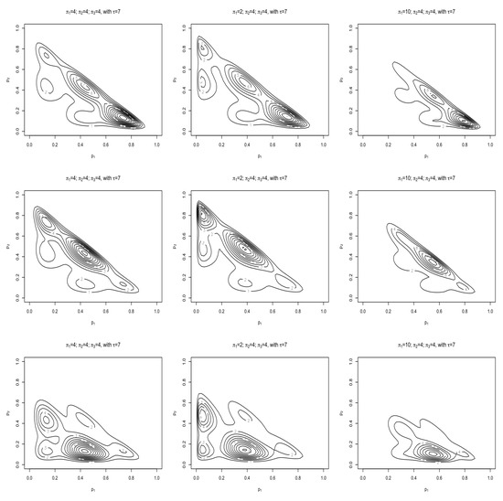
Figure 5.
Contour plots for the double flexible Dirichlet distribution (8). By changing the values of it can be seen how the concentrations of the different modes change.
Figure 6 shows how the correlations changes as the values of and change. The first correlation plot (a) speaks to the parameters in the first row of Figure 5 and investigate the effect that the change in has on the correlation. In (b) the parameters in the last row of Figure 5 were used and illustrates and it can be seen that the positive correlation is dependent on as also discussed in [9].
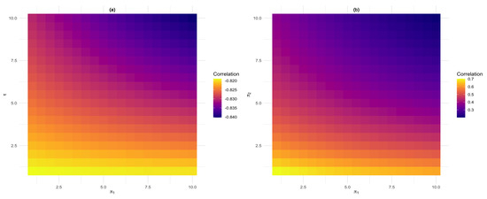
Figure 6.
Correlation plot for the double flexible Dirichlet distribution (8). (a) shows how the change in influences the correlation while we can see in (b) that the values of captures positive correlation.
3. Bayesian Estimation of Entropy
In this section the usual multinomial-Dirichlet setup is enriched with the additional consideration of the flexible Dirichlet- and double flexible Dirichlet mixtures ((6) and (8)) as priors for the multinomial likelihood. In this way, it allows the practitioner to obtain a posterior distribution from where closed form expressions for the entropies under consideration can be obtained, by particularly focussing on the product moment of the posterior model, in order to access the power sum functional under the assumption of squared error loss.
3.1. For the Dirichlet Prior
Theorem 1.
Since the complete product moments of the posterior distribution is of interest in order to determine the power sum (4) we are interested in .
Definition 4.
The definition of the complete product moment of a variable with pdf is given by [4]
Theorem 2.
Suppose that follows a Dirichlet posterior distribution with pdf given in (9). Then the complete product moment is given by
Proof.
Using the complete product moments derived in (11), the Bayesian estimator for the power sum (4) can be derived by setting with and .
Theorem 3.
The Bayesian estimator for the power sum functional under the Dirichlet posterior (9) is given by:
3.2. For the Flexible Dirichlet Prior
Theorem 4.
Proof.
By applying Bayes’s theorem (1) the numerator will have the following form:
The denominator of the posterior distribution will be given by
The second line of the above equation can be written as
Each integral is equal to 1, since it corresponds to the total probability of a Dirichlet distribution, hence the denominator will simplify to the following form:
In the case of the flexible Dirichlet (13) the following theorem derives the complete product moment as defined in (10).
Theorem 5.
Suppose that follows a flexible Dirichlet posterior distribution with pdf given in (13). Then the complete product moment is given by
Proof.
We identify that each integral in the above expression is of the form of the Dirichlet kernel. Using the definition of total probability, the result follows.
□
Using the complete product moments derived in (17), the Bayesian estimator for the power sum (4) can be derived by setting with and .
Theorem 6.
The Bayesian estimator for the power sum functional under the flexible Dirichlet posterior distribution (13) is given by:
3.3. For the Double Flexible Dirichlet Prior
Theorem 7.
Proof.
By applying Bayes’s theorem (1) the numerator will have the following form:
The denominator of the posterior will be given by
See that
Each integral is equal to 1, since it corresponds to the total probability of a Dirichlet distribution, hence the denominator will simplify to the following form:
□
Subsequently an expression for will be derived.
Theorem 8.
Suppose that follows a double flexible Dirichlet posterior distribution with pdf given in (20). Then the complete product moment is given by
where
and
Proof.
We identify that each integral in the above expression is of the form of the Dirichlet kernel. Using the definition of total probability, the result follows. □
Using the complete product moments derived in (24), the Bayesian estimator for the power sum (4) can be derived by setting with and .
Theorem 9.
The Bayesian estimator for the power sum functional under the double flexible Dirichlet posterior (20) is given by:
where
and
4. Evaluation and Discussion
The following is the exploratory approach to determining potential estimates from the posteriors (9), (13), and (20) by incorporating sample information via the correlation. The following steps [10] were used to determine the optimal values of the parameters of the various priors considered for the multinomial model, in conjunction with the data available and expert judgement. This exploratory approach serves to gain insight into parameter estimation in this Bayes context by utilising sample information via the correlation (which could be positive due to the inclusion of the double flexible Dirichlet distribution as prior).
- Create a grid by specifying all possible values for each parameter within the range specified in step 1. The grid will contain all possible combinations of these parameter options.
- For each step in the grid search, calculate the correlation for each parameter combination.
- When selecting the parameters of the prior distribution, choose them such that the parameters ensure a pre-determine range of entropy values. The entropy range can be selected when taking into consideration that lower entropy values are associated with less uncertainty and therefore higher concentrated distributions.
- Ensure that the resultant correlation for the range of possible estimates are in range of what is obtained from the data.
- Visually inspect the selected parameters to ensure a good fit.
The dataset that was considered, obtained from [15], was collected through household budget surveys aimed at studying consumer demand. This dataset was also used in studies such as [8] and reports the household expenditures (in Hong Kong Dollars) on two commodity groups of a sample of 40 individuals. The variables considered are the proportions spent on housing (including fuel and lights) (), consumables (including alcohol and tobacco) (), and the rest classified as services and other goods (including transport and vehicles, clothing, footwear, and durable goods). The results obtained are reported for for Tsallis, Generalized Mathai and Abe (see Table 1) and visually displayed to illustrate the fitted results.
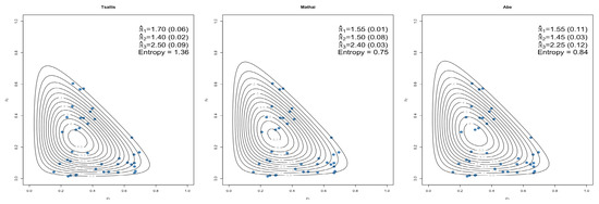
Figure 7.
Dirichlet Prior (5) estimated parameters and standard errors.
For equal weight was chosen as ( and ). Figure 8 shows how well the flexible Dirichlet prior (6) isolates the three modes visible within the data.
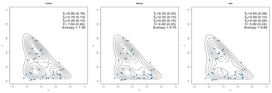
Figure 8.
Flexible Dirichlet Prior (6) estimated parameters and standard errors.
Figure 9 shows how the double flexible Dirichlet prior (8) fit the dataset with predetermined weight for the ().
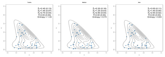
Figure 9.
Double flexible Dirichlet Prior (8) estimated parameters and standard errors.
The parameters of these different posterior distributions resulted in distributions which compared well to the observed data (some better than others) and also provided similar correlations than those found in the data. As it is known that the prior distribution plays a vital role in Bayesian analysis it is important to be able to quantify the impact of each prior in order to choose between one or more priors [7]. In order to measure the impact of the different priors, the WIM [7] was considered and reported in Table 2. These results were calculated by considering the estimated parameters as reported in Figure 7, Figure 8 and Figure 9 for each of the entropy measures investigated. The posterior distributions were then compared by calculating the WIM using the wasserstein1d function in R (statistical software).
Table 2.
Wasserstein Impact Measure results for each set of parameters estimated.
It can be seen that when comparing the WIM for each pair of posteriors considered, the measures resulting from the flexible and double flexible Dirichlet priors yielded large differences when compared to the Dirichlet distribution but almost no difference when comparing the two flexible distributions with each other. From the visual inspections and the WIM results is can be seen that there is value in considering generalizations of the Dirichlet distributions, in particular the considered mixtures of Dirichlet distributions. This may further benefit the practitioner in possible cases of clustering, then multimodal data may be present which the flexible Dirichlet- as well as the double flexible Dirichlet would be able to capture meaningfully.
5. Concluding Remarks
This paper considers key generalized entropy forms via the power sum functional of the posterior distribution, when subject to mixtures of Dirichlet distributions as a prior for the popular multinomial likelihood with K distinct classes. Here, the double flexible Dirichlet distribution offers the potential of positive prior correlation when this might be necessitated by prior information or expert opinion. Bayesian estimators were constructed for generalised entropy functions via this power sum functional, emanating from the product moment of each consider mixture of Dirichlet distribution’s prior, and implemented for parameter estimation when fitting posterior distributions to real economic data. Using the Bayesian estimates of these entropy measures proved to be a useful aid in selecting the prior distribution by consideration of the WIM, however, it is essential to evaluate each scenario separately. A possible further step of action may be to investigate possible other values of on the estimation. Further work include the potential probability representation of quantum states that can be characterised by the priors considered in this paper [16], as well as future interest in dimension-free estimation of entropy in relevant settings [17].
Author Contributions
Conceptualization, J.T.F.; methodology, J.T.F., T.B.; software, T.B.; validation, J.T.F., T.B., A.B.; formal analysis, J.T.F., T.B.; data curation, T.B.; writing—original draft preparation, T.B.; writing—review and editing, J.T.F., T.B., A.B.; supervision, J.T.F.; funding acquisition, J.T.F., T.B., A.B. The authors would like to thank three anonymous reviewers as well as the associate- and guest editors for their valuable feedback that led to an improved presentation of this paper. All authors have read and agreed to the published version of the manuscript.
Funding
The authors acknowledge the support of the Department of Statistics at the University of Pretoria, Pretoria, South Africa. This work enjoys support from the following grants: RDP296/2021 at the University of Pretoria; NRF ref. SRUG190308422768 nr. 120839; the DSTNRF South African Research Chair Initiative in Biostatistics UID: 114613; Statomet, University of Pretoria; as well as the Centre of Excellence in Mathematical and Statistical Sciences at the University of the Witwatersrand.
Institutional Review Board Statement
Not applicable.
Informed Consent Statement
Not applicable.
Data Availability Statement
The data under consideration in this study is in the public domain.
Conflicts of Interest
The funders had no role in the design of the study; in the collection, analyses, or interpretation of data; in the writing of the manuscript, or in the decision to publish the results.
References
- Lopes, A.M.; Machado, J.A.T. A review of fractional order entropies. Entropy 2020, 22, 1374. [Google Scholar] [CrossRef] [PubMed]
- Jiao, J.; Venkat, K.; Han, Y.; Weissman, T. Maximum likelihood estimation of functionals of discrete distributions. IEEE Trans. Inf. Theory 2017, 63, 6774–6798. [Google Scholar] [CrossRef]
- Butucea, C.; Issartel, Y. Locally differentially private estimation of functionals of discrete distributions. In Advances in Neural Information Processing Systems; Morgan Kaufmann Publishers: San Francisco, CA, USA, 2021; Volume 34. [Google Scholar]
- Botha, T.; Ferreira, J.T.; Bekker, A. Alternative Dirichlet Priors for Estimating Entropy via a Power Sum Functional. Mathematics 2021, 9, 1493. [Google Scholar] [CrossRef]
- Botha, T.; Ferreira, J.T.; Bekker, A. Some computational aspects of a noncentral Dirichlet family. In Innovations in Multivariate Statistical Modelling: Navigating Theoretical and Multidisciplinary Domains; Springer: New York, NY, USA, 2022. [Google Scholar]
- Arashi, M.; Bekker, A.; de Waal, D.; Makgai, S. Constructing Multivariate Distributions via the Dirichlet Generator. In Computational and Methodological Statistics and Biostatistics; Springer: New York, NY, USA, 2020; pp. 159–186. [Google Scholar]
- Ghaderinezhad, F.; Ley, C.; Serrien, B. The Wasserstein Impact Measure (WIM): A practical tool for quantifying prior impact in Bayesian statistics. Comput. Stat. Data Anal. 2021, 107352. [Google Scholar] [CrossRef]
- Ongaro, A.; Migliorati, S. A generalization of the Dirichlet distribution. J. Multivar. Anal. 2013, 114, 412–426. [Google Scholar] [CrossRef]
- Ascari, R.; Migliorati, S.; Ongaro, A. The Double Flexible Dirichlet: A Structured Mixture Model for Compositional Data. In Applied Modeling Techniques and Data Analysis 2: Financial, Demographic, Stochastic and Statistical Models and Methods; Wiley: New York, NY, USA, 2021; Volume 8, pp. 135–152. [Google Scholar]
- Bodvin, L.; Bekker, A.; Roux, J.J. Shannon entropy as a measure of certainty in a Bayesian calibration framework with bivariate beta priors: Theory and methods. S. Afr. Stat. J. 2011, 45, 171–204. [Google Scholar]
- Zamzami, N.; Bouguila, N. Hybrid generative discriminative approaches based on multinomial scaled dirichlet mixture models. Appl. Intell. 2019, 49, 3783–3800. [Google Scholar] [CrossRef]
- Manouchehri, N.; Rahmanpour, M.; Bouguila, N.; Fan, W. Learning of multivariate beta mixture models via entropy-based component splitting. In Proceeding of the 2019 IEEE Symposium Series on Computational Intelligence (SSCI), Xiamen, China, 6–9 December 2019; pp. 2825–2832. [Google Scholar]
- Contreras Rodríguez, L.; Madarro-Capó, E.J.; Legón-Pérez, C.M.; Rojas, O.; Sosa-Gómez, G. Selecting an Effective Entropy Estimator for Short Sequences of Bits and Bytes with Maximum Entropy. Entropy 2021, 23, 561. [Google Scholar] [CrossRef]
- Sánchez, L.E.; Nagar, D.; Gupta, A. Properties of noncentral Dirichlet distributions. Comput. Math. Appl. 2006, 52, 1671–1682. [Google Scholar] [CrossRef][Green Version]
- Cox, D.; Hinkley, D.; Rubin, D.; Silverman, B. Monographs on Statistics and Applied Probability; Springer: New York, NY, USA, 1984. [Google Scholar]
- Man’ko, O.V.; Man’ko, V.I. Probability representation of quantum states. Entropy 2021, 23, 549. [Google Scholar] [CrossRef] [PubMed]
- Cohen, D.; Kontorovich, A.; Koolyk, A.; Wolfer, G. Dimension-free empirical entropy estimation. In Advances in Neural Information Processing Systems; Morgan Kaufmann Publishers: San Francisco, CA, USA, 2021; Volume 34. [Google Scholar]
Publisher’s Note: MDPI stays neutral with regard to jurisdictional claims in published maps and institutional affiliations. |
© 2022 by the authors. Licensee MDPI, Basel, Switzerland. This article is an open access article distributed under the terms and conditions of the Creative Commons Attribution (CC BY) license (https://creativecommons.org/licenses/by/4.0/).