Small Area Estimation Using a Semiparametric Spatial Model with Application in Insurance

Abstract

Additional information and borrowing strength from the related sites and other sources will improve estimation in small areas. Generalized linear mixed-effects models (GLMMs) have been frequently used in small area estimation; however, the relationship between the response variable and some covariates may not be linear in many cases. In such cases, using semiparametric modeling, incorporating some nonlinear symmetric/asymmetric functions to the predictor seems more appropriate due to their flexibility. In addition, spatial dependence is observed between areas in many cases. Thus, using the semiparametric spatial models for small areas is of interest. This paper presents semiparametric spatial GLMMs and approximates the nonlinear component using splines to estimate the linear part. We apply our proposal for analyzing insurance data obtained from an Iranian insurance company. Our numerical illustrations will support the use of our proposal in situations where the spatial GLMMs may not be appropriate.

1. Introduction

Comprehensive information and appropriate statistical data are essential for planning, decision-making, and policymaking. Knowing the population requires having enough statistical information. Such information is generally obtained through surveys or censuses, typically designed for scientific purposes or population parameters (big areas). Nevertheless, for some reason, the available sample might not be enough to obtain a valid estimation in a small area or subdomain. These reasons include the lack of sufficient information in the target areas, the absence of pre-arranged planning while obtaining information, the lack of funding resources, statistical capacities, long periods between recording information, and some privacy laws. In such cases, the need for small area estimation is felt. The small area is a subdomain such as provinces, counties, and sub-populations such as specific age–sex race groups and health regions for which the sample size is not enough to obtain a valid estimation.

Statistically, the small amount of data in the small area (sometimes the sample size is zero) increases the prediction error. In such cases, the direct estimators are not accurate enough. To obtain a reliable estimation in the small area, the auxiliary information of the corresponding regions or the information of the same small area in previous study periods or extra information in the recorded statistics, administrative surveys, or a combination of these methods are used. The effect of areas on each other, which can be emerged by spatial correlation, can also be considered a valuable measure to increase estimation capabilities. In practice, the small area boundaries are contractual, and there is no reason why the effects in adjacent areas are not correlated. Therefore, it seems meaningful to test the assumption of spatial correlation of the closed regions.

In modeling the small area, valuable efforts have been made. Some of them are summarized as follows. Morales et al. [1] used the linear mixed model (LMM) to obtain the poverty ratio and the mean square prediction error (MSPE) of the small area estimator. Boubeta [2] used the Poisson regression model to estimate the small area parameter. Malee and Muller [3] present a semiparametric model to describe the geographic variability component. Chandra et al. [4] used a nonparametric generalized linear mixed model (GLMM) for non-Gaussian response variables when the data are spatially non-stationary in the small area and obtained MSE estimation for the nonlinear spline spatial model. Zhu et al. [5] considered the small area effect as an unknown function, estimated the small area using the semiparametric model, and represented the small area effect by the penalized spline. Torabi and Jiang [6] obtained an estimation of small area parameters using a spatial LMM. They used the conditional autoregressive (CAR) model to consider the spatial random effect. Torabi [7] studied the area-level spatial models in the small area. He used the proper CAR model to consider the spatial random effect of the areas and obtained the small area parameters using the spatial generalized linear model.

In this paper, our primary focus is on modeling insurance data. The insurance industry is one of the sectors for which the data analysis is placed in the category of the small area because data collecting is frequently encountered with many limitations. Life insurance has a special place among the various branches of the insurance industry due to its range of services. We intend to analyze life insurance data obtained from the database of Iran insurance companies in IRAN. These data were measured province-specifically from April to June 2018 for 32 provinces of Iran. The data include 466,759 observations. The response variable of interest for modeling is the provinces’ provincial per capita number of life insurance contracts. The explanatory variables in our analysis include the work experience of the insurance sales branch.

There are a few points to note in this data. (i) The small area estimation is generally divided into two categories: unit-level and area-level. For this data, the area level is considered due to the availability of the collected data. (ii) Due to the structure of the response variable in the study, which does not follow the normal distribution, using a kind of generalized linear models (GLMs) is unavoidable. (iii) Since the acceptance of life insurance in the basket of goods is related to income status and economic culture, and the borders between regions and provinces are contractual, there is no reason for the effects not to be interrelated in economic culture and income condition. Therefore, it seems logical to consider the correlation of regions in this study under the spatial dependence concept. (iv) As shown in Figure 1, the scatter plot of response versus explanatory variable depicts drastic fluctuations, which means that a linear trend cannot explain the relationship well. Moreover, since the relationship between response and covariate is unknown, it does not make sense to consider the parametric model. Thus, regression modeling must consider a nonlinear relationship between the response and the explanatory variable under the non-parametric component.

The points (i)–(iii) provide conditions to follow the work in [7]. However, the last point leads us to add a nonparametric part as a symmetric/asymmetric function to the model in [7]. Therefore, our main contribution is to propose a semiparametric spatial generalized linear mixed model in a small area, thereby increasing flexibility in the prediction. We derive the empirical best prediction (EBP) for the small area predictor and the mean squared prediction error (MSPE) for the EBP. We also consider the small area’s spatial random effects (SRE).

This paper is organized as follows: In Section 2, we present EBP to the small area predictor and obtain the MSPE of the EB estimator. In Section 3, the proposed methodology is applied to the real data on the provincial per capita number of life insurance contracts. After that, in Section 4, we present two simulation experiments and evaluate the performance of the proposed method. Section 5 offers some results and provides concluding remarks.

2. Semiparametric Mixed-Effects Model

Semiparametric mixed-effects modeling, combining a nonlinear function with the linear predictor, has a long history and dates back to Zeger and Diggle [8]. They used a semiparametric random intercept model to analyze the CD4 cell numbers in HIV seroconverts and estimated the nonparametric component by the backfitting method. Discussions about semiparametric models can be founded in Roozbeh [9,10], Akdeniz and Roozbeh [11], Taavoni and Arashi [12], and Taavoni et al. [13].

Suppose that the number of small areas and the number of explanatory variables are denoted by m and p, respectively. Under an area-level small area model, and in the framework of GLMs, it is assumed that the response variables are conditionally independent given the latent variable ${\mathit{\eta }}_i$, and follow the exponential families with the probability density:

$$f(y_i|{\mathit{\eta }}_i,\mathit{\varphi })=exp\{[y_i{\mathit{\eta }}_i-a({\mathit{\eta }}_i)]/\mathit{\varphi }+b(y_i,\mathit{\varphi })\},i=1,\cdots ,m,$$

(1)

where $y_i$ is the interested response variable in the ith small area, ${\mathit{\eta }}_i$ is the ith latent variable, and $\mathit{\varphi }$ is the scale parameter. Furthermore, $a(·)$ and $b(·)$ are known functions. Implementing statistical inferences on the latent variable ${\mathit{\eta }}_i$ is the objective of the small-area estimation. The model of the latent variable is defined as follows:

$${\mathit{\eta }}_i={\mathbf{x}}_i^{\top }\mathit{\beta }+{\mathbf{z}}_i^{\top }\mathbf{u}+f({\mathbf{t}}_i),$$

(2)

where ${\mathit{\eta }}_i$ is a function of $\mathrm{E}(y_i|\mathbf{u})$, ${\mathbf{x}}_i^{\top }$ is the ith row of the design matrix ${\mathbf{X}}_{m\times p}$, ${\mathit{\alpha }}_1={\mathit{\beta }}_{p\times 1}$ is the vector of unknown regression coefficients, and ${\mathbf{z}}_i^{\top }$ is the ith row of the identity matrix ${\mathbf{Z}}_{m\times m}$. The $\mathbf{u}=(u_1,\dots ,u_m)|{\mathit{\alpha }}_2$ is the vector of spatial random effect accompanied by distribution $\mathrm{MVN}(\mathbf{0},{\mathsf{\Sigma }}_{\mathbf{u}}({\mathit{\alpha }}_2))$ and $\mathit{\alpha }=({\mathit{\alpha }}_1^T,{\mathit{\alpha }}_2^T)$. In this model, we assume that the relation of the $f(\mathbf{t})$ with the response variable is nonlinear. Thus, it is considered a nonparametric component. The function $f(·)$ is generally unknown, but it is assumed that it is a smooth nonlinear function and has the second derivative. The estimation of nonparametric function f is presented as below:

$$f(\mathbf{t})=B_0+B_{1}t+B_2{t}^2+\cdots +B_d{t}^d+B_{d+1}{(t-t_1)}_{+}^d+\cdots +B_{d+k}{(t-t_k)}_{+}^d,$$

(3)

which is called a d-order spline estimator function with knots $t_1,\dots ,t_k$. In this function, $B_0,\dots ,B_{d+k}$ are spline regression coefficients (refer to [14] for more details). Further, ${(.)}_{+}^d$ denotes the truncated polynomial basis function of order d defined as:

$${(t-t_i)}_{+}^d=\left\{\begin{array}{cc}{(t-t_i)}^d,\hfill & t>t_i,\hfill \\ 0,\hfill & O.W.\hfill \end{array}\right.$$

The approximation function in (3) can be summarized by $f(\mathbf{t})={\mathbf{w}}^{\top }\mathbf{B}$, which ${\mathbf{B}}^{\top }=(B_0,B_1,\dots ,B_h)$; $h=d+k+1$ is a vector of spline regression coefficients and $\mathbf{W}={(1,t,\dots ,t^d,{(t-t_1)}_{+}^d,\dots ,{(t-t_k)}_{+}^d)}^{\top }$. Thus, Equation (2) can be rewritten as:

$${\mathit{\eta }}_i={\mathbf{x}}_i^{\top }\mathit{\beta }+{\mathbf{z}}_i^{\top }\mathbf{u}+{\mathbf{w}}_i^{\top }\mathbf{B}.$$

(4)

By combining the fixed and spline effects in (4), the following equation is resulted:

$${\mathit{\eta }}_i={\tilde{\mathbf{x}}}_i^{\top }\mathit{\theta }+{\mathbf{z}}_i^{\top }\mathbf{u},$$

(5)

wherein ${\tilde{\mathbf{x}}}_i=({\mathbf{x}}_i,{\mathbf{W}}_i)$ is the mixed design $(p+h)\times m$ matrix of the fixed effects and spline effects, and $\mathit{\theta }={(\mathit{\beta },\mathbf{B})}^{\top }$ is the $(p+h)\times 1$ vector of the regression coefficients corresponding to fixed and spline effects.

In order to predict the latent variable ${\mathit{\eta }}_i$, the conditional density is calculated using the equation below:

$$g({\mathit{\eta }}_i|y_i,\mathit{\alpha })\propto exp\{\frac{-{\mathit{\eta }}_i^2}{2{\sigma }_{{\mathit{\eta }}_i}^2}+\frac{{\mathit{\eta }}_i({\tilde{\mathbf{x}}}_i\mathit{\theta })}{{\sigma }_{{\mathit{\eta }}_i}^2}+\frac{[y_i{\mathit{\eta }}_i-a({\mathit{\eta }}_i)]}{{\mathit{\eta }}_i\mathit{\varphi }}\},$$

(6)

where ${\sigma }_{{\mathit{\eta }}_i}^2={\mathbf{z}}_i^{\top }\mathsf{\Sigma }{\mathbf{z}}_i$ and $\mathit{\alpha }$ is the vector of parameter of random effects. The Laplace approximation centered around the point ${\mathit{\eta }}_i^0=\arg {max}_{{\mathit{\eta }}_i}g({\mathit{\eta }}_i|y,\mathit{\alpha })$ is used to approximate the conditional density of ${\mathit{\eta }}_i$ [15]:

$$[y_i{\mathit{\eta }}_i-a({\mathit{\eta }}_i)]\approx [y_i{\mathit{\eta }}_i^0-a({\mathit{\eta }}_i^0)]+\left({\mathit{\eta }}_i-{\mathit{\eta }}_i^0\right)\left[y_i-a{}^{\prime }\left({\mathit{\eta }}_i^0\right)\right]-\frac{1}{2}\left({\mathit{\eta }}_i-{\mathit{\eta }}_i^0\right)2a^{″}\left({\mathit{\eta }}_i^0\right),$$

(7)

Proposition 1.

Under the conditions that the first and second derivatives of $\mathit{\alpha }({\mathit{\eta }}_i)$ in Equation (7) are available in the closed-form, the conditional density of ${\mathit{\eta }}_i$ becomes a normal approximation with conditional mean $\mathrm{E}({\mathit{\eta }}_i|y_i,\mathit{\alpha })$ and conditional variance $\mathrm{var}({\mathit{\eta }}_i|y_i,\mathit{\alpha })$, given by:

$$\begin{array}{cc}\hfill \mathrm{E}({\mathit{\eta }}_i|y_i,\mathit{\alpha })& ={\tilde{\mathbf{x}}}_i^{\top }\mathit{\theta }+{\mathbf{z}}_i^{\top }{\mathsf{\Sigma }}_{\mathbf{u}}{\mathbf{R}}^{-1}\left[l(\mathbf{y},{\mathit{\eta }}^0)-\widetilde{\mathbf{X}\mathit{\theta }}\right],\hfill \end{array}$$

(8a)

$$\begin{array}{cc}\hfill \mathrm{var}({\mathit{\eta }}_i|y_i,\mathit{\alpha })& ={\mathbf{z}}_i^{\top }\left[{\mathsf{\Sigma }}_{\mathbf{u}}-{\mathsf{\Sigma }}_{\mathbf{u}}{\mathbf{R}}^{-1}\mathbf{Z}{\mathsf{\Sigma }}_{\mathbf{u}}\right]{\mathbf{z}}_i,\hfill \end{array}$$

(8b)

where $\mathbf{R}=\mathbf{Z}{\mathsf{\Sigma }}_{\mathbf{u}}{\mathbf{Z}}^{\top }+\mathbf{P}$, $\mathbf{P}$ is a diagonal matrix with entries ${\mathbf{P}}_{i,i}=\frac{\mathit{\varphi }}{a^{″}({\mathit{\eta }}_i^0)}$, ${\mathit{\eta }}^0={({\mathit{\eta }}_1^0,\dots ,{\mathit{\eta }}_m^0)}^{\top }$, and $l(y_i,{\mathit{\eta }}_i^0)=\left[y_i-a{}^{\prime }({\mathit{\eta }}_i^0){\mathit{\eta }}_i^0{a}^{″}({\mathit{\eta }}_i^0)\right]/a^{″}({\mathit{\eta }}_i^0)$ for $i=1,\dots ,m$ and ${\mathit{\eta }}^0=argma{x}_{{\mathit{\eta }}_i}f(y_i|{\mathit{\eta }}_i,\mathit{\varphi })$. For the proof, refer to Appendix A.

If $\mathit{\alpha }$ is known, the best predictor of the ${\mathit{\eta }}_i$ is the conditional expectation ($\mathrm{E}({\mathit{\eta }}_i|y_i,\mathit{\alpha })={\tilde{\mathit{\eta }}}_i^B={\tilde{\mathit{\eta }}}_i^B(\mathit{\alpha },y_i)$) and the second-order unbiased mean squared prediction errors is $\mathrm{var}({\mathit{\eta }}_i|y_i,\mathit{\alpha })$, which was defined in Equation (8a,b). However, when $\mathit{\alpha }$ is the vector of unknown parameters, we obtained the best empirical prediction of ${\mathit{\eta }}_i$ by replacing $\mathit{\alpha }$ by $\widehat{\mathit{\alpha }}$. Frequentist and Bayesian methods are generally used to process spatial generalized linear mixed models (SGLMMs). Due to the computational complexity in calculating maximum likelihood estimation (MLE), frequency methods require numerical solutions of high-dimensional and intractable integrals. In this paper, the MLE method is impossible due to the need to solve high-dimensional integrals. In addition, using Bayesian methods always faces the problem of selecting the appropriate prior. According to the problems mentioned in the two Frequency and Bayesian methods, the data cloning (DC) approach (see [16]) has been used to estimate the unknown parameters. DC is a computational method for calculating MLE, using MCMC (Markov chain Monte Carlo) algorithm and Bayesian methods. This method does not require numerical maximization and derivation of a complex function, which is robust to the prior choice. To see more Bayesian studies, refer to [17,18,19].

To understand the logic of the DC method, consider that the observations of $\mathbf{y}=(y_1,\dots ,y_m)$ and the explanatory variables are independently repeated exactly k times. The vector of random effects, by using their probabilistic explanations, generated k times, so that ${\mathbf{y}}^k=({\mathbf{y}}^T,{\mathbf{y}}^T,\dots ,{\mathbf{y}}^T)$ represents the data at k times of repetition. The maximum likelihood function ${\mathbf{y}}^k$ is ${L(\mathit{\alpha };\mathbf{y})}^k=L^k(\mathit{\alpha };\mathbf{y})$ where the likelihood function $L(\mathit{\alpha };\mathbf{y})$ is the likelihood of original data. Since the DC method is based on the asymptotic behavior of posterior density, the theoretical conditions of asymptotic posterior density can be established by increasing the sample size. In this approach, the posterior distribution of the clone answer is shown as:

$${\mathsf{\Pi }}_k(\mathit{\alpha }|{\mathbf{y}}^k)=\frac{L^k(\mathit{\alpha };\mathbf{y})\mathsf{\Pi }(\mathit{\alpha })}{c({\mathbf{y}}^k)},$$

(9)

where $c({\mathbf{y}}^k)=\int L^k(\mathit{\alpha },\mathbf{y})\mathsf{\Pi }(\mathit{\alpha })\mathrm{d}\mathit{\alpha }$ and $\mathsf{\Pi }(\mathit{\alpha })$ are the normalized constant and prior distribution, respectively. Lele et al. [16] show that under some regular conditions, the posterior distribution of $\sqrt{k}{\mathsf{\Sigma }}^{-1/2}(\mathit{\alpha }-\widehat{\mathit{\alpha }})|{\mathbf{y}}^k$ converges to a multivariate normal distribution with mean $\mathbf{0}$ and identity covariance matrix $\mathbf{I}$. Thus, the estimation of $\mathit{\alpha }$ is the mean of posterior density under the squared error loss function. The mean squared empirical prediction error is approximately calculated as below:

$$\begin{array}{ccc}\hfill \mathrm{MSPE}({\widehat{\mathit{\eta }}}_i^{EB})& =& \mathrm{E}\left\{{\left({\widehat{\mathit{\eta }}}_i^{EB}-{\mathit{\eta }}_i\right)}^2\right\}=\mathrm{E}\left\{{\left({\tilde{\mathit{\eta }}}_i^B-{\tilde{\mathit{\eta }}}_i^B+{\widehat{\mathit{\eta }}}_i^{EB}-{\mathit{\eta }}_i\right)}^2\right\}\hfill \\ & =& \mathrm{E}\left\{{\left({\tilde{\mathit{\eta }}}_i^B-{\mathit{\eta }}_i\right)}^2\right\}+\mathrm{E}\left\{{\left({\tilde{\mathit{\eta }}}_i^{EB}-{\tilde{\mathit{\eta }}}_i\right)}^2\right\}\hfill \\ & =& g_{1i}(\mathit{\alpha })+tr\left\{\mathrm{E}\left[\left(\frac{\partial {\tilde{\mathit{\eta }}}_i^B(\mathit{\alpha },y_i)}{\partial \mathit{\alpha }}\right){\left(\frac{\partial {\tilde{\mathit{\eta }}}_i^B(\mathit{\alpha },y_i)}{\partial \mathit{\alpha }}\right)}^{\top }\right]\mathrm{E}(\widehat{\mathit{\alpha }}-\mathit{\alpha }){(\widehat{\mathit{\alpha }}-\mathit{\alpha })}^{\top }\right\}+o\left(m^{-1}\right).\hfill \end{array}$$

In the above relation, $o\left(m^{-1}\right)$ is the “little-o” notation for the asymptotic behaviour so that $a(n)=o(n)$ means ${lim}_{n\to \infty }\frac{a(n)}{n}=0$. Further, $\mathrm{E}\{·\}$ denotes the mathematical expectation with respect to ${\mathit{\eta }}_i$. Then,

$$\mathrm{MSPE}\left({\widehat{\mathit{\eta }}}_i^{EB}\right)=g_{1i}(\mathit{\alpha })+g_{2i}(\mathit{\alpha })+o\left(m^{-1}\right),$$

(10)

where,

$$\begin{array}{ccc}\hfill g_{1i}(\mathit{\alpha })& =& \mathrm{E}\left\{{\left({\tilde{\mathit{\eta }}}_i^B-{\mathit{\eta }}_i\right)}^2\right\},\hfill \\ \hfill g_{2i}(\mathit{\alpha })& =& tr\left\{\mathrm{E}\left[\left(\frac{\partial {\tilde{\mathit{\eta }}}_i^B(\mathit{\alpha },y_i)}{\partial \mathit{\alpha }}\right){\left(\frac{\partial {\tilde{\mathit{\eta }}}_i^B(\mathit{\alpha },y_i)}{\partial \mathit{\alpha }}\right)}^{\top }\right]\mathrm{E}(\widehat{\mathit{\alpha }}-\mathit{\alpha }){(\widehat{\mathit{\alpha }}-\mathit{\alpha })}^{\top }\right\},\hfill \end{array}$$

(11)

where $tr\left\{A\right\}$ denotes the trace of matrix A. It can be seen that $\mathrm{MSPE}$ of ${\widehat{\mathit{\eta }}}_i^{EB}$ is a function of unknown parameters $\mathit{\alpha }$. By replacing $\mathit{\alpha }$ by $\widehat{\mathit{\alpha }}$, Torabi [7] noticed that in this estimation, the rough value for $\mathrm{MSPE}\left({\widehat{\mathit{\eta }}}_i^{EB}\right)$ is approximately equal to $\mathrm{E}\left(\widehat{\mathrm{MSPE}}\left({\widehat{\mathit{\eta }}}_i^{EB}\right)\right)$, where

$$\begin{array}{ccc}\hfill \widehat{\mathrm{MSPE}}\left({\widehat{\mathit{\eta }}}_i^{EB}\right)& =& g_{1i}(\widehat{\mathit{\alpha }})-{\left[\frac{\partial g_{1i}(\mathit{\alpha })}{\partial \mathit{\alpha }}\right]}^{\top }\mathrm{E}(\widehat{\mathit{\alpha }}-\mathit{\alpha })-\frac{1}{2}\mathrm{tr}\left\{\left[\frac{{\partial }^2{g}_{1i}(\mathit{\alpha })}{\partial \mathit{\alpha }\partial {\mathit{\alpha }}^{\top }}\right]\mathrm{E}(\widehat{\mathit{\alpha }}-\mathit{\alpha }){(\widehat{\mathit{\alpha }}-\mathit{\alpha })}^{\top }\right\}\hfill \\ & & +\mathrm{tr}\left\{\mathrm{E}\left[\left(\frac{\partial {\tilde{\mathit{\eta }}}_i^B(\mathit{\alpha },y)}{\partial \mathit{\alpha }}\right){\left(\frac{\partial {\tilde{\mathit{\eta }}}_i^B(\mathit{\alpha },y)}{\partial \mathit{\alpha }}\right)}^{\top }\right]\mathrm{E}(\widehat{\mathit{\alpha }}-\mathit{\alpha }){(\widehat{\mathit{\alpha }}-\mathit{\alpha })}^{\top }\right\}.\hfill \end{array}$$

(12)

It is noticeable that sometimes the calculated value of $\mathrm{E}\left(\widehat{\mathrm{MSPE}}\left({\widehat{\mathit{\eta }}}_i^{EB}\right)\right)$ can be negative. In this case, Prasad and Rao [20] replaced negative values with positive values.

3. Life Insurance Data Analysis

Here, we model the above-mentioned number of life insurance contract data using the proposed semiparametric spatial generalized linear mixed-effects model. We consider the following spatial Poisson regression model:

$$\begin{array}{ccc}\hfill y_i& \sim & \mathrm{Poisson}({\lambda }_i),\hfill \\ \hfill log({\lambda }_i)& =& \mathit{\beta }+{\mathbf{z}}_i^{\top }\mathbf{u}+f(E_i),\hfill \end{array}$$

where $y_i$ is the reported mean number of life insurance contracts of the ith province in Iran, $\mathit{\beta }$ is defined as an intercept, ${\mathbf{z}}_i^{\top }$ is the ith row of the identity matrix, and $\mathbf{u}$ is taken from an ICAR(intrinsic conditional autoregressive) model [21]. Further, $E_i$ is the mean of work experience of the insurance sales branch of the ith province. It seems that the $E_i$ and the response variable have a nonlinear relationship, and it is not meaningful to insert it as a parametric component. Therefore, we consider it as a nonparametric function $f(E_i)$ into the model where f is a smooth and unknown function of duration. We use the spline approximation method to approximate the nonparametric component.

Here, the function $f(\mathbf{E})$ is a cubic spline with evenly spaced knots in the range of $\mathbf{E}$, at the points of $22.53918$, $23.43646$, and $24.35712$. This can be summarized by $f(\mathbf{E})={\mathbf{B}}^{\top }\mathbf{W}$, in which ${\mathbf{B}}^{\top }=(B_0,B_1,\dots ,B_h)$; $h=d+k+1=3+3+1=7$ are spline regression coefficients and

$$\mathbf{W}=(1,t,t^2,t^3,{(t-22.53918)}_{+}^3,{(t-23.43646)}_{+}^3,{(t-24.35712)}_{+}^3).$$

Hence, the semiparametric spatial mixed model is derived as:

$$log({\lambda }_i)={\mathbf{x}}_i^{\top }\mathit{\beta }+{\mathbf{z}}_i^{\top }\mathbf{u}+{\mathbf{B}}_i^{\top }\mathbf{W}.$$

By combining the fixed and spline effects, the above model can be rewritten as:

$$log({\lambda }_i)={\tilde{\mathbf{x}}}_i^{\top }\mathit{\theta }+{\mathbf{z}}_i^{\top }\mathbf{u},$$

where the $8\times 32$ design matrix ${\tilde{\mathbf{x}}}_i=({\mathbf{x}}_i,{\mathbf{w}}_i)$ is the mixed of the fixed effect and Spline effects matrices, and $\mathit{\theta }={(\mathit{\beta },\mathbf{B})}^{\top }$ is an eight-dimensional vector of parameters of the regression coefficients and spline coefficients.

The estimation of the model parameters, which were found by data cloning, are presented in

Table 1. Model parameter estimates for the semiparametric spatial GLMM.

Parameter	Estimate	Standard Error
$\mathit{\beta }$	−0.1498	0.02699
$B_0$	−0.1915	0.06451
$B_1$	0.06252	0.01494
$B_2$	−0.01838	0.06013
$B_3$	−0.0603	0.0588
$B_4$	−0.01853	0.07475
$B_5$	0.02873	0.04812
${\lambda }_u$	0.2397	0.01419

. Here, the estimate of regression coefficient, spline coefficients $(B_0,\dots ,B_5)$, and spatial parameter ${\lambda }_u$ along with the respective standard errors are given.

To evaluate the flexibility and the effect of the duration contract in a nonlinear manner, which leads to an increase in the flexibility of the model, we compare the above-suggested model with the following alternative model:

$$log({\lambda }_i)=E_i+\mathit{\beta }+{\mathbf{z}}_i^{\top }\mathbf{u}.$$

Figure 2 depicts the boxplot of $\mathrm{MSPE}$ of the ${\mathit{\eta }}_i^{EB}$ for the number of life insurance contracts in IRAN. As can be seen, the MSPE of EBP in the proposed model is smaller than the spatial generalized linear mixed model, thus, the suggested model transparently provides a smoother prediction attaining better results.

4. Simulation Study

This section uses the semiparametric mixed-effect model to evaluate the proposed method. Since this article expands Torabi’s proposed model [7], we have utilized the same Minnesota country map to compare our proposed model accuracy with the parametric model. The simulated data are obtained from the following model:

$$\begin{array}{ccc}\hfill y_i& \sim & \mathrm{Poisson}({\lambda }_i),\hfill \\ \hfill log({\lambda }_i)& =& log{n}_i+\mathit{\beta }+{\mathbf{z}}_i^{\top }\mathbf{u}+f(x_i),\hfill \end{array}$$

where $\mathbf{u}$ is generated from the ICAR model. The other components of this pattern have the following specifications: $n_i=30$ is the offset and $\mathit{\beta }=0.001$ is the intercept. $f(x)=1+2x-3sin(x)$ is the nonlinear function and $x_i$ is the fixed duration of the study generated from the uniform distribution on $(-3,3)$. First, we generate $\mathbf{u}$ from the ICAR distribution with parameters ${\lambda }_u=0.5$ for $i=1,\dots ,87$. We do this job independently for $R=1000$ steps and denote ${\mathbf{u}}^{(r)}$, $r=1,\dots ,R$ as the rth spatial random variable generated by $\mathbf{u}$. Inserting ${\mathbf{u}}^{(r)}$ in the formula $log\left({\lambda }_i^{(r)}\right)=log{n}_i+\mathit{\beta }+{\mathbf{z}}_i^{\top }{\mathbf{u}}^{(r)}+f(x)$ and getting ${\lambda }_i^{(r)}$ for each step, $y_i^{(r)}$ is generated from the Poisson distribution with mean ${\lambda }_i^{(r)}$ for $i=1,\dots ,87$ and $r=1,\dots ,R$.

For each simulation run, based on (2), we find:

$${\widehat{\mathit{\eta }}}_i^r=log{n}_i+\mathit{\beta }+{\mathbf{z}}_i^{\top }{\mathbf{u}}^{(r)}+f(x_i).$$

By using the data cloning approach, ${\widehat{\mathit{\eta }}}_i^{EB}$ is given by:

$${\widehat{\mathit{\eta }}}_i^{EB}=\mathrm{E}({\mathit{\eta }}_i|y_i,\mathit{\alpha })={\mathbf{x}}_i^{\top }\mathit{\theta }+{\mathbf{z}}_i^{\top }{\mathsf{\Sigma }}_u{\mathbf{Z}}^{\top }{\mathbf{R}}^{-1}\left[l(\mathbf{y},{\mathit{\eta }}^0)-\tilde{\mathbf{X}}\mathit{\theta }\right],i=1,\dots ,87,$$

where $\mathit{\theta }$ is a vector of regression and spline coefficients, ${\mathbf{z}}_i$ is the ith row of the identity matrix, ${\mathsf{\Sigma }}_u$ is the ICAR covariance matrix and ${\tilde{\mathbf{x}}}_i$ is the ith row of the $87\times 8$ matrix $\tilde{\mathbf{X}}$. The ${\widehat{\mathit{\eta }}}_i^{EB}$ is obtained for each of the 1000 steps. $\mathbf{R}$ and $l(.)$ are calculated as follows:

$$\begin{array}{ccc}\hfill f(y_i|{\mathit{\eta }}_i,\mathit{\varphi })& =& \left[{\mathrm{e}}^{-\lambda }{\lambda }^{y_i}\right]/y_i!\hfill \\ & =& exp\{y_i\ln \lambda -\lambda -\ln y_i!\},\hfill \\ \hfill a{}^{\prime }({\mathit{\eta }}_i^0)& =& \frac{\partial a{}^{\prime }({\mathit{\eta }}_i)}{\partial {\mathit{\eta }}_i}{|}_{{\mathit{\eta }}_i={\mathit{\eta }}_i^0}=\frac{\partial {\mathrm{e}}^{{\mathit{\eta }}_i}}{\partial {\mathit{\eta }}_i}{|}_{{\mathit{\eta }}_i={\mathit{\eta }}_i^0}={\mathrm{e}}^{{\mathit{\eta }}_i^0},\hfill \\ \hfill {\mathbf{P}}_{ii}& =& \frac{\mathit{\varphi }}{a^{″}({\mathit{\eta }}_i^0)}=\frac{1}{{\mathrm{e}}^{{\mathit{\eta }}_i^0}},\hfill \\ \hfill \mathbf{R}& =& \mathbf{Z}{\mathsf{\Sigma }}_u{\mathbf{Z}}^{\top }+\mathbf{P},\hfill \\ \hfill l(y_i,{\mathit{\eta }}_i^0)& =& [y_i-a{}^{\prime }({\mathit{\eta }}_i^0)+{\mathit{\eta }}_i^0{a}^{″}({\mathit{\eta }}_i^0)]/a^{″}({\mathit{\eta }}_i^0)=\frac{y_i-{\mathit{\eta }}_i^0+{\mathit{\eta }}_i^0{\mathrm{e}}^{{\mathit{\eta }}_i^0}}{{\mathrm{e}}^{{\mathit{\eta }}_i^0}},\hfill \end{array}$$

also the empirical MSPE (EMSPE) of ${\widehat{\mathit{\eta }}}_i^{EB}$ is calculated by using the following formula:

$$\mathrm{EMSPE}\left({\widehat{\mathit{\eta }}}_i^{EB}\right)=\frac{1}{R}\sum _{r=1}^R{\left[{\widehat{\mathit{\eta }}}_i^{EB(r)}-{\mathit{\eta }}_i^{(r)}\right]}^2,$$

To evaluate the performance of the proposed model, we compare it with the model $log({\lambda }_i)={\mathit{\beta }}_0+{\mathbf{x}}_i^{\top }\mathit{\beta }+{\mathbf{z}}_i^{\top }\mathbf{U}$. The estimation of model parameters by the DC method is reported in

Table 2. Model parameter estimates and corresponding standard errors using the MLE approach for the semiparametric spatial Poisson model.

Parameter	Estimate	Standard Error
$\mathit{\beta }$	−76.0308	22.10532
$B_0$	69.5480	22.31195
$B_1$	75.4873	22.03408
$B_2$	73.3040	22.15233
$B_3$	72.5719	22.08202
$B_4$	77.8309	22.12026
$B_5$	78.4698	22.10168
${\lambda }_u$	1.2003	0.17648

and

Table 3. Model parameter estimates and corresponding standard errors using the MLE approach for the parametric spatial Poisson model.

Parameter	Estimate	Standard Error
${\mathit{\beta }}_0$	−2.4955	0.05152
${\mathit{\beta }}_1$	0.8918	0.03687
${\lambda }_u$	0.1378	0.01313

for the proposed and parametric models.

Table 2 contain the estimates of regression coefficients, spline regression coefficients, and spatial parameter ${\lambda }_u$ for the semiparametric spatial Poisson model. Moreover, the results of the parametric model are shown in Table 3.

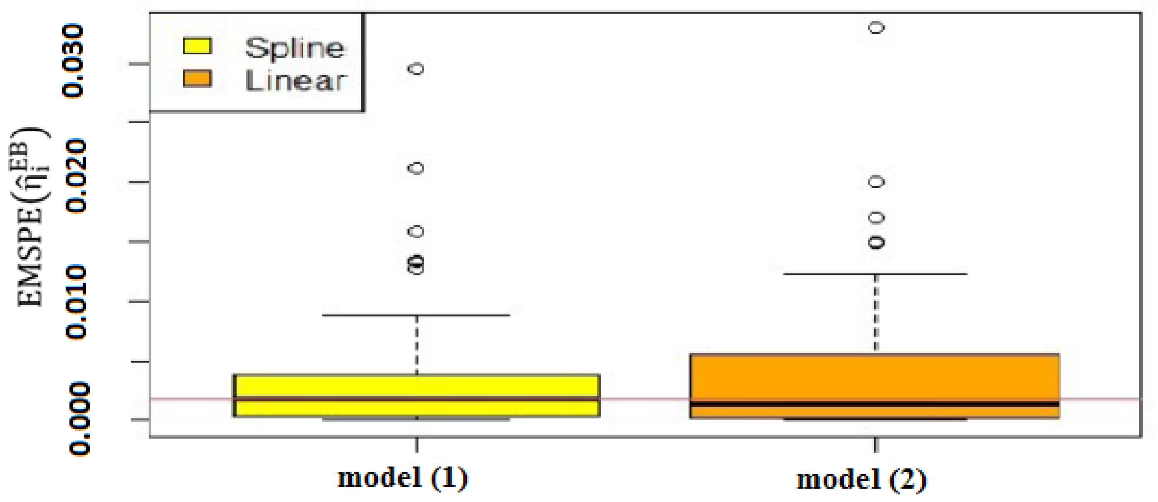
To evaluate the performance of the semiparametric spatial Poisson model, the box plots of EMSPE of ${\widehat{\mathit{\eta }}}_i^{EB}$ values are depicted in Figure 3, which shows the distribution of the mean square prediction error. As can be seen, the EMSPE of ${\widehat{\mathit{\eta }}}_i^{EB}$ in the proposed model is smaller than the parametric counterpart. The third quantile and maximum point of EMSPE of ${\widehat{\mathit{\eta }}}_i^{EB}$ in the proposed model are less than the parametric model. The maximum outlier points of EMSPE of ${\widehat{\mathit{\eta }}}_i^{EB}$ in the proposed model is less than the parametric model, which shows that the proposed model has better performance even in the outlier. Furthermore, the MSPE and ISQR values for these two models are listed in

Table 4. Value of the EMSPE of ${\widehat{\mathit{\eta }}}_i^{EB}$ and ISQR for the semiparametric and parametric spatial Poisson models.

	Semiparametric	Parametric
$\mathrm{MSPE}$	$0.009085778$	$0.02691221$
$\mathrm{ISQR}$	$0.009277414$	$0.02369608$

. This table shows the superiority of our proposed model. As a result, the semiparametric model improves the model in terms of prediction.

In Figure 3, the box plot of MSPE of ${\widehat{\mathit{\eta }}}_i^{EB}$ is shown in total areas. In a small area, MSPE of ${\widehat{\mathit{\eta }}}_i^{EB}$ is important not only in all areas but also in each area. In some cases, in the small area approach, some regions are more important, and those regions should be investigated more carefully. Hence, in order to compare the performance of the proposed model against the parametric model, the heat map of EMSPE of ${\widehat{\mathit{\eta }}}_i^{EB}$ is drawn separately by the province in Minnesota in Figure 4.

As shown in Figure 4, in some provinces, the MSPE of ${\widehat{\mathit{\eta }}}_i^{EB}$ in the proposed model are less than the MSPE of ${\widehat{\mathit{\eta }}}_i^{EB}$ in the parametric model and they are equal in some provinces. There is no area in which the MSPE of ${\widehat{\mathit{\eta }}}_i^{EB}$ in the proposed model is more than the parametric model.

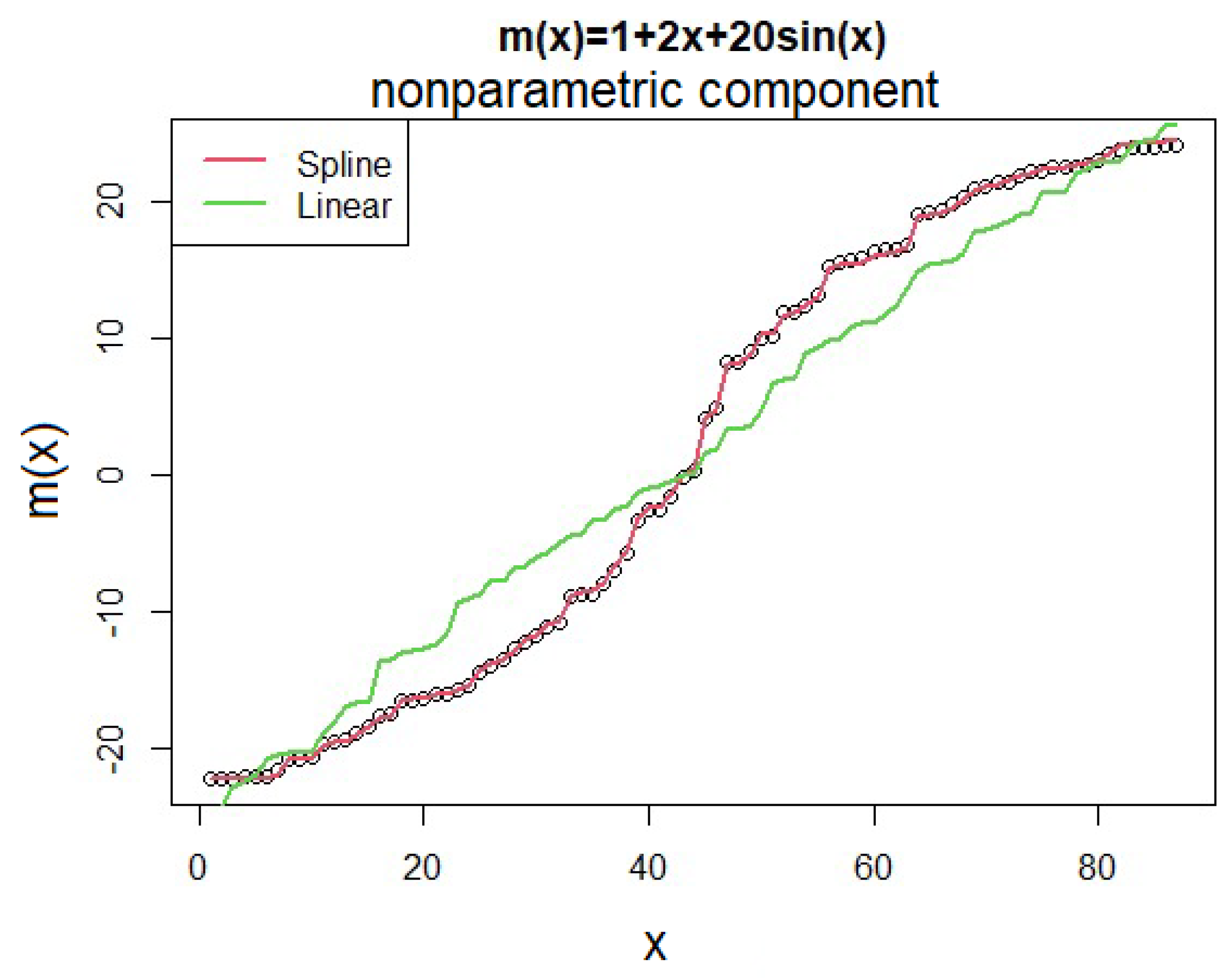
In addition to comparing the MSPE of ${\widehat{\mathit{\eta }}}_i^{EB}$, plotting the predicted values of two models versus simulated data can provide a better understanding of the performance of two models. As shown in Figure 5, the semiparametric model is more efficient than the parametric model in estimating the nonparametric component.

5. Conclusions

The GLMMs and linear mixed-effects models are the models that are frequently used in small areas. As we demonstrated in the analysis of life insurance data obtained from an Iran Insurance Company in IRAN, a nonlinear relation may exist between the response variable and some of the covariates. In such cases, the GLM models do not have the necessary capability, and new models are needed to analyze such a data set in a small area. A semiparametric spatial generalized linear mixed-effects model (GLMM) is proposed in the small area for normal and non-normal responses. The empirical best predictor for the small area parameters and the MSPE of the EBP of small area predictors were obtained. Life insurance data analysis demonstrated the superiority of the proposed model compared to the parametric spatial Poisson model. There is still room to explore more for the future. Other estimation methods, such as backfitting and kernel approaches, can be considered for future directions. In this paper, only one nonlinear element was added to the linear predictor of the spatial model. It is worth considering an additive structure for the nonlinear component and developing an additive semiparametric spatial GLMM.

References

1. Morales, D.; Pagliarella, M.C.; Salvatore, R. Small area estimation of poverty indicators under partitioned area-level time models. SORT 2015, 39, 19–34. [Google Scholar]
2. Boubeta, M.; Lombardía, M.J.; Morales, D. Empirical best prediction under area-level Poisson mixed models. Test 2016, 25, 548–569. [Google Scholar] [CrossRef]
3. Malec, D.; Müller, P. A Bayesian semi-parametric model for small area estimation. IMS Collect. 2008, 3, 223–236. [Google Scholar]
4. Chandra, H.; Salvati, N. Small area estimation of proportions under a spatial dependent aggregated level random effects model. Commun. Stat. Theory Methods 2018, 47, 1234–1255. [Google Scholar] [CrossRef]
5. Zhu, R.; Buchwald, S.L. Copper-catalyzed oxytrifluoromethylation of unactivated alkenes. J. Am. Chem. Soc. 2012, 134, 12462–12465. [Google Scholar] [CrossRef] [PubMed] [Green Version]
6. Torabi, M.; Jiang, J. Estimation of mean squared prediction error of empirically spatial predictor of small area means under a linear mixed model. J. Stat. Plan. Inference 2020, 208, 82–93. [Google Scholar] [CrossRef]
7. Torabi, M. Spatial generalized linear mixed models in small area estimation. Can. J. Stat. 2019, 47, 426–437. [Google Scholar] [CrossRef]
8. Zeger, S.L.; Diggle, P.J. Semiparametric models for longitudinal data with application to CD4 cell numbers in HIV seroconverters. Biometrics 1994, 50, 689–699. [Google Scholar] [CrossRef] [PubMed]
9. Roozbeh, M. Shrinkage ridge estimators in semiparametric regression models. J. Multivar. Anal. 2015, 136, 56–74. [Google Scholar] [CrossRef]
10. Roozbeh, M. Robust ridge estimator in restricted semiparametric regression models. J. Multivar. Anal. 2016, 147, 127–144. [Google Scholar] [CrossRef] [Green Version]
11. Akdeniz, F.; Roozbeh, M. Generalized difference-based weighted mixed almost unbiased ridge estimator in partially linear models. Stat. Pap. 2019, 60, 1717–1739. [Google Scholar] [CrossRef]
12. Taavoni, M.; Arashi, M. Kernel estimation in semiparametric mixed effect longitudinal modeling. Stat. Pap. 2021, 62, 1095–1116. [Google Scholar] [CrossRef]
13. Taavoni, M.; Arashi, M.; Wang, W.L.; Lin, T.I. Multivariate t semiparametric mixed-effects model for longitudinal data with multiple characteristics. J. Stat. Comput. Simul. 2021, 91, 260–281. [Google Scholar] [CrossRef]
14. Hastie, T.; Tibshirani, R.; Friedman, J.H. The Elements of Statistical Learning: Data Mining, Inference, and Prediction; Springer: Berlin/Heidelberg, Germany, 2009; Volume 2. [Google Scholar]
15. Rue, H.; Martino, S.; Chopin, N. Approximate Bayesian inference for latent Gaussian models by using integrated nested Laplace approximations. J. R. Stat. Soc. Ser. B 2009, 71, 319–392. [Google Scholar] [CrossRef]
16. Lele, S.R.; Dennis, B.; Lutscher, F. Data cloning: Easy maximum likelihood estimation for complex ecological models using Bayesian Markov chain Monte Carlo methods. Ecol. Lett. 2007, 10, 551–563. [Google Scholar] [CrossRef] [PubMed]
17. Marchand, É.; Sadeghkhani, A. On predictive density estimation with additional information. Electron. J. Stat. 2018, 12, 4209–4238. [Google Scholar] [CrossRef]
18. Sadeghkhani, A.; Peng, Y.; Lin, C.D. A Parametric Bayesian Approach in Density Ratio Estimation. Stats 2019, 2, 189–201. [Google Scholar] [CrossRef] [Green Version]
19. Sadeghkhani, A. On Improving the Posterior Predictive Distribution of the Difference Between two Independent Poisson Distribution. Sankhya B 2022, 1–13. [Google Scholar] [CrossRef]
20. Prasad, N.N.; Rao, J.N. The estimation of the mean squared error of small-area estimators. J. Am. Stat. Assoc. 1990, 85, 163–171. [Google Scholar] [CrossRef]
21. Besag, J.; Kooperberg, C. On conditional and intrinsic autoregressions. Biometrika 1995, 82, 733–746. [Google Scholar]
Figure 1. Scatterplot of the provincial per capita number of life insurance contracts (response) versus the work experience of insurance sales branches in Iran.
Symmetry 14 02194 g001
Figure 2. Boxplot of the EMSPE of η ^ i E B of the number of life insurance contracts in IRAN under semiparametric model (1) and parametric model (2) under the semiparametric spatial GLMM.
Symmetry 14 02194 g002
Figure 3. Boxplots of the EMSPE of η ^ i E B for the semiparametric and parametric spatial Poisson models.
Symmetry 14 02194 g003
Figure 4. Heat map of the MSPE of η ^ i E B per provinces in the proposed model (left) and parametric model (right).
Symmetry 14 02194 g004
Figure 5. Predicted values of the nonparametric component for the two semiparametric (Spline) and parametric (Linear) models in the simulated data.
Symmetry 14 02194 g005