A Multi-Scale and Lightweight Bearing Fault Diagnosis Model with Small Samples

Abstract

Currently, deep-learning-based methods have been widely used in fault diagnosis to improve the diagnosis efficiency and intelligence. However, most schemes require a great deal of labeled data and many iterations for training parameters. They suffer from low accuracy and over fitting under the few-shot scenario. In addition, a large number of parameters in the model consumes high computing resources, which is far from practical. In this paper, a multi-scale and lightweight Siamese network architecture is proposed for the fault diagnosis with few samples. The architecture proposed contains two main modules. The first part implements the feature vector extraction of sample pairs. It is composed of two lightweight convolutional networks with shared weights symmetrically. Multi-scale convolutional kernels and dimensionality reduction are used in these two symmetric networks to improve feature extraction and reduce the total number of model parameters. The second part takes charge of calculating the similarity of two feature vectors to achieve fault classification. The proposed network is validated by multiple datasets with different loads and speeds. The results show that the model has better accuracy, fewer model parameters and a scale compared to the baseline approach through our experiments. Furthermore, the model is also proven to have good generalization capability.

1. Introduction

At present, bearings are an essential component of machine manufacturing equipment. The good or bad running conditions of bearings directly affects the operation of the equipment. However, complex real environments, including abnormal humidity, temperatures and current magnitudes, cause different degrees of damage to the bearings, resulting in the occurrence of faults. This produces high maintenance costs as well as delays of production progress to the factory and even threatens the personal safety of personnel. Therefore, the safety of bearings has become a crucial concern. The research on the bearing fault diagnosis algorithm is of great significance to the safety of equipment [1,2].

Thus far, the traditional bearing fault diagnosis technology is to manually analyze the vibration signal obtained by the accelerometer [3]. The corresponding methods are used to extract the characteristic information from the vibration signal, which mainly include fast Fourier transform (FFT) [4], wavelet transformation (WT) [5], empirical mode decomposition (EMD) [6], short-time Fourier transform (STFT) [7] and Wigner–Ville distribution (WVD) [8]. Furthermore, the advent of Hilbert transformation (HT) [9] made it possible to diagnose transient bearing faults. These methods have been shown to be effective in practice. In recent years, machine learning has been utilized in the study of bearing fault diagnosis.

The main methods are artificial neural networks (ANN) [10], principal component analysis (PCA) [11], K-Nearest Neighbors (K-NN) [12] and support vector machines (SVM) [13]. Machine learning as a branch of artificial intelligence is widely used in various fields. The use of machine learning has taught computers how to process data efficiently compared to traditional methods. The computer can find more subtle features to analyze, which improves the accuracy and intelligence of bearing fault diagnosis. However, with the rapid changes of current technology, the amount and types of data have also ushered in rapid growth. Feature selection, which we need to rely on experts to perform, becomes time-consuming and laborious. Deep learning not only has better accuracy and processing speed but also can solve problems end-to-end. Therefore, deep learning is gradually being widely adopted.

Deep learning has made great breakthroughs in the fields of computer vision, natural language and data mining. Typical methods, such as convolutional neural networks (CNN) [14,15], Recurrent Neural Networks (RNN), Long Short-Term Memory (LSTM) [16] and Generative Adversarial Networks (GAN) [17], have obvious effects in dealing with problems in these fields. These methods simplify the step of feature extraction at the same time. Furthermore, deep learning has good application prospects in the field of bearing faults. Compared with the traditional diagnosis methods, the deep-learning method realizes the automatic extraction of features and has a good effect on the accuracy of diagnosis.

A fault diagnosis method based on CNN multi-sensor fusion was proposed in the literature [18]. An automatic recognition architecture for rolling bearing fault diagnosis based on reinforcement learning was also proposed in the literature [19]. With the use of real-life scenarios, the problem of insufficient training samples has been noticed and studied. In recent years, excellent progress has been made in the study of neural networks based on small samples [20,21]. Fang, Q. et al., proposed a denoised fault diagnosis algorithm with small samples that can solve the problem of bearing fault diagnosis under small samples [22].

However, a model with complex structures often requires a large number of parameters. This leads to a higher level of operational equipment. Too many parameters make it far from practical in real world scenarios. Furthermore, this may also affect the computational speed. Hence, controlling the number of model parameters is extremely important in practical applications. Fang, H. et al. proposed a lightweight fault diagnosis model that can solve the problem of too many model parameters [23]. However, it cannot perform fault diagnosis when there are insufficient samples. This shows that the recently proposed models are unable to achieve a better trade-off between accuracy and lightweight [24,25].

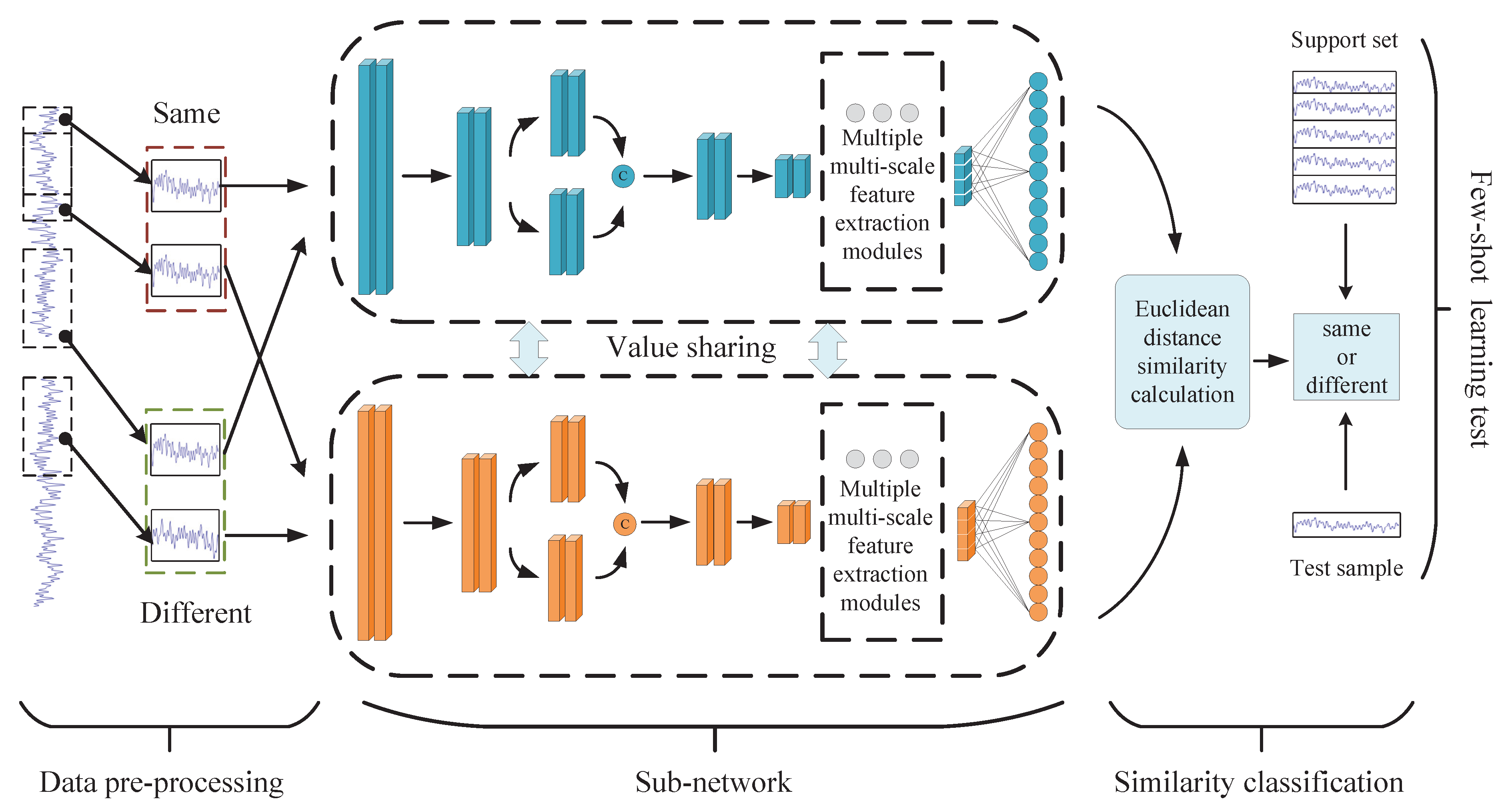
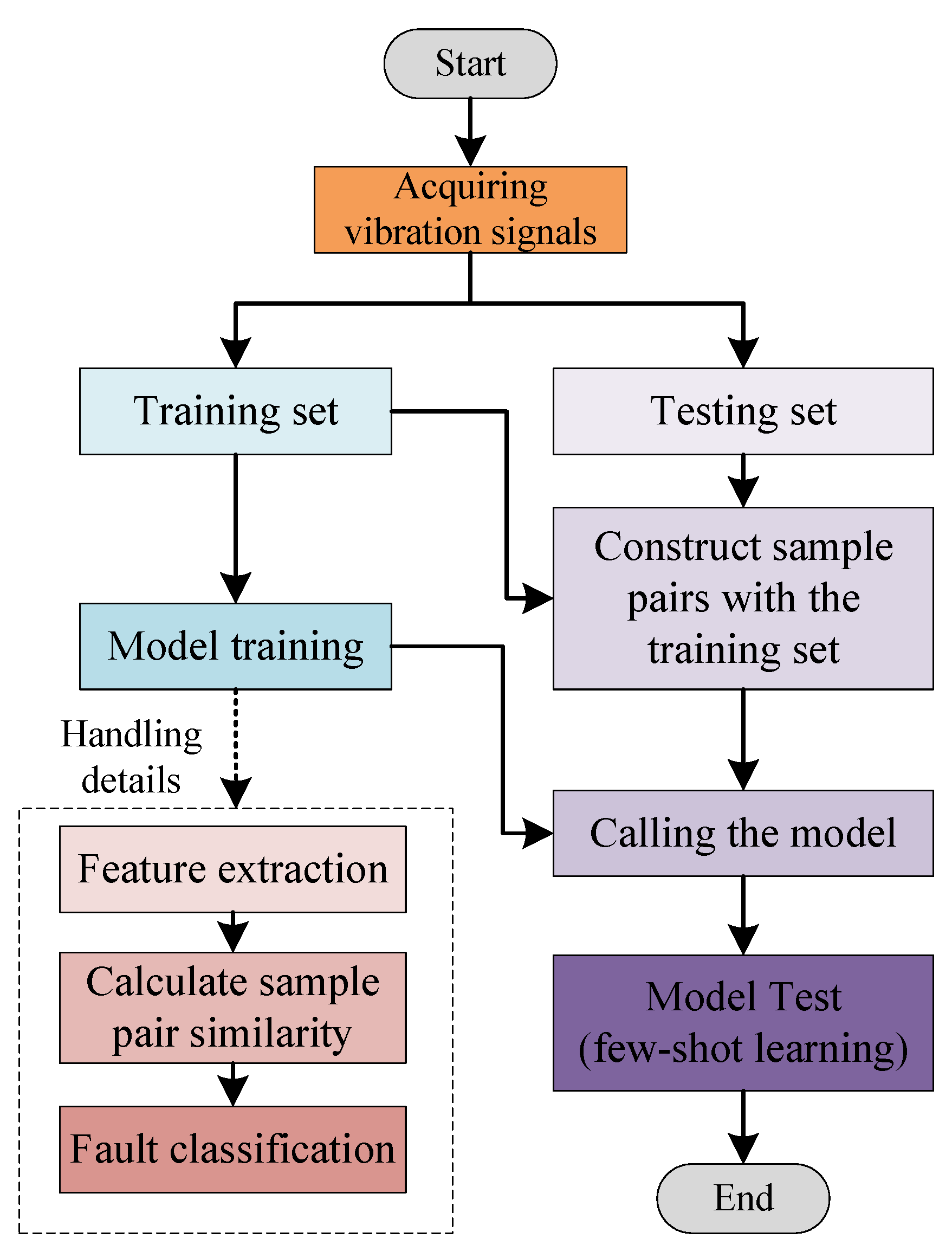
To overcome the problems of few samples and a huge amount of parameters, an end-to-end multi-scale and lightweight Siamese network with symmetrical architecture (MLS-net) is proposed in this paper. MLS-net not only maintains good accuracy in bearing fault diagnosis under small samples but also has fewer parameters to reduce resource consumption and a good generalization ability. The main contributions are summarized below.

• We construct a novel fault diagnosis network architecture by combining an improved Siamese network and few-shot learning for the case of small samples.
• A multi-scale feature extraction module is designed to improve the feature extraction capability of the model. Furthermore, we use the dimensionality reduction method to compress the parameters of the model to conserve device resources.
• Extensive experiments are conducted on multiple datasets to demonstrate the efficiency and generalization of the proposed architecture.

The rest of the paper is organized as follows: Section 2 introduces the mentioned basic theory. Section 3 describes the proposed network structure. Section 4 presents the details and results of the experiments. Section 5 concludes the paper.

2. Preliminaries

2.1. Inception

The inception module has an important role in model compression and feature extraction [26]. The key to the module improvement is the introduction of 1 × 1 convolution and the construction of a multi-scale convolution structure. The accuracy of the model on image classification was proven to be significantly improved through experiments. In addition, the model can utilize the computational resources more efficiently. More features are acquired with the same amount of parameters. The accuracy is also significantly improved. At the same time, the problems of overfit, gradient explosion and gradient disappearance due to the increased depth of the model are also improved.

There are four branches in the inception module. The first three branches use 1 × 1 convolution kernels for dimensionality reduction, which serves to optimize the problem of too many parameters caused by convolution operations. The reduction in dimensionality also brings a reduction in calculations. It is beneficial to the full utilization of computational resources. In addition, convolution kernels with different sizes are used to obtain different perceptual fields in the inception module. The branch contains 1 × 1, 3 × 3 and 5 × 5 sizes.

The different sizes of the convolution kernels allow for richer information to be extracted from the features. At the same time, multi-scale convolution uses the principle of decomposing sparse matrices into dense matrices to speed up the convergence. A comparison of the traditional convolution and inception modules is shown in Figure 1.

2.2. Siamese Network

A Siamese network [27] is a symmetrical architecture built from two neural networks. They are mainly applied in small sample cases. The inputs of the model are two samples from the same or different datasets. The main body consists of feature extraction and a similarity calculation module. The function of the feature extraction module outputs the feature vectors of the input samples. The similarity calculation module calculates the similarity of the two feature vectors. The similarity is compared between the predicted data and the prior knowledge using the model obtained from training. Thus, fault classification with small samples is achieved. Its emergence solves the problem of deep neural networks to obtain high accuracy and overfitting in the absence of a large number of data samples.

2.3. Few-Shot Learning

Few-shot learning [28] is the use of few samples for classification or regression. It is different from traditional supervised learning methods. Few-shot learning does not generalize the training set to the test set. It aims to make the model understand the similarities and differences of things and learn to distinguish between different things.

Few-shot learning generally consists of a support set (S), a query set (Q), a training set (T) and a judgment rule (R), where S contains a small amount of supervised information in Q. The combination of S and Q is used for predictive classification. R is the procedure equipped to determine the similarities and differences of things. We use T as prior knowledge to train R. R is then used to determine the similarities and differences between samples in S and Q to achieve small sample classification.

3. Methodology

3.1. Structure of MLS-Net

The overall architecture of MLS-net is shown in Figure 2. We fuse the improved sub-network with a Siamese network. A multi-scale and lightweight bearing fault diagnosis architecture applied to the small sample situation is constructed. The whole structure body consists of two symmetrical branches. As we can see from the figure, the overall architecture contains four parts: data pre-processing, the sub-network, similarity classification and the few-shot learning test.

3.1.1. Data Pre-Processing

The data pre-processing part focuses on the construction of the dataset that needs to be input into the model. The intercepted fault data from the same class and different classes are randomly combined to form the same and different class sample pairs. In the input sample pairs, we input the bearing vibration data from the sample pairs into the two symmetrical feature extraction branches separately.

The whole network needs to input pairs of samples in the format ($x_1$, $x_2$, $\mathcal{Y}$). Each sample pair contains a label $\mathcal{Y}$. When $\mathcal{Y}$ is 1, it means that the input sample pairs are fault data of the same category. However, when $\mathcal{Y}$ is 0, it means that the input sample pairs are the fault data of different categories. The corresponding $x_1$ and $x_2$ represent the two vibration data to be input. Further details of the data pre-processing can be found in Section 4.1.

3.1.2. Sub-Network

The sub-network part has two feature extraction modules with shared weights. The shared weights ensure that the results obtained from the two branches are comparable during similarity classification. The main purpose of this part is to extract the feature vector of the bearing fault data after convolutional processing using an optimized sub-network. The structure of the sub-network consists of multiple multi-scale and reduced dimensional feature extraction modules. The fused multi-scale feature information is used to enhance the model’s ability to obtain information from the samples. The function of the dimensionality reduction module is as a reducing parameter.

3.1.3. Similarity Classification

The similarity classification part mainly uses the distance formula to calculate the similarity between the feature vectors of the two branches. A similarity percentage is given after normalization. This similarity percentage is used to determine whether the two input bearing fault vibration data are of the same class. We use the trained similarity calculation model in combination with the few-shot learning test method to realize bearing fault diagnosis.

To implement the similarity calculation module, we first use the distance formula to obtain the distance between two feature vectors. The closer the two feature vectors are, the more likely that we can assume that they are the same class. When far apart, they are different classes. We chose the Euclidean distance as the metric formula for the two feature vectors. The formula is as follows.

$$s_t(x_1,x_2)=\left|\right|t\left(x_1\right)-t\left(x_2\right)\left|\right|$$

(1)

where $x_1$ and $x_2$ are the input samples. $t\left(x_1\right)$ and $t\left(x_2\right)$ are the feature vectors obtained after sub-network processing. $s_T(x_1,x_2)$ is the Euclidean distance.

The output of the entire network indicates the similarity of the sample pairs. In fact, this problem has been transformed into a binary classification problem in the similarity classification module. This is to give a probability to determine whether two input samples are of the same class or different classes. We use the sigmoid function to map the distance between two feature vectors to the range of (0, 1). The probability is used to intuitively predict the magnitude of the distance between the two vectors. The formula to calculate the output is as follows.

$$p(x_1,x_2)=sigm\left(FC\left(s_T(x_1,x_2)\right)\right)$$

(2)

where $FC$ is full connection processing for Euclidean distance output. $sigm$ is sigmoid function. $p(x_1,x_2)$ is the probability of the similarity of sample pairs.

As the whole similarity calculation module is transformed into a binary classification problem. When the entire network is trained, binary cross entropy is used as the loss function of the network. The corresponding formula is as follows:

$$\begin{array}{cc}& Loss=-\mathcal{Y}(x_1,x_2)log\left(p(x_1,x_2)\right)+(1-\mathcal{Y}(x_1,x_2))log(1-p(x_1,x_2))\hfill \end{array}$$

(3)

where $\mathcal{Y}$($x_1$, $x_2$) represents the corresponding label. The same is “1”, and different is “0”.

Once the loss function is determined, a gradient descent function can be used to train the Siamese network. The model weights are fine-tuned over multiple cycles by using forward and backward propagation. A network model that can determine the similarity of the fault samples is trained. We can use the trained similarity classification model and few-shot learning test method for bearing fault diagnosis.

3.1.4. Few-Shot Learning Testing

The C-shot K-way testing is generally used to test the model under the situation of small samples. K classes are extracted from the existing dataset, and C samples from each class are taken to build the support set as the test criteria. The test set is called the query set. We use the similarity classification module to calculate the similarity probability between the support set and the query set. With the help of the similarity probability, we can easily determine the category of the test sample. The general testing methods include one-shot K-way testing and C-shot K-way testing.

In one-shot K-way testing, each class in the support set S contains only one sample. This test aims to calculate the probability of similarity for each sample pair consisting of a support set and a query set. The sample pairs with the highest probability are of the same kind. The definition of S and the formula for the highest score T are as follows.

$$S=\left\{(x_i,y_i)|i=1,2...K\right\}$$

(4)

$$T(\widehat{x},S)=argmax\left(P(\widehat{x},x_k)\right),x_k\in S$$

(5)

In the C-shot K-way testing, each class in the support set S contains only C samples. Unlike one-shot K-way testing, this is performed by comparing the maximum of the sum of the probability. The specific formula is as follows.

$$S_C=\left\{\left(S_i\right|i=1,2...C)\right\}$$

(6)

$$T(\widehat{x},S_C)=argmax\left\{\sum _{i=1}^{n}P(\widehat{x},x_{C}k)\right\},x_{C}k\in S_C$$

(7)

3.2. Sub-Net Optimization

Siamese networks have been proven to be effective in dealing with small sample size problems. However, when the structure of feature extraction network is simple. The model cannot effectively extract enough features from the samples for classification. This article improves on the branches in the Siamese network to overcome the above problem. The sub-network is improved to a multi-scale and lightweight structure. The model extracts rich features through convolution kernels of different sizes. We use 1 × 1 convolution kernels to compress the model and reduce the calculations. This method can improve the model feature extraction capability and model accuracy. The optimization of sub-network module is shown in Figure 3.

The optimization for sub-network module is mainly inspired by the Inception module. The improvement of the sub-network is based on a convolutional network with a first layer of wide convolution [29]. As shown in Figure 3, the new model retains the wide convolutional layer of the first layer in the original network. This is to extract more feature information from the one-dimensional bearing vibration data, while other layers introduce multi-scale modules and 1 × 1 for sub-network optimization. The 3 × 3 and 5 × 5 convolution kernels generate a huge amount of computation when there are too many parameters in the input. We introduce a 1 × 1 convolution kernel to achieve dimensionality reduction of the data, thus, reducing the amount of calculation and model parameters.

After the model is processed by the first layer of wide convolution, it continues to be processed by the multi-scale module to obtain richer feature information. The multi-scale module can have different perceptual fields compared to the conventional convolution module. There are two types of multi-scale convolution modules in the model. One is a combination of 3 × 3 convolution and 5 × 5 convolution named IncConv1. The other is the combination of 1 × 1 convolution and 3 × 3 convolution named IncConv2. Due to the larger scale of the data in the first stage. The IncConv1 is chosen for processing in the model. As the scale of the processed data decreases and the depth of the model increases, the IncConv2 is gradually chosen for processing. This is to reduce the parameters and computational effort.

The parameters of the convolutional layers in the sub-network are as follows: the input part is 2048 × 1 size data. The size of the convolutional layer in the first layer is 64 × 1 and contains a total of 16 convolutional kernels. The step size of the convolutional layers after this one is 1. The size of the second layer is 5 × 1 and contains 32 convolutional kernels. The third layer is the IncConv1 module mentioned above. It is a combination of convolutional kernels of sizes 3 × 3 and 5 × 5. The fourth and fifth convolutional layers are the IncConv1 modules. These are a combination of 1 × 1 and 3 × 3 size convolutional kernels.

Before the fully connected layer is a dropout layer with a parameter set to 0.5. It is used to prevent overfitting during model training and to accelerate the convergence of the model. The final output is a fully-connected layer with an output of 100. We add a maximum pooling layer after each convolutional layer. The size of each maximum pooling layer is 2 × 1, and the stride is 1. The maximum pooling is to reduce the model parameters and increase the computational speed while extracting features robustly.

3.3. Processing of the Network

The specific operations can be seen in Figure 4 in the following modules.

• Preprocessing: The bearing fault vibration data is segmented using sliding windows to obtain the bearing fault samples. We construct a training set and a test set according to the requirement that the model input is a sample pair.
• Model training: The training set is divided into sample pairs with equal proportions of the same and different classes of faults. We feed the training samples into the network. Then, the network is trained by using the Adam gradient descent algorithm and a binary cross entropy loss function. Finally, we save the model with the best training results.
• Model testing: We first combine the samples from the test set and the training set in order to form a support set. The trained optimal model is used in the similarity probability calculation. The sample pair with the highest similarity probability among the obtained multiple similarities is selected as the fault class.

4. Experimentation and Analysis

4.1. Data Set Preparation

We must understand the performance of the proposed network structure in the case of insufficient samples. Three datasets are used for validation in this experiment. They are the Case Western Reserve University (CWRU) bearing fault dataset [30], Mechanical fault Prevention Technology Institute (MFPT) bearing fault dataset [31] and Laboratory simulated bearing fault dataset.

(1) CWRU bearing fault dataset

For this experiment, the 12 kHz bearing fault on the drive side from the Case Western Reserve University bearing dataset is used as the experimental data. The fault types are divided into four categories: normal, ball fault, inner ring fault and outer ring fault. Each fault, in turn, contains three fault categories of 0.007, 0.014 and 0.021 inch dimensions; therefore, the total number of fault categories is 10. The specific classification is in

Table 1. CWRU bearing dataset classification description.

Fault Location (inch)	Status Labels	Number of Training Samples	Number of Test Samples
Normal	0	1980	75
Rolling ball (0.007)	1	1980	75
Rolling ball (0.014)	2	1980	75
Rolling ball (0.021)	3	1980	75
Inner race (0.007)	4	1980	75
Inner race (0.014)	5	1980	75
Inner race (0.021)	6	1980	75
Out race (0.021)	7	1980	75
Out race (0.021)	8	1980	75
Out race (0.021)	9	1980	75

.

(2) MFPT bearing fault dataset

The MFPT dataset is provided by the Mechanical Prevention Technology Association. The dataset contains data from the experimental bench and three real-world fault data. Fault types are divided into three categories: baseline conditions, outer race fault conditions and inner race fault conditions. The sampling frequency of the data set is 25 Hz. We selected seven types of data from MFPT to construct the experimental dataset. The fault types are classified into three categories: normal, outer ring fault and inner ring fault. Each fault class data is selected with load conditions of 50, 200 and 300 lbs. The total number of classes of the fault categories in the experimental dataset is seven. The specific classification is in

Table 2. MFPT bearing dataset classification description.

Fault Location (lbs)	Status Labels	Number of Training Samples	Number of Test Samples
normal	0	660	25
Out race (50)	1	660	25
Out race (200)	2	660	25
Out race (300)	3	660	25
Inner race (50)	4	660	25
Inner race (200)	5	660	25
Inner race (300)	6	660	25

.

(3) Laboratory bearing fault dataset

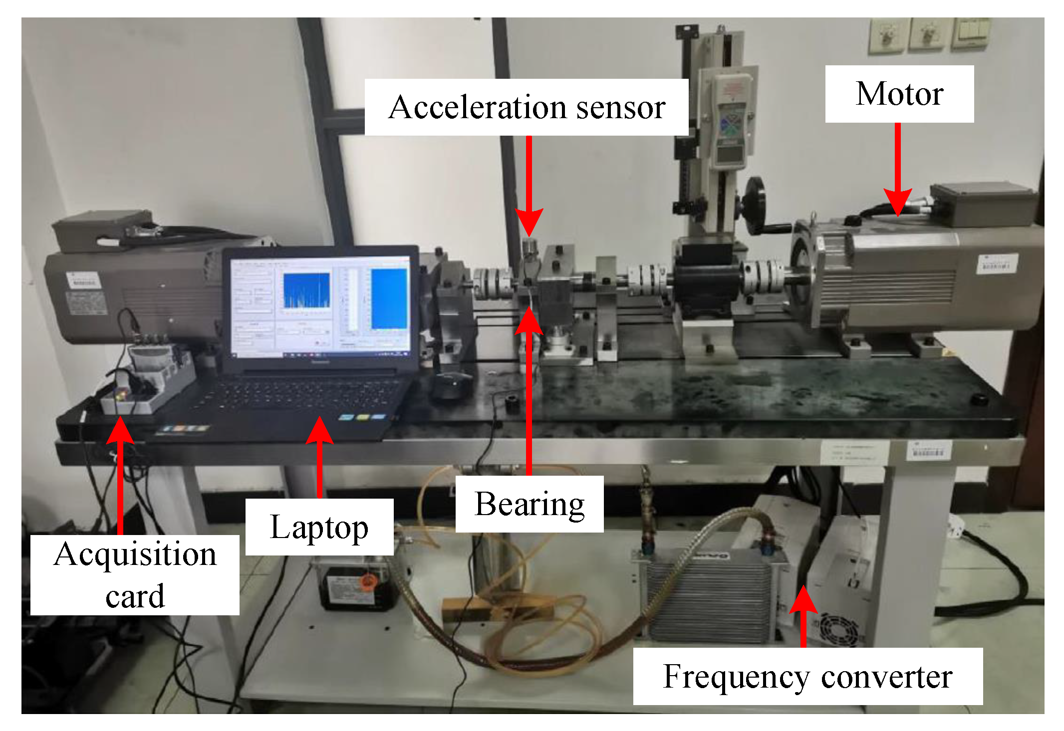
The main structure of the test bench is shown in the diagram below. The components are the following: accelerometer, bearings, motors, acquisition cards, frequency converter and external computers and other key devices. The positions of the individual devices are marked in Figure 5. The entire experimental equipment is rotated by motors driving the bearing parts. The accelerometers collect the vibration signal in real time. The vibration signal is then transferred to the computer for storage and analysis by means of an acquisition card.

The experiments conducted in this case are set up for three fault situations. The faults are outer race fault, inner race fault and ball fault. All three faults are set as scratch faults. Three faults are set to penetrate in the axial. The width of the fault is 1.2 mm, and the depth is 0.5 mm. All three faults are tested twice at 1800 and 3000 r/min, respectively. Therefore, all fault categories are divided into six categories. Details of the corresponding health conditions are shown in the following

Table 3. Laboratory bearing dataset classification description.

Fault Location (r/min)	Status Labels	Number of Training Samples	Number of Test Samples
Out race (1800)	0	660	25
Out race (3000)	1	660	25
Inner race (1800)	2	660	25
Inner race (3000)	3	660	25
Rolling ball (1800)	4	660	25
Rolling ball (3000)	5	660	25

.

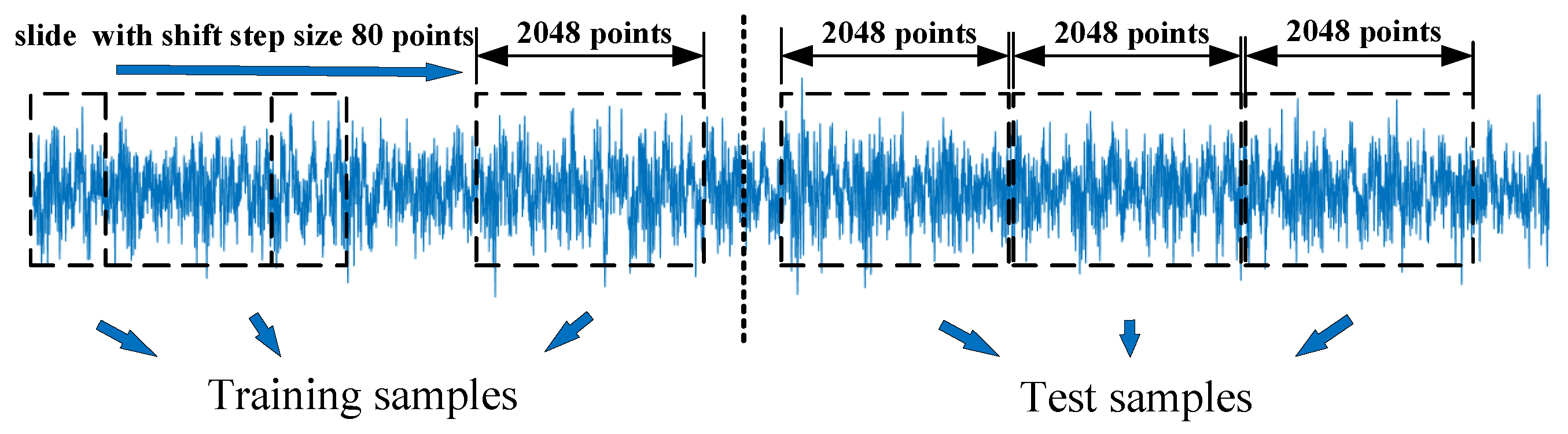
Each type of fault data is a vibration signal collected by an accelerometer. To ensure consistent conditions with the comparison schemes, the dataset is constructed based on the method in [29]. The detailed schematic diagram for building the training and test sets is shown in Figure 6. We build the training set from the first half of the vibration signal and the test set from the second. Each training sample is 2048 points in length. We use a sliding window with a step size of 80 to intercept the training samples sequentially backwards. The data intercepted by the sliding window is the training set. The second half of the vibration signal is divided into multiple non-overlapping test samples, and each test sample also contains 2048 points.

4.2. Experimental Setup

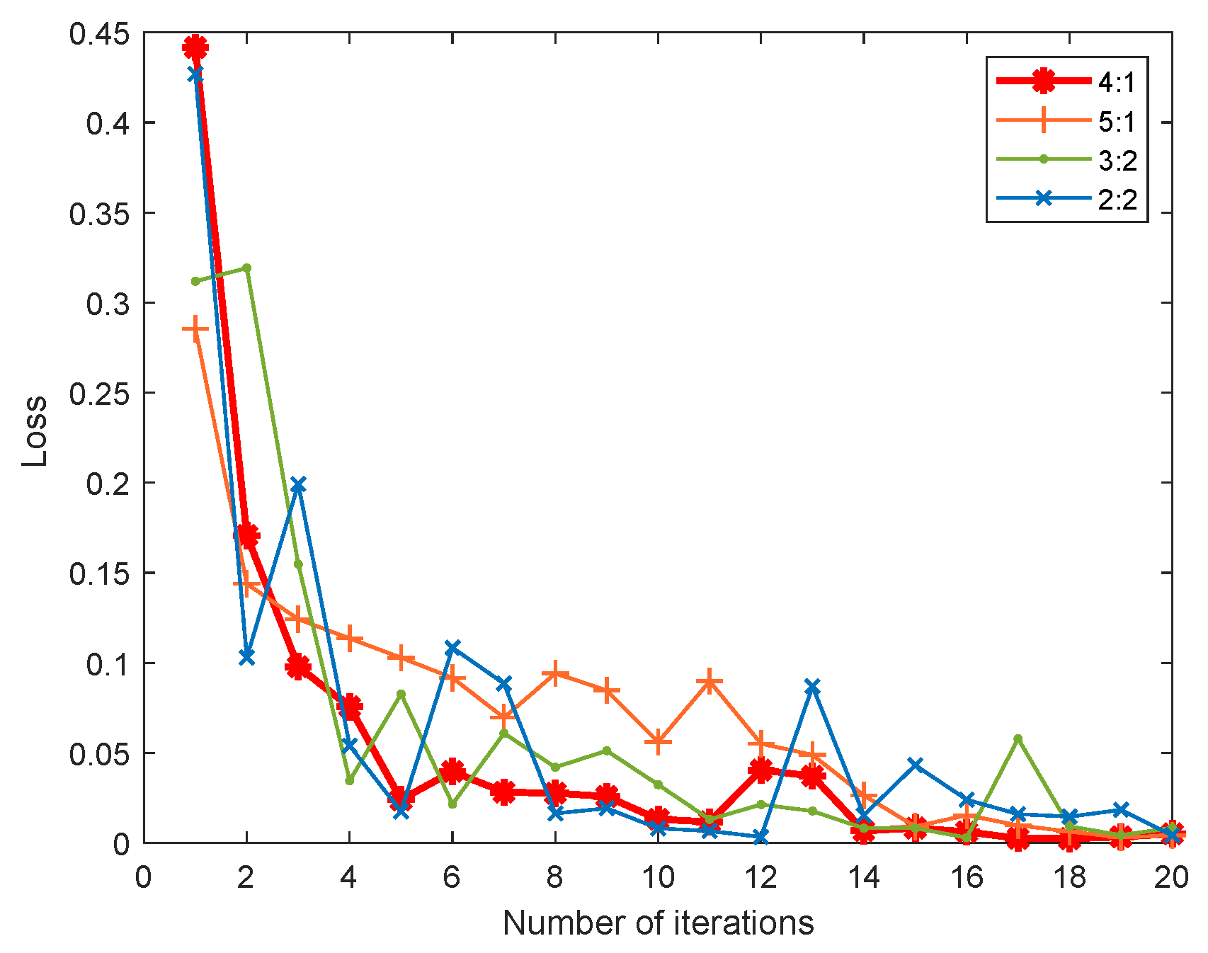
The training samples are divided into the training set and validation set. By comparing the loss rate under different ratios in Figure 7, the ratio of the training set and validation set is configured to be 4:1 for better convergence performance. In addition, the model is implemented using the Keras library and Python 3.6. The total epoch of model training is 15,000, and the small batch size is 32. The optimal model is saved after 20 training sessions have been conducted in the experiment.

To validate the performance of the models obtained by training under different samples, the quantities 60, 90, 120, 200, 300, 600 and 900 are randomly selected on the CWRU and Laboratory datasets. The number of fault types selected in MFPT is seven. For the sake of balance of the training data, we randomly select the quantities 70, 105, 140, 210, 280, 490 and 700.

The sample pairs we input each time are randomly selected from the above training set. When they belong to the same class, they are labeled as positive samples; otherwise, they are negative samples. We also need to ensure that the number of positive and negative sample pairs is equal to ensure a balanced sample.

In Experiment 1, we vary the number of multi-scale modules in the model to determine the optimal model structure. In Experiment 2, we test the model on three datasets to verify the performance of MLS-net. In Experiment 3, we visualize the model performance using visualization tools. In Experiment 4, we calculate the model size and parameters.

The following three methods will be tested on the three datasets to compare with the new proposed model.

• Support Vector Machine (SVM): SVM is a classical machine learning method for dichotomous classification problems. We use an SVM between any two classes to implement a multi-classification task.
• One-Dimensional Convolutional Neural Network (1D-CNN) [29]: 1D-CNN, which is a five-layer DCNN. It uses 64 × 1 convolutional kernels for the first layer and 3 × 1 convolutional kernels for the next four layers. The corresponding number of convolutional kernels is 16, 32, 64, 64 and 64. We add a maximum pooling layer of size 2 × 1 after each convolutional layer. The final layer is a fully connected layer with an output of 100.
• The baseline Siamese network (BS-net) [32]: BS-net has the same structure as the proposed Siamese network. However, the structure of sub-network in the Siamese network is the 1D-CNN mentioned above.

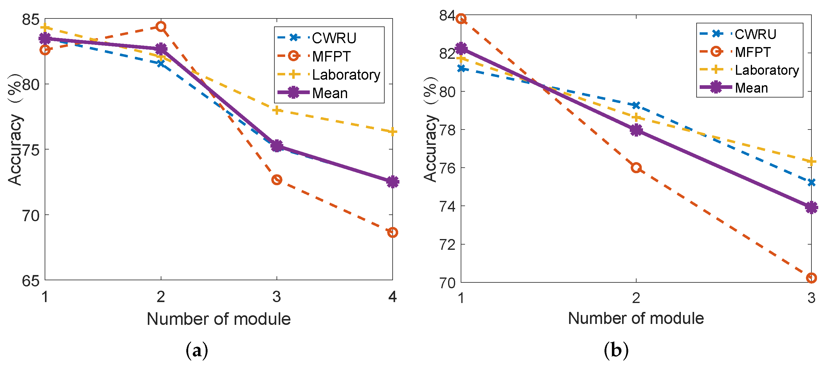
4.3. Determination of the Number of Multi-Size Modules

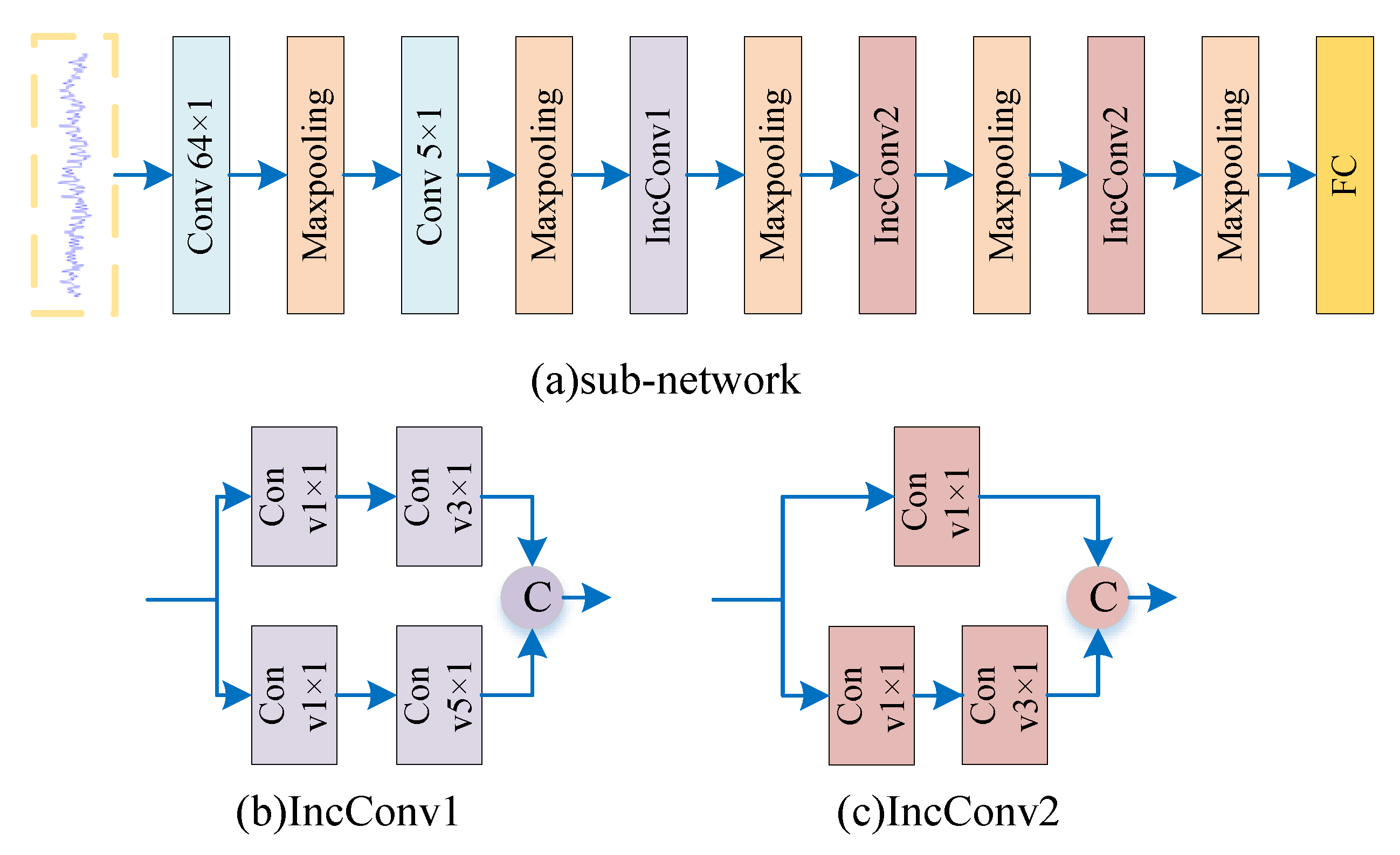
We want to determine the optimal number of multi-size modules in the model. The multi-size modules are divided into two categories by the introduction of the sub-network. The larger size is a fusion of 5 × 5 and 3 × 3, which we call IncConv1. The smaller size is a fusion of 3 × 3 and 1 × 1, which we call IncConv2. Under the premise that the sample size is set to 60, we will vary the number of these two modules to determine the optimal number of modules.

The comparison between

Table 4. Comparison of IncConv2 numbers (number of IncConv1 is 1).

IncConv2 Numbers	Datasets	Accuracy (%)	Mean (%)	Total Number of Parameters
1	CWRU	83.50	83.47	63,897
	MFPT	82.60
	Laboratory	84.32
2	CWRU	81.55	82.67	41,449
	MFPT	84.39
	Laboratory	82.08
3	CWRU	75.12	75.26	31,801
	MFPT	72.67
	Laboratory	78.00
4	CWRU	72.56	72.51	28,452
	MFPT	68.64
	Laboratory	76.34

and

Table 5. Comparison of IncConv2 numbers (number of IncConv1 is 2).

IncConv2 Numbers	Datasets	Accuracy (%)	Mean (%)	Total Number of Parameters
1	CWRU	81.21	82.25	43,497
	MFPT	83.83
	Laboratory	81.73
2	CWRU	79.26	77.96	33,849
	MFPT	76.00
	Laboratory	78.64
3	CWRU	75.23	73.92	30,601
	MFPT	70.23
	Laboratory	76.32

shows that the trend of the accuracy of the model decreases as the number of the IncConv1 increases. This shows that the number of modules for IncConv1 should be 1. Figure 8a,b shows the variation of accuracy on each data set and the mean of the three types of data. The mean lines in both plots show that, as the number of modules increases, the accuracy rate decreases. However, our previous analysis shows that the number of IncConv1 should be 1.

Therefore, we only need to observe Table 4 to determine the number of IncConv2. We find that the accuracy rate decreases as the number of modules increases.The accuracy of the models is similar at number 1 and 2; however, the total number of parameters is different. To balance the accuracy and the total number of parameters, we finally decided to set the number of IncConv2 to 2.

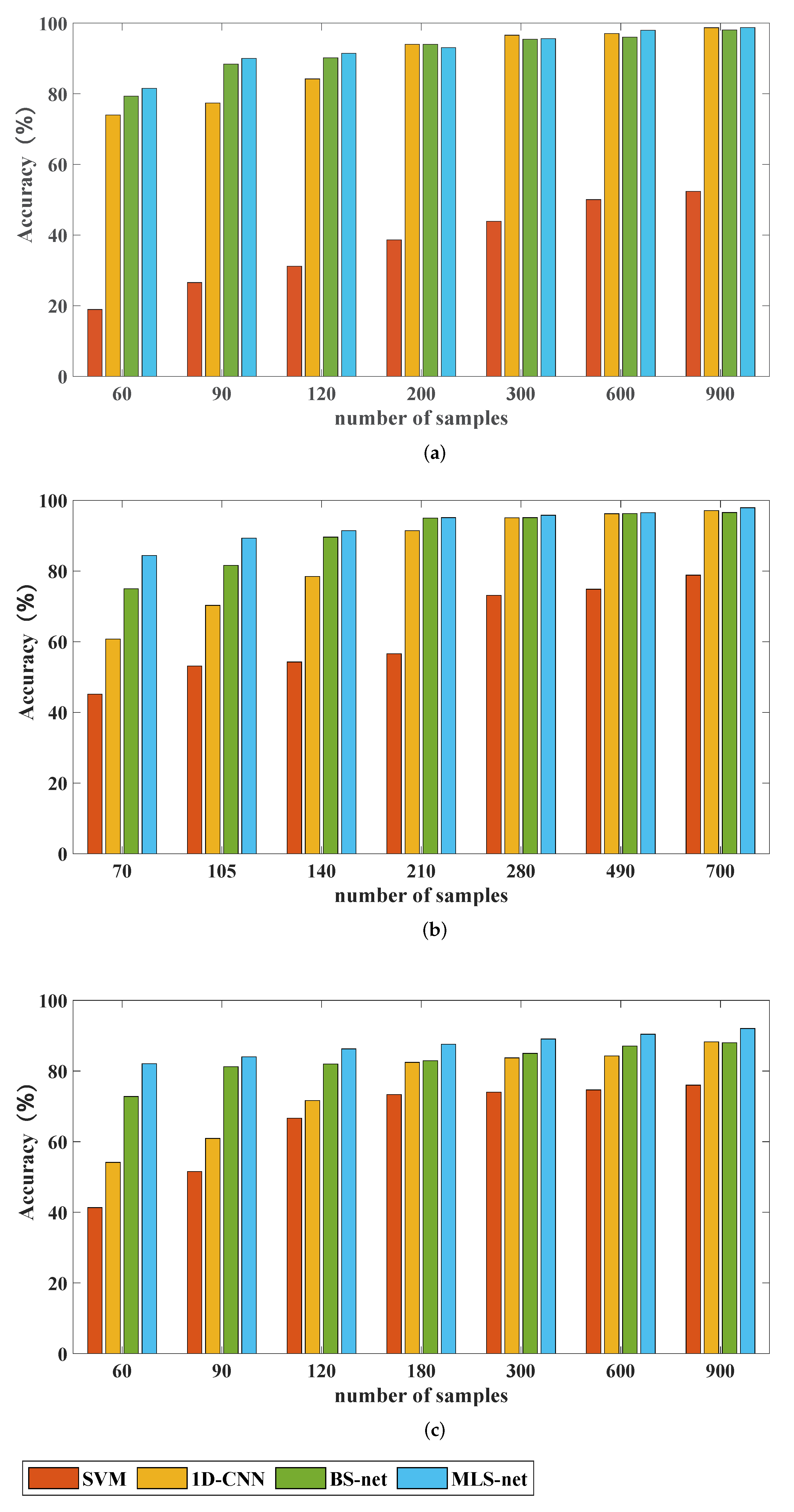
4.4. Model Effects with Different Sample Sizes

In this section, we want to verify that the proposed method performs well in the case of insufficient samples. We chose the methods described above: (SVM), 1D-CNN, BS-net and MLS-net for performance comparison. Several models are tested on three bearing fault datasets.

Table 6. Comparison of sample sizes.

Datasets	Models	Number of Samples
CWRU		60	90	120	200	300	600	900
	SVM	18.93	26.56	31.20	38.67	43.89	50.05	52.35
	1D-CNN	73.97	77.39	84.19	93.97	96.59	97.03	98.69
	BS-net	79.33	88.41	90.15	94.00	95.45	96.00	98.07
	ANS-net [22]	88.64	90.60	-	-	98.24	98.59	99.05
	MLS-net	81.55	90.02	91.44	93.04	95.59	97.97	98.74
MFPT		70	105	140	210	280	490	700
	SVM	45.14	53.14	54.26	56.57	73.14	74.85	78.85
	1D-CNN	60.76	70.28	78.47	91.42	95.09	96.23	97.13
	BS-net	74.97	81.6	89.6	94.97	95.12	96.25	96.57
	MLS-net	84.39	89.32	91.44	95.12	95.79	96.53	97.91
Laboratory		60	90	120	180	300	600	900
	SVM	41.33	51.53	66.66	73.33	74	74.66	76
	1D-CNN	54.13	60.93	71.66	82.46	83.73	84.26	88.26
	BS-net	72.80	81.20	82.00	82.93	85.00	87.06	88.00
	MLS-net	82.08	83.99	86.23	87.56	89.05	90.41	92.02

and Figure 9 show the results of the experiments.

It is clear that the MLS-net shows the most excellent results. We analyze the results of each dataset and see that the SVM method has a significant difference in accuracy compared to the other methods. The accuracy of the SVM differs from other methods by nearly 20% or more when the sample is insufficient. There is also a 10% difference in accuracy with a large number of samples. It can be seen that the deep-learning approach is far superior to SVM. Compared with 1D-CNN, the Siamese network model is more complex in structure. The model cleverly uses metrics for similarity calculation and incorporates few-shot learning methods.

This makes the ability of fault classification significantly better than 1D-CNN in the case of small samples. The MLS-net is compared with BS-net by experimental data. When the samples are insufficient, the accuracy of the MLS-net is improved in all cases. It can be seen that the introduced multi-size convolutional module can obtain richer information. With the increase of samples, the accuracy of both tends to be the same. Sometimes the accuracy of the old model is higher than that of the MLS-net. The difference between the two models is within 1%. It can be seen that there is minimal loss of accuracy when the sample is sufficient.

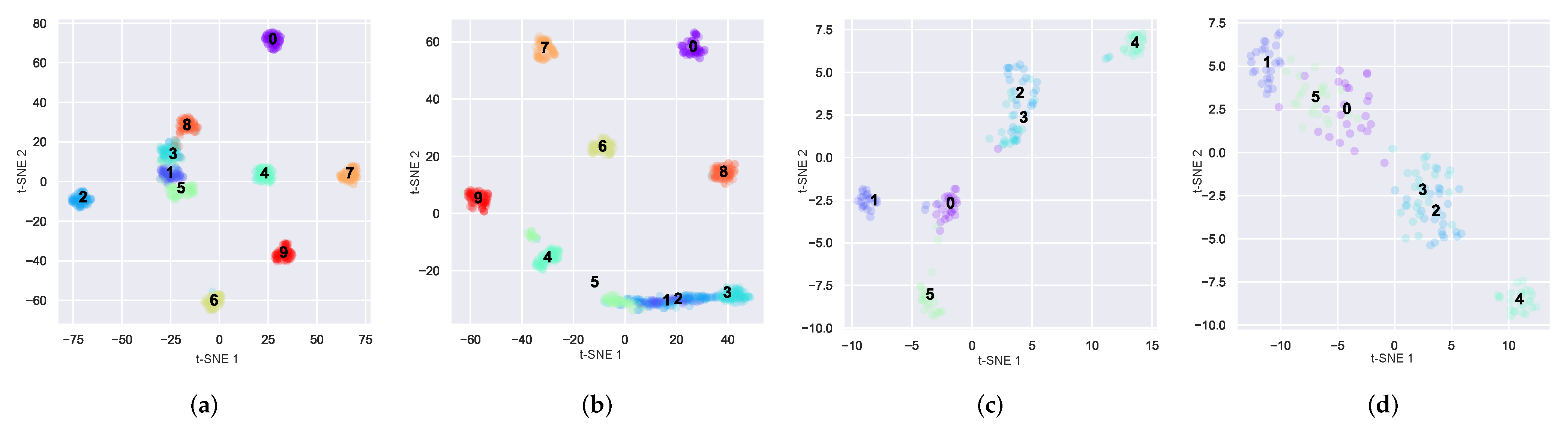
4.5. Visualization Analysis

We attempted to obtain a better understanding of how well the model performs in the presence of insufficient samples. We would like to make further proof by using the feature visualization method of t-SNE and the confusion matrix of the test results. In Figure 10, we show the visualization of the last layer of the fully connected layer on the CWRU dataset and Laboratory dataset. The number of samples for model training is set to 90. In Figure 11, the confusion matrix plot of the test results on these two datasets is also shown. The comparison methods used in both plots are the BS-net and the MLS-net proposed in this paper.

In Figure 10, the Figure 10a,b are of the CWRU dataset. Figure 10c,d are the Laboratory dataset. As can be seen in the figure on the CWRU dataset, the MLS-net can be clearly seen on categories 1, 2 and 3 with a good distinction. Whereas, on the BS-net it shows that the three categories are mixed together and cannot be clearly distinguished. It can be seen that the BS-net is not as good at classifying as the MLS-net. This problem is more apparent in the Laboratory data set. Multiple classes are mixed together and all data distribution is discrete on the BS-net. This problem is well resolved in the plots of the MLS-net. It can be seen that the MLS-net has a better ability to classify samples with small samples.

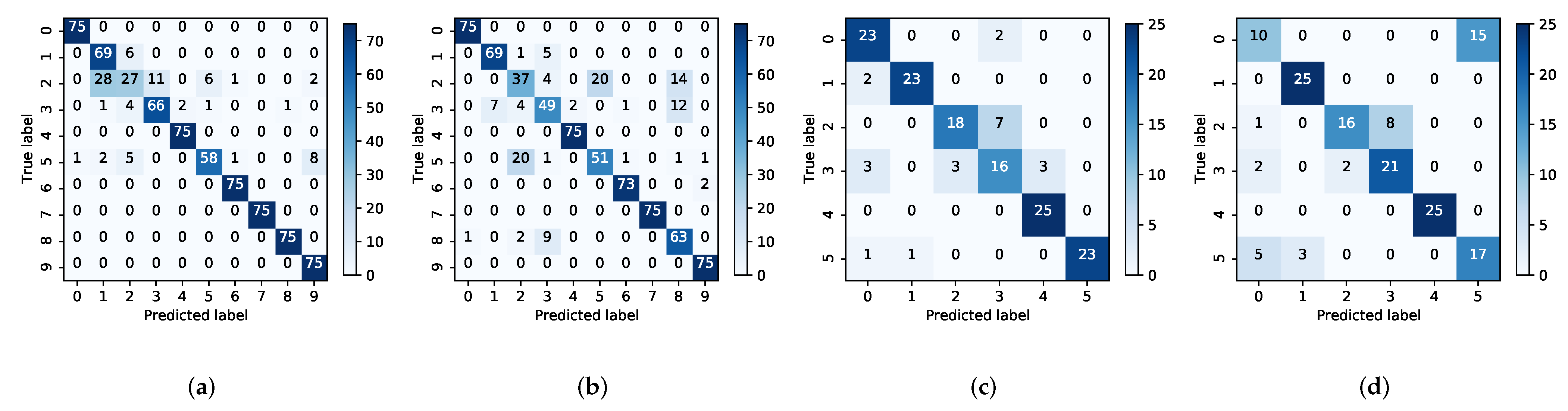
In Figure 11, Figure 11a,b are the CWRU bearing dataset and Figure 11c,d are the Laboratory bearing dataset. As we can see in both Figure 11a,b, the number of accurate judgements for each category in Figure 11a is greater. Whereas, in Figure 11b, it is clear that the accuracy of per category is much lower. In Figure 11c,d, the comparison of the two models is also the same. This shows that the new model also has a superior performance in prediction compared to the BS-net. At the same time, the performance of the MLS-net is consistent across the different dataset. It means that the MLS-net can be applied to practical bearing fault diagnosis.

4.6. Model Lightweight Comparison

In this subsection, the main purpose is to analyze the comparison of model size under different models and datasets. The results of the experiment mainly contain the total number of model parameters and model sizes for SVM, 1D-CNN, BS-net and MLS-net under the three dataset. The recently proposed bearing fault diagnosis models ANS-net [22] and LEFE-net [23] are also compared. We jointly determine the merit of a model based on the parameters and the accuracy rate. A model that has fewer parameters while having the higher accuracy will have superior performance. The system cost and the speed of computation will be greatly increased under fewer parameters. The details are shown in the following Figure 12 and

Table 7. Comparison of model parameters and sizes.

Models	Datasets	Total Number of Parameters	Model Size
SVM	CWRU	-	110,837 KB
	MFPT	-	108,460 KB
	Laboratory	-	108,460 KB
1D-CNN	CWRU	52,806	663 KB
	MFPT	52,503	660 KB
	Laboratory	52,402	659 KB
BS-net	CWRU	53,945	680 KB
	MFPT
	Laboratory
ANS-net	CWRU	>100,000	-
	MFPT
	Laboratory
MLS-net	CWRU	41,449	566 KB
	MFPT
	Laboratory
LEFE-net	CWRU	56,640	-

.

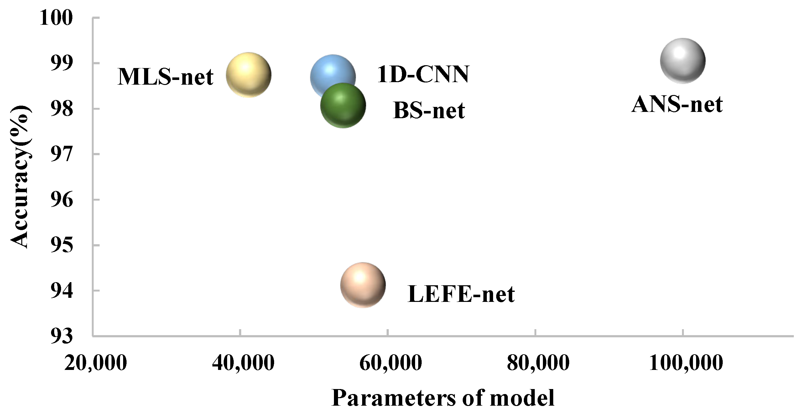
In Figure 12, we mainly depict the relationship between model accuracy and total number of parameters. The horizontal coordinate indicates the model parameters. The vertical coordinate indicates the accuracy rate. The accuracy of each model is obtained from the experiment when the sample size is set as 900 for the CWRU dataset. As we can see from Figure 12, MLS-net shows the better performance in terms of the model parameters and accuracy compared with 1D-CNN and BS-net.

Although ANS-net has similar accuracy with MLS-net, the number of MLS-net parameters is only 41449, which is greatly reduced. The ANS-net, on the other hand, has far more than 100,000 parameters. LEFE-net has fewer parameters than ANS-net. However, its accuracy is lower than ANS-net and MLS-net when the training sample size is 900. When the sample drops to 60, the accuracy of LEFE-net will be further greatly reduced. Overall, MLS-net is able to run efficiently with less computation cost as well as guaranteed accuracy.

From Table 6 and Table 7 and Figure 12, it is clear that MLS-net has a significant improvement in model size and accuracy. Specifically, SVM is 100-times larger than MLS-net in terms of model size, while its accuracy is only 50% of MLS-net under small samples. MLS-net is also more advantageous in terms of the parameters of the model. It compresses about 20% parameters in comparison with BS-net and 1D-CNN. However, MLS-net under small samples improves the accuracy compared to 1D-CNN with an improvement of 10–15% and improves the accuracy by about 2–5% compared with BS-net.

ANS-net was recently proposed as a bearing fault diagnosis model for the small sample case. Although it has a high accuracy rate under small samples, a large number of parameters (more than 100,000) are needed to ensure the accuracy. In addition, MLS-net performs better in accuracy and lightweight than the lightweight bearing fault diagnosis model LEFE-net. Through the above experiments, MLS-net is proven to have a lighter model structure and better accuracy under small samples, which can greatly improve the efficiency of bearing fault diagnosis.

5. Conclusions

In this paper, we proposed the MLS-net for the end-to-end bearing fault diagnosis problem. The model has a great ability to classify in the case of small samples. It also has a multi-scale feature fusion module to enable further feature information to be acquired. With dimensionality reduction, the model is also able to obtain comparable accuracy with fewer parameters. The model was mainly designed based on the idea of metrics. Two symmetrical sample feature extraction modules with shared parameters are contained. These are mainly used to extract the feature vectors of the two sample pairs of the input. The similarity calculation module is used to calculate the similarity of the two extracted feature vectors. Thus, the trained model has the ability to compare the similarity probability between the standard samples and predicted samples. This enables the classification of the bearing fault.

To better validate the proposed model MLS-net, we tested it on three datasets to demonstrate its performance. The results show that the model had higher accuracy with fewer parameters when the sample was insufficient compared to recently proposed methods. This proves that MLS-net as proposed in our paper makes a good tradeoff between the accuracy and computing cost. In addition, the results were consistent across the three datasets tested. This indicates that the whole model has good generalization ability for different fault datasets.

The model showed good performance by retraining the method in this paper on multiple datasets. However, the need of retraining the model each time makes the operation cumbersome. In future work, we can focus our research more on the transfer scenarios of the model and fault diagnosis in noisy environments.

References

1. Wei, Y.; Li, Y.; Xu, M.; Huang, W. A review of early fault diagnosis approaches and their applications in rotating machinery. Entropy 2019, 21, 409. [Google Scholar] [CrossRef] [PubMed] [Green Version]
2. Zhang, S.; Zhang, S.; Wang, B.; Habetler, T.G. Deep learning algorithms for bearing fault diagnostics—A comprehensive review. IEEE Access 2020, 8, 29857–29881. [Google Scholar] [CrossRef]
3. Mohammed, S.A.; Ghazaly, N.M.; Abdo, J. Fault Diagnosis of Crack on Gearbox Using Vibration-Based Approaches. Symmetry 2022, 14, 417. [Google Scholar] [CrossRef]
4. Sikder, N.; Bhakta, K.; Al Nahid, A.; Islam, M.M. Fault diagnosis of motor bearing using ensemble learning algorithm with FFT-based preprocessing. In Proceedings of the 2019 International Conference on Robotics, Electrical and Signal Processing Techniques (ICREST), Dhaka, Bangladesh, 10–12 January 2019; pp. 564–569. [Google Scholar]
5. Zhang, K.; Ma, C.; Xu, Y.; Chen, P.; Du, J. Feature extraction method based on adaptive and concise empirical wavelet transform and its applications in bearing fault diagnosis. Measurement 2021, 172, 108976. [Google Scholar] [CrossRef]
6. Cheng, Y.; Wang, Z.; Chen, B.; Zhang, W.; Huang, G. An improved complementary ensemble empirical mode decomposition with adaptive noise and its application to rolling element bearing fault diagnosis. ISA Trans. 2019, 91, 218–234. [Google Scholar] [CrossRef] [PubMed]
7. Yu, G. A concentrated time–frequency analysis tool for bearing fault diagnosis. IEEE Trans. Instrum. Meas. 2019, 69, 371–381. [Google Scholar] [CrossRef]
8. Quinde, I.R.; Sumba, J.C.; Ochoa, L.E.; Morales-Menendez, R. Bearing fault diagnosis based on optimal time-frequency representation method. IFAC-Pap. 2019, 52, 194–199. [Google Scholar] [CrossRef]
9. Elbouchikhi, E.; Choqueuse, V.; Amirat, Y.; Benbouzid, M.E.H.; Turri, S. An efficient Hilbert–Huang transform-based bearing faults detection in induction machines. IEEE Trans. Energy Convers. 2017, 32, 401–413. [Google Scholar] [CrossRef]
10. Qian, S.; Yang, X.; Huang, J.; Zhang, H. Application of new training method combined with feedforward artificial neural network for rolling bearing fault diagnosis. In Proceedings of the 2016 23rd International Conference on Mechatronics and Machine Vision in Practice (M2VIP), Nanjing, China, 28–30 November 2016; pp. 1–6. [Google Scholar]
11. Xue, X.; Zhou, J. A hybrid fault diagnosis approach based on mixed-domain state features for rotating machinery. ISA Trans. 2017, 66, 284–295. [Google Scholar] [CrossRef]
12. Wang, T.; Liu, Z.; Lu, G.; Liu, J. Temporal-spatio graph based spectrum analysis for bearing fault detection and diagnosis. IEEE Trans. Ind. Electron. 2020, 68, 2598–2607. [Google Scholar] [CrossRef]
13. Goyal, D.; Choudhary, A.; Pabla, B.; Dhami, S. Support vector machines based non-contact fault diagnosis system for bearings. J. Intell. Manuf. 2020, 31, 1275–1289. [Google Scholar] [CrossRef]
14. Wang, X.; Mao, D.; Li, X. Bearing fault diagnosis based on vibro-acoustic data fusion and 1D-CNN network. Measurement 2021, 173, 108518. [Google Scholar] [CrossRef]
15. Hsueh, Y.M.; Ittangihal, V.R.; Wu, W.B.; Chang, H.C.; Kuo, C.C. Fault diagnosis system for induction motors by CNN using empirical wavelet transform. Symmetry 2019, 11, 1212. [Google Scholar] [CrossRef] [Green Version]
16. Chen, X.; Zhang, B.; Gao, D. Bearing fault diagnosis base on multi-scale CNN and LSTM model. J. Intell. Manuf. 2021, 32, 971–987. [Google Scholar] [CrossRef]
17. Goodfellow, I.; Pouget-Abadie, J.; Mirza, M.; Xu, B.; Warde-Farley, D.; Ozair, S.; Courville, A.; Bengio, Y. Generative adversarial nets. arXiv 2014, arXiv:1406.2661. [Google Scholar]
18. Xia, M.; Li, T.; Xu, L.; Liu, L.; De Silva, C.W. Fault diagnosis for rotating machinery using multiple sensors and convolutional neural networks. IEEE/ASME Trans. Mechatron. 2017, 23, 101–110. [Google Scholar] [CrossRef]
19. Wang, R.; Jiang, H.; Li, X.; Liu, S. A reinforcement neural architecture search method for rolling bearing fault diagnosis. Measurement 2020, 154, 107417. [Google Scholar] [CrossRef]
20. Sung, F.; Yang, Y.; Zhang, L.; Xiang, T.; Torr, P.H.; Hospedales, T.M. Learning to compare: Relation network for few-shot learning. In Proceedings of the IEEE conference on computer vision and pattern recognition, Salt Lake City, UT, USA, 18–23 June 2018; pp. 1199–1208. [Google Scholar]
21. Snell, J.; Swersky, K.; Zemel, R.S. Prototypical networks for few-shot learning. arXiv 2017, arXiv:1703.05175. [Google Scholar]
22. Fang, Q.; Wu, D. ANS-net: Anti-noise Siamese network for bearing fault diagnosis with a few data. Nonlinear Dyn. 2021, 104, 2497–2514. [Google Scholar] [CrossRef]
23. Fang, H.; Deng, J.; Zhao, B.; Shi, Y.; Zhou, J.; Shao, S. LEFE-Net: A lightweight efficient feature extraction network with strong robustness for bearing fault diagnosis. IEEE Trans. Instrum. Meas. 2021, 70, 1–11. [Google Scholar] [CrossRef]
24. Xiong, S.; Zhou, H.; He, S.; Zhang, L.; Shi, T. Fault diagnosis of a rolling bearing based on the wavelet packet transform and a deep residual network with lightweight multi-branch structure. Meas. Sci. Technol. 2021, 32, 085106. [Google Scholar] [CrossRef]
25. Zhang, S.; Ye, F.; Wang, B.; Habetler, T.G. Few-Shot Bearing Fault Diagnosis Based on Model-Agnostic Meta-Learning. IEEE Trans. Ind. Appl. 2021, 57, 4754–4764. [Google Scholar] [CrossRef]
26. Szegedy, C.; Liu, W.; Jia, Y.; Sermanet, P.; Reed, S.; Anguelov, D.; Erhan, D.; Vanhoucke, V.; Rabinovich, A. Going deeper with convolutions. In Proceedings of the IEEE Conference on Computer Vision and Pattern Recognition, Boston, MA, USA, 7–12 June 2015; pp. 1–9. [Google Scholar]
27. Chicco, D. Siamese neural networks: An overview. Artif. Neural Netw. 2021, 2190, 73–94. [Google Scholar] [CrossRef]
28. Wang, Y.; Yao, Q.; Kwok, J.T.; Ni, L.M. Generalizing from a few examples: A survey on few-shot learning. ACM Comput. Surv. 2020, 53, 1–34. [Google Scholar] [CrossRef]
29. Zhang, W.; Peng, G.; Li, C.; Chen, Y.; Zhang, Z. A new deep learning model for fault diagnosis with good anti-noise and domain adaptation ability on raw vibration signals. Sensors 2017, 17, 425. [Google Scholar] [CrossRef]
30. Loparo, K. Case western reserve university bearing data center. In Bearings Vibration Data Sets; Case Western Reserve University: Cleveland, OH, USA, 2012; pp. 22–28. Available online: https://engineering.case.edu/bearingdatacenter/download-data-file (accessed on 1 October 2021).
31. Dataset, M. Society for Machinery Failure Prevention Technology. 2012. Available online: https://www.mfpt.org/exhibitor-info/proceedings/ (accessed on 1 October 2021).
32. Zhang, A.; Li, S.; Cui, Y.; Yang, W.; Dong, R.; Hu, J. Limited data rolling bearing fault diagnosis with few-shot learning. IEEE Access 2019, 7, 110895–110904. [Google Scholar] [CrossRef]
Figure 1. Traditional convolution vs. inception module convolution.
Symmetry 14 00909 g001
Figure 2. Architecture of the MLS-net consisting of four modules.
Symmetry 14 00909 g002
Figure 3. Structure of the sub-network with two types of multi-scale convolutional modules.
Symmetry 14 00909 g003
Figure 4. Model workflow of MLS-net.
Symmetry 14 00909 g004
Figure 5. Schematic of the bearing fault diagnosis simulation test bench.
Symmetry 14 00909 g005
Figure 6. Schematic of the bearing fault vibration signal cut and constructed data set.
Symmetry 14 00909 g006
Figure 7. Comparison of the model training loss rate under different ratios.
Symmetry 14 00909 g007
Figure 8. Accuracy comparison with different number of modules: (a) number of IncConv1 is 1 and (b) number of IncConv1 is 2.
Symmetry 14 00909 g008
Figure 9. Comparison of sample sizes: (a) CWRU dataset, (b) MFPT dataset and (c) Laboratory dataset.
Symmetry 14 00909 g009
Figure 10. Visualization via t-SNE: (a,b) CWRU dataset, (c,d) Laboratory dataset.
Symmetry 14 00909 g010
Figure 11. Confusion matrix: (a,b) CWRU dataset, (c,d) Laboratory dataset.
Symmetry 14 00909 g011
Figure 12. Relationship between model accuracy and parameters.
Symmetry 14 00909 g012