Velocity-Free State Feedback Fault-Tolerant Control for Satellite with Actuator and Sensor Faults

Abstract

A velocity-free state feedback fault-tolerant control approach is proposed for the rigid satellite attitude stabilization problem subject to velocity-free measurements and actuator and sensor faults. First, multiplicative faults and additive faults are considered in the actuator and the sensor. The faults and system states are extended into a new augmented vector. Then, an improved sliding mode observer based on the augmented vector is presented to estimate unknown system states and actuator and sensor faults simultaneously. Next, a velocity-free state feedback attitude controller is designed based on the information from the observer. The controller compensates for the effects of actuator and sensor faults and asymptotically stabilizes the attitude. Finally, simulation results demonstrate the effectiveness of the proposed scheme.

1. Introduction

As an important component of the satellite, the attitude control system plays a key role in practical aerospace missions, such as space on-orbit services and spacecraft pointing and turning. Numerous studies on attitude control methods have emerged, such as adaptive variable structure control (VSC) [1,2], robust control [3,4,5,6,7], output feedback control [8,9], time-delayed control [10], and finite-time control [11,12,13]. The premise of these control methods is the assumption that there exists no actuator or sensor fault during satellite maneuvers. However, due to the harsh space environment in satellite operation, actuator and sensor faults are inevitable. If the designed attitude control system does not have the ability to deal with the faults, it may lead to the failure of the target space missions or even the destruction of the satellite [14]. Inspired by this problem, this work mainly studies the fault tolerant control (FTC) of attitude stabilization guaranteed in the case of actuator and sensor faults.

For actuator faults or sensor faults, some scholars have used observer methods to estimate fault values. In [15], a fault-tolerant control method based on the iterative learning observer was proposed. Fault-tolerant control and closed-loop control assignment were achieved. In [16], a fixed-time observer was presented to estimate the lumped disturbances, including actuator faults and external disturbances. At the same time, a fixed-time attitude controller was presented according to the homogeneity, estimated disturbances, and integral sliding mode. For gyroscope constant deviation, a coupled quaternion filter and a bias observer were employed to achieve attitude control in [17]. For the linear parameter varying (LPV) system, a reduced-order LPV observer was considered to estimate unmeasured states and sensor faults in [18], reducing the computation of full-order estimation. Refs. [19,20] proposed an adaptive fault-tolerant attitude controller based on VSC. Compared with the observer method, this method does not need accurate fault information and compensates for fault effects by adaptive law. Different from model-based observers, some scholars have used the neural network algorithm to solve fault problems. In [21], the uncertain terms and the fault boundary of the system were estimated by using the neural network and the online update law, respectively. Based on estimations, a modified fault-tolerant control law was designed to achieve global asymptotic stability of attitude. In [22], the recursive neural network was considered to detect and isolate the actuator and sensor faults of the satellite attitude subsystem. The impacts of component faults on the system were well solved in the above literature, but either actuator faults or sensor faults were considered, without discussing the simultaneous faults of both actuators and sensors. For the systems with simultaneous actuator and sensor faults, some observation schemes have been proposed in [23,24,25,26] and applied to the circuit model and the vehicle model.

The above methods require the satellite attitude and angular velocity to be measurable. However, in practical applications, angular velocity measurements may not be available due to sensor faults or reduced satellite costs [27]. Therefore, a velocity-free attitude control system becomes the trend in satellite development. Considering the unavailability of angular velocity measurements, a velocity-free attitude stabilization control scheme relying solely on attitude information was presented in [28]. In [29,30,31], finite-time observers were designed to estimate angular velocity, which was applied to attitude stability control [29,30] and attitude synchronization control [31]. In [32], the finite-time observer based on the neural network was used to obtain the unknown angular velocity. Compared with the method in [29,30,31], it did not require accurate knowledge of the system model. To obtain the angular velocity faster and more stably, based on the fixed-time theory in [33], a fixed-time angular velocity observer was designed to complete satellite formation control in [34]. If the actuator faults are also considered, the design of the control system encounters greater challenges. In the face of actuator faults and velocity-free measurements, [35] designed two finite-time observers and presented a fault-tolerant controller with attitude information only. In [36], an adaptive fault-tolerant controller was proposed based on neural networks using the information from the finite-time observer.

Although there are credible results for single fault and velocity-free measurements in the above literature, the simultaneous occurrence of actuator faults, sensor faults, and velocity-free measurements are not considered. When the above problems occur simultaneously, the controller design will face major challenges: (1) Velocity-free measurements lead to the reduction of measurable information. (2) The simultaneous faults of actuator and sensor lead to the complexity of fault information, which increases the difficulty of fault detection and compensation. (3) Velocity-free measurements and sensor faults lead to the lack of accurate attitude information. To solve these problems, a velocity-free state feedback fault-tolerant control scheme is proposed in this paper. The main contributions of this work are summarized as follows:

(a)

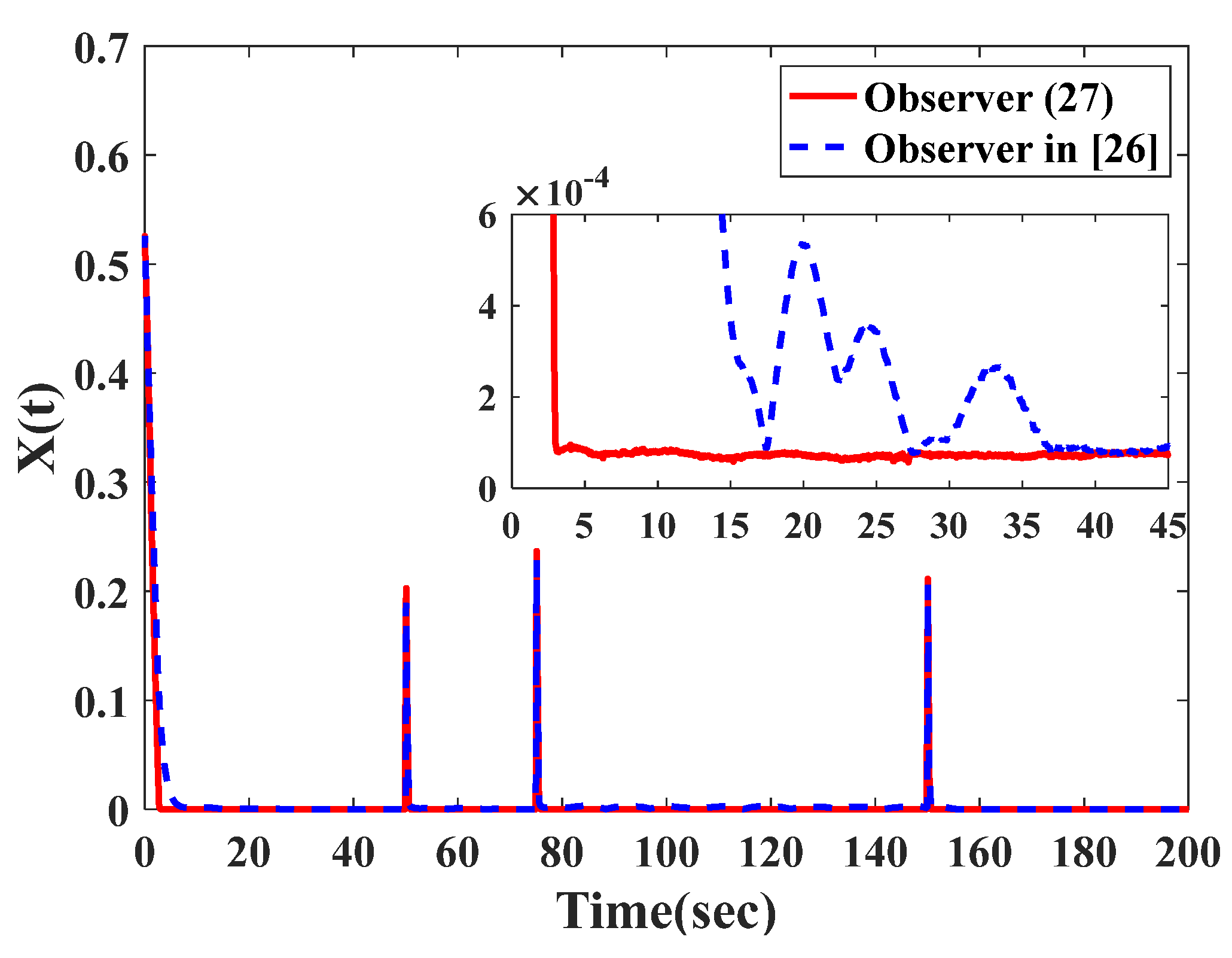
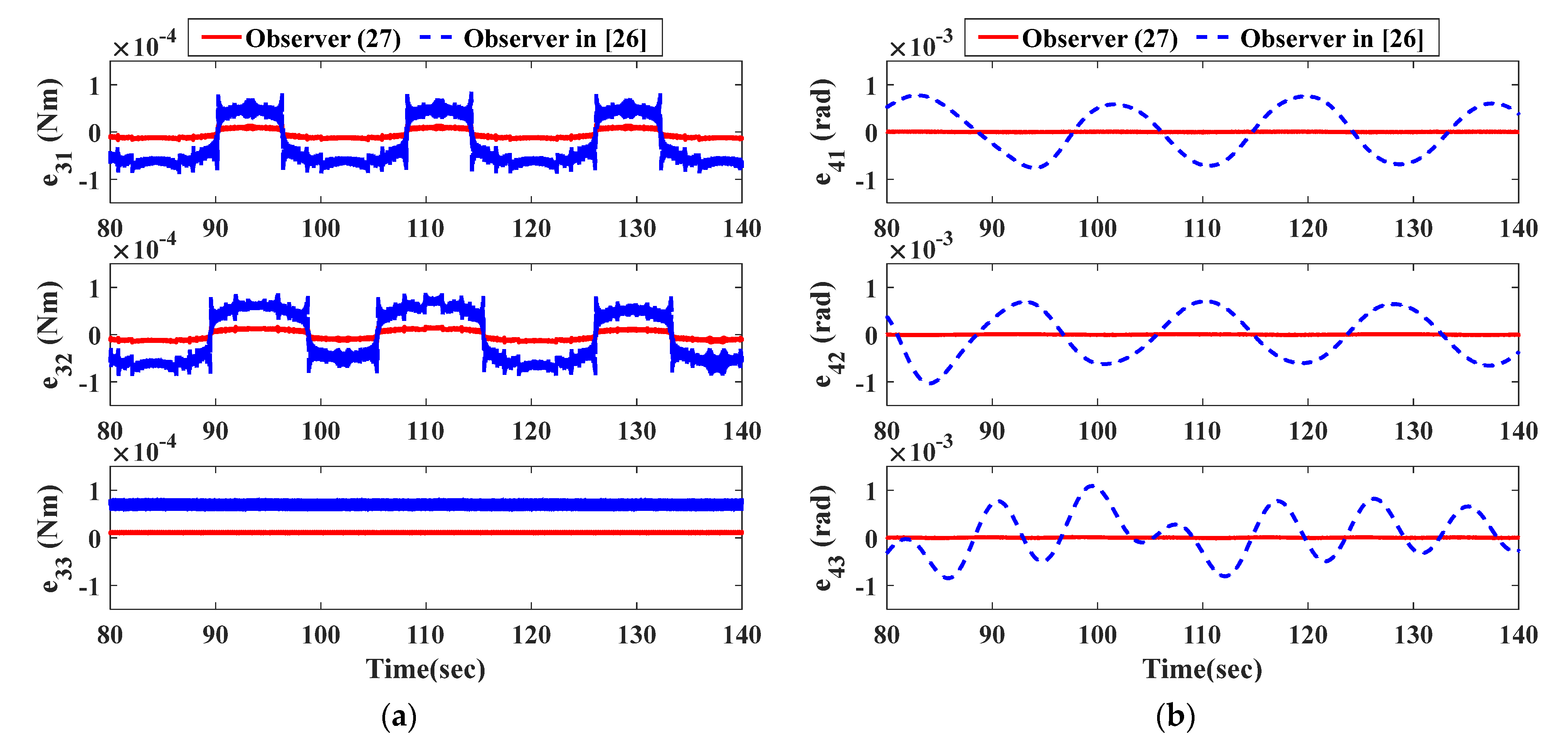
An improved sliding mode observer is proposed to estimate system states and faults simultaneously. Compared with the observer in [26], the steady-state performance is improved.

(b)

The multiplicative faults and additive faults of actuator and sensor are considered. The designed scheme is able to tolerate the lumped faults. The controller presented has a strong fault-tolerance ability such that the closed-loop attitude system is asymptotically stable.

(c)

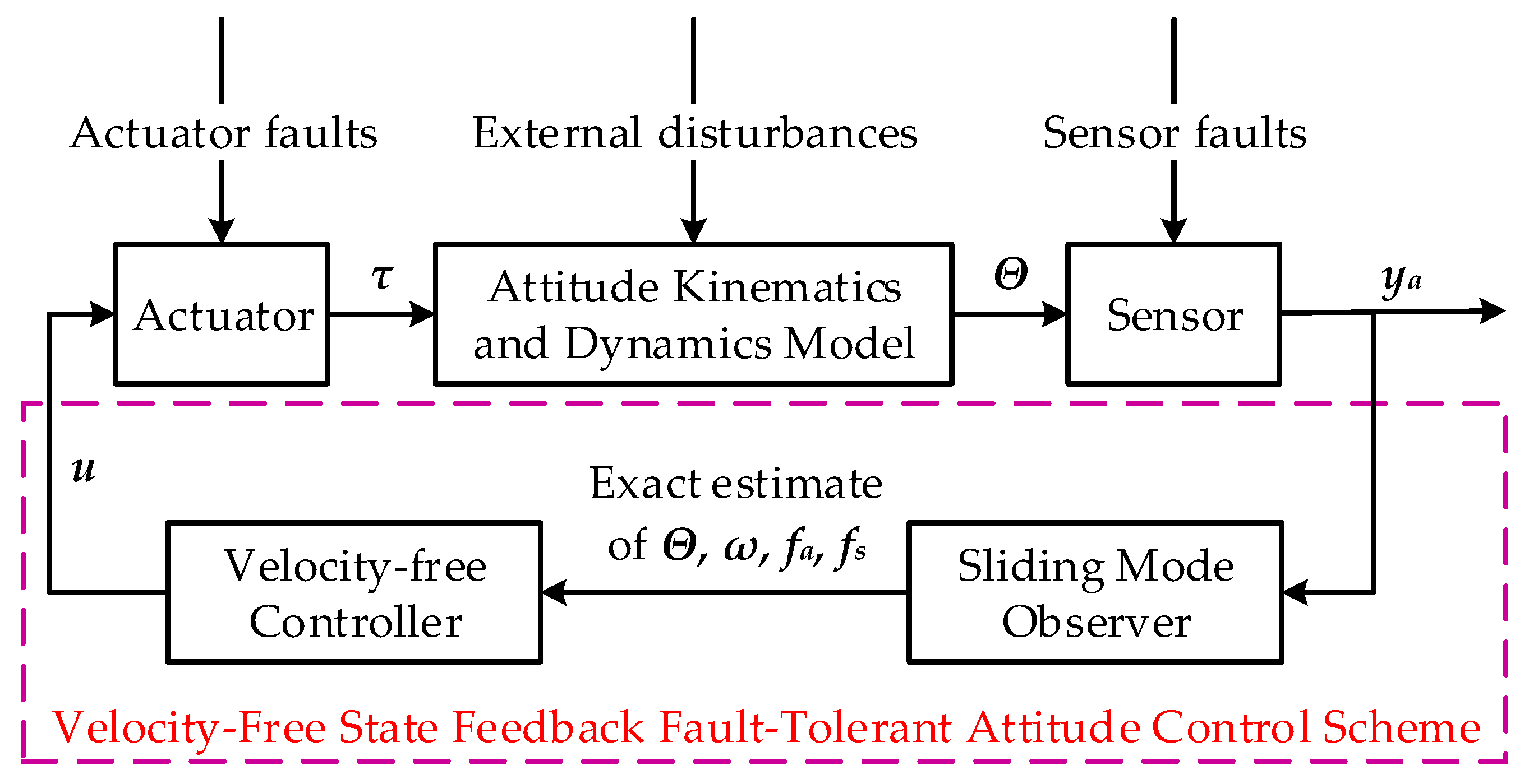
The proposed fault-tolerant control scheme does not require angular velocity measurements, which reduces satellite mass and the cost of airborne sensors.

The remainder of this paper is organized as follows. In Section 2, satellite attitude dynamics and actuator and sensor faults models are described. The required mathematical preliminaries are also given in this part. In Section 3, the proposed improved sliding mode observer and the state feedback fault-tolerant attitude controller are presented, respectively. Numerical simulation is provided to demonstrate the effectiveness of the proposed scheme in Section 4. Conclusions are given in Section 5.

2. Preliminaries

2.1. Notations and Lemmas

$I_n\in {\Re }^{n\times n}$ represents the identity matrix with a dimension $n$. $0_{n\times m}\in {\Re }^{n\times m}$ is an $n$ by $m$ zero matrix. $\left|\right|\hspace{0.17em}\cdot \hspace{0.17em}\left|\right|$ stands for the induced norm of a matrix or the Euclidean norm of a vector. ${\lambda }_{\min }(\cdot )$ and ${\lambda }_{\max }(\cdot )$ denote the minimum and maximum eigenvalues of a matrix, respectively. For a given scalar $\alpha >0$ and a vector $\mathit{x}={[\begin{array}{cccc}{x}_1& x_2& \dots & x_n\end{array}]}^T\in {\Re }^n$, the notation can be defined as follows: ${\mathrm{sig}}^{\alpha }(\mathit{x})={[\begin{array}{cccc}{\mathrm{sig}}^{\alpha }(x_1)& {\mathrm{sig}}^{\alpha }(x_2)& \cdots & {\mathrm{sig}}^{\alpha }(x_n)\end{array}]}^T$, where ${sig}^{\alpha }(x_i)=|x_i{|}^{\alpha }\mathrm{sgn}(x_i)$ and $\mathrm{sgn}(\cdot )$ denotes the sign function.

The function $\Gamma ({\displaystyle \mathit{x}},\alpha ,\beta )$ is defined as

$$\Gamma (\mathit{x},\alpha ,\beta )=\{\begin{array}{c}{\mathrm{sgn}}^{\alpha }(\mathit{x})\hspace{1em}\left|\right|\mathit{x}\left|\right|\le 1\\ {\mathrm{sgn}}^{\beta }(\mathit{x})\hspace{1em}\left|\right|\mathit{x}\left|\right|>1\end{array}$$

(1)

where $\mathit{x}\in {\Re }^n$, $0<\alpha <1$, and $\beta >1$.

For a given vector $\mathit{a}={[\begin{array}{ccc}{a}_1& a_2& a_3\end{array}]}^T\in {\Re }^3$, the notation ${\mathit{a}}^{\times }$ indicates the skew-symmetric matrix:

$${\mathit{a}}^{\times }=\left[\begin{array}{ccc}0& -a_3& a_2\\ a_3& 0& -a_1\\ -a_2& a_1& 0\end{array}\right]$$

(2)

Lemma 1 

[33].Consider the following nonlinear system of differential equations:

$$\dot{\mathit{x}}=\mathit{f}(t,\mathit{x}),\mathit{x}(0)=x_0$$

(3)

where$\mathit{x}\in {\Re }^n$is the system state and$\mathit{f}:{\Re }^{+}\times {\Re }^n\to {\Re }^n$is a continuous function defined in an open neighborhood$U$of the origin. If there is a positive definite function$V(\mathit{x}):{\Re }^n\to \Re$satisfying$\dot{V}(\mathit{x})\le -(\alpha V^p(\mathit{x})+\beta V^q(\mathit{x}))+\varsigma$, where$\alpha$, $\beta \in {\Re }^{+}$, $0<p<1$, $q>1$, and$0<\varsigma <\infty$, the trajectory of Equation (3) is practical fixed-time stable. The settling time$T$for the system to reach a steady state satisfies$T\le 1/\alpha (1-p)+1/\beta (q-1)$.

2.2. Satellite Attitude Dynamics Model

To describe the satellite attitude, three coordinate systems are commonly used: the inertial fixed reference coordinate frame ${ℱ}_I$, the orbital coordinate frame ${ℱ}_o$, and the body-fixed coordinate frame ${ℱ}_b$. The angular velocity ${\mathit{\omega }}_r$ of the body-fixed coordinate frame relative to the orbital coordinate frame is obtained by a yaw–pitch–roll sequence of rotations. It can be described by [35]

$${\mathit{\omega }}_r=\mathit{R}(\mathit{\Theta })\dot{\mathit{\Theta }}=\left[\begin{array}{ccc}1& 0& -\sin \theta \\ 0& \cos \varphi & \cos \theta \sin \varphi \\ 0& -\sin \varphi & \cos \theta \cos \varphi \end{array}\right]\left[\begin{array}{c}\dot{\varphi }\\ \dot{\theta }\\ \dot{\psi }\end{array}\right]$$

(4)

where $\mathit{\Theta }=\begin{array}{ccc}[\varphi & \theta & \psi \end{array}{]}^T\in {\Re }^3$ is the attitude Euler angle vector. The angular velocity $\mathit{\omega }={\left[\begin{array}{ccc}{\omega }_x& {\omega }_y& {\omega }_z\end{array}\right]}^T\in {\Re }^3$ of the body frame with respect to the inertial frame in the body frame is defined as

$$\mathit{\omega }={\mathit{\omega }}_r+{\mathit{\omega }}_O$$

(5)

where

$${\mathit{\omega }}_O=-\left[\begin{array}{c}\cos \theta \sin \psi \\ \cos \varphi \cos \psi +\sin \varphi \sin \theta \sin \psi \\ -\sin \varphi \cos \psi +\cos \varphi \sin \theta \sin \psi \end{array}\right]{\omega }_0$$

(6)

Here, ${\omega }_0$ is the orbital angular velocity. Substituting Equations (4) and (6) into Equation (5) and taking into account small Euler angle rotations, the attitude kinematics can be given by [21]

$$\mathit{\omega }={\left[\begin{array}{ccc}{\omega }_x& {\omega }_y& {\omega }_z\end{array}\right]}^T={\left[\begin{array}{ccc}\dot{\varphi }-{\omega }_0\psi & \dot{\theta }-{\omega }_0& \dot{\psi }+{\omega }_0\varphi \end{array}\right]}^T$$

(7)

The angular momentum is expressed as $\mathit{H}=I_b\mathit{\omega }$. In the case of considering the gravity gradient torque and the external disturbance torque, the attitude dynamics model of the rigid satellite can be described by [35]

$$I_b\dot{\mathit{\omega }}+{\mathit{\omega }}^{\times }{I}_b\mathit{\omega }=\mathit{\tau }+{\mathit{\tau }}_d+{\mathit{\tau }}_g$$

(8)

where $\mathit{\tau }=\begin{array}{ccc}[{\tau }_1& {\tau }_2& {\tau }_3\end{array}{]}^T\in {\Re }^3$ is the total torque generated by the actuator, ${\mathit{\tau }}_d=\begin{array}{ccc}[{\tau }_{d1}& {\tau }_{d2}& {\tau }_{d3}\end{array}{]}^T\in {\Re }^3$ is the external disturbance torque, and $I_b=\mathrm{diag}([\begin{array}{ccc}{I}_{b1}& I_{b2}& I_{b3}\end{array}])$ is the inertia matrix. In the case of a small attitude angle maneuver, the gravity gradient torque ${\mathit{\tau }}_g={[\begin{array}{ccc}{\tau }_{g1}& {\tau }_{g2}& {\tau }_{g3}\end{array}]}^T\in {\Re }^3$ can be approximated as

$${\mathit{\tau }}_g={\left[\begin{array}{ccc}-3{\omega }_0^2(I_{b2}-I_{b3})\varphi & -3{\omega }_0^2(I_{b1}-I_{b3})\theta & 0\end{array}\right]}^T$$

(9)

Substituting Equations (7) and (9) into Equation (8) yields

$$I_b\ddot{\mathit{\Theta }}+a_1\dot{\mathit{\Theta }}+a_0\mathit{\Theta }=\mathit{\tau }+{\mathit{\tau }}_d$$

(10)

Define a new state $\mathit{x}={[\begin{array}{cc}{\mathit{x}}_1^T& {\mathit{x}}_2^T\end{array}]}^T={[\begin{array}{cc}{\mathit{\Theta }}^T& {\dot{\mathit{\Theta }}}^T\end{array}]}^T$. Then, Equation (10) can be rewritten as:

$$\{\begin{array}{l}\dot{\mathit{x}}=A\mathit{x}+B\mathit{\tau }+D{\mathit{\tau }}_d\\ \mathit{y}=C\mathit{x}\end{array}$$

(11)

where $\mathit{x}\in {\Re }^6$, $\mathit{\tau }\in {\Re }^3$, ${\mathit{\tau }}_d\in {\Re }^3$, and $\mathit{y}\in {\Re }^6$ denote system state, total torque, external disturbance torque, and measurement output, respectively. The system parameter matrixes $A\in {\Re }^{6\times 6}$, $B\in {\Re }^{6\times 3}$, $D\in {\Re }^{6\times 3}$, and $C\in {\Re }^{6\times 6}$ are defined as

$$\begin{array}{c}{a}_0={\omega }_0^2\left[\begin{array}{ccc}4(I_{b2}-I_{b3})& 0& 0\\ 0& 3(I_{b1}-I_{b3})& 0\\ 0& 0& I_{b2}-I_{b1}\end{array}\right],a_1={\omega }_0\left[\begin{array}{ccc}\begin{array}{c}0\\ 0\\ I_{b1}-I_{b2}+I_{b3}\end{array}& \begin{array}{l}0\\ 0\\ 0\end{array}& \begin{array}{c}-I_{b1}+I_{b2}-I_{b3}\\ 0\\ 0\end{array}\end{array}\right],\\ A=\left[\begin{array}{cc}\begin{array}{c}{0}_3\\ -I_b^{-1}{a}_0\end{array}& \begin{array}{c}{I}_3\\ -I_b^{-1}{a}_1\end{array}\end{array}\right],B=D=\left[\begin{array}{l}{0}_3\\ I_b^{-1}\end{array}\right],c_1=\left[\begin{array}{ccc}0& 0& -{\omega }_0\\ 0& 0& 0\\ {\omega }_0& 0& 0\end{array}\right],C=\left[\begin{array}{cc}{I}_3& 0_3\\ c_1& I_3\end{array}\right].\end{array}$$

2.3. Faults Model

Referring to the definition of actuator faults in [36], the actuator faults can be divided into multiplicative faults and additive faults with the form

$$\mathit{\tau }=\rho \mathit{u}+{\mathit{u}}_f$$

(12)

where $\mathit{u}=\begin{array}{ccc}[u_1& u_2& u_3\end{array}{]}^T\in {\Re }^3$ represents the actuator commanded control torque; $\rho =\mathrm{diag}({[\begin{array}{ccc}{\rho }_1& {\rho }_2& {\rho }_3\end{array}]}^T)\in {\Re }^{3\times 3}$ denotes the degree of actuator failure, $0<{\rho }_i\le 1$, where $i=1,\hspace{0.17em}2,\hspace{0.17em}3$; and ${\mathit{u}}_f\in {\Re }^3$ stands for actuator additive faults. Equation (12) can be rewritten as

$$\mathit{\tau }=\mathit{u}+{\mathit{f}}_a$$

(13)

where the lumped actuator faults ${\mathit{f}}_a\in {\Re }^3$ can be defined as

$${\mathit{f}}_a=(\rho -I_3)\mathit{u}+{\mathit{u}}_f$$

(14)

In this paper, the fault-tolerant control of the satellite is studied under the condition of velocity-free measurements so that the actual measurement output only contains the attitude angle information. Considering partial failures and additive faults of the sensor, the expression of measurement output can be defined as

$${\mathit{y}}_a=\delta \mathit{y}+{\mathit{y}}_f$$

(15)

where ${\mathit{y}}_a\in {\Re }^3$ is the actual output of the sensor; ${\mathit{y}}_f\in {\Re }^3$ is sensor additive faults; and $\delta =\mathrm{diag}({[\begin{array}{ccc}{\delta }_1& {\delta }_2& {\delta }_3\end{array}]}^T)\in {\Re }^{3\times 3}$ denotes the degree of sensor failure, $0<{\delta }_i\le 1$, where $i=1,\hspace{0.17em}2,\hspace{0.17em}3$. Equation (14) can be rewritten as

$${\mathit{y}}_a=C\mathit{x}+{\mathit{f}}_s$$

(16)

where the lumped sensor faults ${\mathit{f}}_s\in {\Re }^3$ can be defined as

$${\mathit{f}}_s=(\delta -I_3)\mathit{y}+{\mathit{y}}_f$$

(17)

Combined with Equations (13) and (16), the system dynamics with actuator and sensor faults can be written as

$$\{\begin{array}{l}\dot{\mathit{x}}=A\mathit{x}+B(\mathit{u}+{\mathit{f}}_a)+D{\mathit{\tau }}_d\\ {\mathit{y}}_a=C\mathit{x}+{\mathit{f}}_s\end{array}$$

(18)

where ${\mathit{f}}_a\in {\Re }^3$ and ${\mathit{f}}_s\in {\Re }^3$ denote the lumped faults of the actuator and the lumped faults of the sensor, respectively. The parameter matrix $C=[\begin{array}{cc}{I}_3& 0_3\end{array}]\in {\Re }^{3\times 6}$. According to Equation (18), the following assumptions are made:

Assumption 1. 

There exist positive constants$k_{\Theta }$and$k_{\omega }$such that$\left|\right|\mathit{\Theta }\left|\right|\le k_{\Theta }$and$\left|\right|\mathit{\omega }\left|\right|\le k_{\omega }$for all$t\ge 0$.

Assumption 2. 

The external disturbances and actuator and sensor faults satisfy$\left|\right|{\mathit{\tau }}_d\left|\right|\le r_d$,$\left|\right|{\mathit{f}}_s\left|\right|\le r_s$,$\left|\right|{\mathit{f}}_a\left|\right|\le r_a$, and$\left|\right|{\dot{\mathit{f}}}_a\left|\right|\le r_{a1}$, where$r_d>0$, $r_s>0$,$r_a>0$, and$r_{a1}>0$are known constants. There is a known constant$\eta >0$such that$r_d+r_a+r_s+r_{a1}\le \eta$.

Remark 1. 

For the feedback control problem, the assumption of bounded system states and disturbances is necessary. Due to the physical limitation of the equipment, the attitude of the satellite and the output torque of the actuator are limited in practical engineering. If the external disturbance is infinite, the attitude system will not be controllable. Similar assumptions also can be found in related literature, such as Assumption 1 in [29] and Assumption 2 in [26].

2.4. Problem Statement

The objective of this work is stated as follows: for the satellite with simultaneous actuator faults, sensor faults, and velocity-free measurements, the designed observer is required to estimate the unknown system states and faults in real time. The velocity-free fault-tolerant controller is provided to asymptotically stabilize the attitude, i.e., $\mathit{\Theta }\to 0$ and $\mathit{\omega }\to 0$, even in the presence of external disturbances and actuator and sensor faults.

3. Observer-Based State Feedback Attitude Controller Design

In this section, a velocity-free state feedback fault-tolerant attitude controller (VSFTC) will be proposed to stabilize the attitude of the satellite. The structure of the closed-loop system is shown in Figure 1. This control structure includes two modules: an improved sliding mode observer is designed to estimate $\mathit{\Theta }$, $\mathit{\omega }$, ${\mathit{f}}_a$, and ${\mathit{f}}_s$ and a velocity-free controller is proposed by using the estimate information of the observer.

3.1. Improved Sliding Mode Observer Design

According to Equation (18), the augmented system is constructed as follows:

$$\{\begin{array}{l}\overline{E}\dot{\overline{\mathit{x}}}=\overline{A}\overline{\mathit{x}}+\overline{B}\mathit{u}+\overline{D}\overline{\mathit{d}}\\ {\mathit{y}}_a=\overline{C}\overline{\mathit{x}}\end{array}$$

(19)

where

$$\overline{\mathit{x}}=\left[\begin{array}{c}\mathit{x}\\ {\mathit{f}}_a\\ {\mathit{f}}_s\end{array}\right],\overline{\mathit{d}}=\left[\begin{array}{c}{\mathit{\tau }}_d\\ {\mathit{f}}_a+{\dot{\mathit{d}}}_a\\ {\mathit{f}}_s\end{array}\right],\overline{E}=\left[\begin{array}{ccc}{I}_6& 0_{6\times 3}& 0_{6\times 3}\\ 0_{3\times 6}& I_3& 0_3\\ 0_{3\times 6}& 0_3& 0_3\end{array}\right],$$

(20)

$$\overline{B}=\left[\begin{array}{l}B\\ 0_{6\times 3}\end{array}\right],\overline{C}=[\begin{array}{ccc}C& 0_3& I_3\end{array}],$$

(21)

$$\overline{A}=\left[\begin{array}{ccc}A& B& 0_{6\times 3}\\ 0_{3\times 6}& -I_3& 0_3\\ 0_{3\times 6}& 0_3& -I_3\end{array}\right],\overline{D}=\left[\begin{array}{ccc}D& 0_{6\times 3}& 0_{6\times 3}\\ 0_3& I_3& 0_3\\ 0_3& 0_3& I_3\end{array}\right]$$

(22)

Let $S=\overline{E}+\overline{F}\overline{C}\in {\Re }^{12\times 12}$; $\overline{F}\in {\Re }^{12\times 3}$ is selected as

$$\overline{F}={\left[\begin{array}{cccc}{0}_3^T& 0_3^T& 0_3^T& F^T\end{array}\right]}^T$$

(23)

where $F=\mathrm{diag}({[\begin{array}{ccc}{\sigma }_1& {\sigma }_2& {\sigma }_3\end{array}]}^T)\in {\Re }^{3\times 3}$ and ${\sigma }_i>0,i=1,2,3$, such that $S$ is non-singular.

Define $\overline{\overline{A}}=S^{-1}\overline{A}$, $\overline{\overline{B}}=S^{-1}\overline{B}$, $\overline{\overline{D}}=S^{-1}\overline{D}$, and $\overline{\overline{F}}=S^{-1}\overline{F}$. Then Equation (19) can be rewritten as

$$\{\begin{array}{l}\dot{\overline{\mathit{x}}}=\overline{\overline{A}}\overline{\mathit{x}}+\overline{\overline{B}}\mathit{u}+\overline{\overline{D}}\overline{\mathit{d}}+\overline{\overline{F}}{\dot{\mathit{y}}}_a\\ {\mathit{y}}_a=\overline{C}\overline{\mathit{x}}\end{array}$$

(24)

Let $\widehat{\overline{\mathit{x}}}$ and ${\widehat{\mathit{y}}}_a$ be estimates of $\overline{\mathit{x}}$ and ${\mathit{y}}_a$, respectively. The improved sliding mode observer is proposed as follows:

$$\dot{\widehat{\overline{\mathit{x}}}}=\overline{\overline{A}}\widehat{\overline{\mathit{x}}}+\overline{\overline{B}}\mathit{u}+\overline{\overline{D}}\mathit{\Delta }+\overline{\overline{F}}{\dot{\mathit{y}}}_a-L\Gamma (\overline{C}\mathit{e},\alpha ,\beta )-kL({\dot{\widehat{\mathit{y}}}}_a-{\dot{\mathit{y}}}_a)$$

(25)

where $\mathit{e}=\widehat{\overline{\mathit{x}}}-\overline{\mathit{x}}=[\begin{array}{cccc}{\mathit{e}}_1^T& {\mathit{e}}_2^T& {\mathit{e}}_3^T& {\mathit{e}}_4^T\end{array}{]}^T$ is the system state error vector; $0<\alpha <1$, $\beta >1$, $k>0$, and $L={[\begin{array}{cccc}{L}_1^T& L_2^T& L_3^T& L_4^T\end{array}]}^T\in {\Re }^{12\times 3}$ are the gain matrixes; $L_i=l_i{I}_3$; $l_i>0$, where $i=1,2,3,4$; and $\mathit{\Delta }$ is the compensation input. According to Assumption 2, $\mathit{\Delta }$ is designed as

$$\mathit{\Delta }=-(\eta +\epsilon )\mathrm{sgn}({\overline{\overline{D}}}^T{{\rm N}}^{-T}P\mathit{e})$$

(26)

where $\epsilon >0$ is a small scalar quantity and ${\rm N}$, $P\in {\Re }^{12\times 12}$ is the parameter matrix to be designed.

By defining $\mathit{z}=\widehat{\overline{\mathit{x}}}-\overline{\overline{F}}{\mathit{y}}_a+kL({\widehat{\mathit{y}}}_a-{\mathit{y}}_a)$, Equation (25) can be rewritten as

$$\{\begin{array}{l}\dot{\mathit{z}}=\overline{\overline{A}}\mathit{z}+\overline{\overline{B}}\mathit{u}+\overline{\overline{D}}\mathit{\Delta }+\overline{\overline{A}}(\overline{\overline{F}}+kL){\mathit{y}}_a-k\overline{\overline{A}}L{\widehat{\mathit{y}}}_a-L\Gamma (\overline{C}\mathit{e},\alpha ,\beta )\\ \widehat{\overline{\mathit{x}}}=\mathit{z}+(\overline{\overline{F}}+kL){\mathit{y}}_a-kL{\widehat{\mathit{y}}}_a\end{array}$$

(27)

where $\mathit{z}\in {\Re }^{12}$ is the system state and $\widehat{\overline{\mathit{x}}}$ is the system output.

According to Equations (24) and (25), the estimation errors can be given by

$$\dot{\mathit{e}}=\overline{\overline{A}}\mathit{e}+\overline{\overline{D}}\mathit{\Delta }-\overline{\overline{D}}\overline{\mathit{d}}-L\Gamma (\overline{C}\mathit{e},\alpha ,\beta )-kL\overline{C}\dot{\mathit{e}}$$

(28)

Define a matrix ${\rm N}=I_{12}+kL\overline{C}\in {\Re }^{12\times 12}$. According to the definition of $L$ and Equation (21), ${\rm N}$ is a non-singular matrix. Then, Equation (28) can be rewritten as

$$\dot{\mathit{e}}={{\rm N}}^{-1}(\overline{\overline{A}}\mathit{e}+\overline{\overline{D}}\mathit{\Delta }-\overline{\overline{D}}\overline{\mathit{d}}-L\Gamma (\overline{C}\mathit{e},\alpha ,\beta ))$$

(29)

Theorem 1. 

Consider the plant (18) subject to the actuator faults (14), sensor faults (17), and the external disturbances under Assumption 2. If the observer is designed according to Equation (27), there exist appropriate gain matrixes$L\in {\Re }^{12\times 3}$,$P\in {\Re }^{12\times 12}>0$, and$Q\in {\Re }^{12\times 12}>0$, satisfying:

$${(\overline{\overline{A}}-L\overline{C})}^T{{\rm N}}^{-T}P+P{{\rm N}}^{-1}(\overline{\overline{A}}-L\overline{C})+Q\le 0$$

(30)

such that the estimated states$\widehat{\overline{\mathit{x}}}$converges asymptotically to its actual states$\overline{\mathit{x}}$and the error dynamic system of Equation (29) is ultimately uniformly bounded.

Proof of Theorem 1. 

Define a Lyapunov function $V_1={\mathit{e}}^{T}P\mathit{e}$. The time derivative of $V_1$ along the trajectories of the error dynamics in Equation (29) leads to

$${\dot{V}}_1=2{\mathit{e}}^{T}P{{\rm N}}^{-1}\overline{\overline{A}}\mathit{e}+2{\mathit{e}}^{T}P{{\rm N}}^{-1}\overline{\overline{D}}\mathit{\Delta }-2{\mathit{e}}^{T}P{{\rm N}}^{-1}\overline{\overline{D}}\overline{\mathit{d}}-2{\mathit{e}}^{T}P{{\rm N}}^{-1}L\Gamma (\overline{C}\mathit{e},\alpha ,\beta )$$

(31)

According to Equation (1), $\Gamma (x,\alpha ,\beta )$ is a piecewise function. We discuss ${\dot{V}}_1$ in two parts: Part 1 ($\left|\right|\overline{C}\mathit{e}\left|\right|\le 1$) and Part 2 ($\left|\right|\overline{C}\mathit{e}\left|\right|>1$).

Part 1: $\left|\right|\overline{C}\mathit{e}\left|\right|\le 1$. Based on Equation (1), Equation (31) can be rewritten as

$${\dot{V}}_1=2{\mathit{e}}^{T}P{{\rm N}}^{-1}\overline{\overline{A}}\mathit{e}+2{\mathit{e}}^{T}P{{\rm N}}^{-1}\overline{\overline{D}}\mathit{\Delta }-2{\mathit{e}}^{T}P{{\rm N}}^{-1}\overline{\overline{D}}\overline{\mathit{d}}\hspace{0.17em}-2{\mathit{e}}^{T}P{{\rm N}}^{-1}L{\mathrm{sig}}^{\alpha }(\overline{C}\mathit{e})$$

(32)

Since $\left|\right|\overline{C}\mathit{e}\left|\right|\le 1$ and $0<\alpha <1$, we have $\left|\right|\overline{C}\mathit{e}|{|}^{\alpha }\ge \left|\right|\overline{C}\mathit{e}\left|\right|$. Substituting it into Equation (32) yields

$${\dot{V}}_1\le 2{\mathit{e}}^{T}P{{\rm N}}^{-1}\overline{\overline{A}}\mathit{e}-2{\mathit{e}}^{T}P{{\rm N}}^{-1}L\overline{C}\mathit{e}+2{\mathit{e}}^{T}P{{\rm N}}^{-1}\overline{\overline{D}}\mathit{\Delta }-2{\mathit{e}}^{T}P{{\rm N}}^{-1}\overline{\overline{D}}\overline{\mathit{d}}$$

(33)

According to Assumption 2, $\left|\right|\overline{\mathit{d}}\left|\right|\le \eta$. If the inequality in Equation (30) holds, substituting Equation (26) into Equation (33), we have

$$\begin{array}{l}{\dot{V}}_1\le 2{\mathit{e}}^{T}P{{\rm N}}^{-1}\overline{\overline{A}}\mathit{e}-2{\mathit{e}}^{T}P{{\rm N}}^{-1}L\overline{C}\mathit{e}+2e^{T}P{{\rm N}}^{-1}\overline{\overline{D}}\mathit{\Delta }\hspace{0.17em}+2\eta \left|\right|{\mathit{e}}^{T}P{{\rm N}}^{-T}\overline{\overline{D}}\left|\right|\\ \le {\mathit{e}}^T({(\overline{\overline{A}}-L\overline{C})}^T{{\rm N}}^{-T}P+P{{\rm N}}^{-1}(\overline{\overline{A}}-L\overline{C}))\mathit{e}\hspace{0.17em}+2\left|\right|{\mathit{e}}^{T}P{{\rm N}}^{-T}\overline{\overline{D}}\left|\right|(-(\epsilon +\eta )+\eta )\\ \le -{\mathit{e}}^{T}Q\mathit{e}-2\epsilon \left|\right|{\mathit{e}}^{T}P{{\rm N}}^{-T}\overline{\overline{D}}\left|\right|\end{array}$$

(34)

From the standard inequality for quadratic forms, we obtain ${\lambda }_{\min }(Q)\left|\right|\mathit{e}|{|}^2\le V_1\le {\lambda }_{\max }(Q)\left|\right|\mathit{e}|{|}^2$. For $\epsilon >0$, the inequality in Equation (34) can also be rewritten as

$${\dot{V}}_1\le -{\lambda }_{\min }(Q)\left|\right|\mathit{e}|{|}^2\le 0$$

(35)

Part 2: $\left|\right|\overline{C}\mathit{e}\left|\right|>1$. Based on Equation (1), Equation (31) can be rewritten as

$${\dot{V}}_1=2{\mathit{e}}^{T}P{{\rm N}}^{-1}\overline{\overline{A}}\mathit{e}+2{\mathit{e}}^{T}P{{\rm N}}^{-1}\overline{\overline{D}}\mathit{\Delta }-2{\mathit{e}}^{T}P{{\rm N}}^{-1}\overline{\overline{D}}\overline{\mathit{d}}-2{\mathit{e}}^{T}P{{\rm N}}^{-1}L{\mathrm{sig}}^{\beta }(\overline{C}\mathit{e})$$

(36)

Since $\left|\right|\overline{C}\mathit{e}\left|\right|>1$ and $\beta >1$, we have $\left|\right|\overline{C}\mathit{e}|{|}^{\beta }\ge \left|\right|\overline{C}\mathit{e}\left|\right|$. Substituting it into Equation (36) yields

$${\dot{V}}_1\le 2{\mathit{e}}^{T}P{{\rm N}}^{-1}\overline{\overline{A}}\mathit{e}-2{\mathit{e}}^{T}P{{\rm N}}^{-1}L\overline{C}\mathit{e}+2{\mathit{e}}^{T}P{{\rm N}}^{-1}\overline{\overline{D}}\mathit{\Delta }-2{\mathit{e}}^{T}P{{\rm N}}^{-1}\overline{\overline{D}}\overline{\mathit{d}}$$

(37)

Following the same procedure in Part 1, ${\dot{V}}_1$ satisfies

$${\dot{V}}_1\le -{\lambda }_{\min }(Q)\left|\right|\mathit{e}|{|}^2\le 0$$

(38)

With the combination of Part 1 and Part 2, we have ${\dot{V}}_1\le 0$ when Equation (30) holds. According to the Lyapunov stability theorem, the errors system in Equation (29) is asymptotically stable. This completes the proof of Theorem 1. □

3.2. Velocity-Free State Feedback Fault-Tolerant Attitude Controller Design

The parameter matrix of the observer in Equation (25) is expressed as follows:

$$\overline{\overline{A}}=\left[\begin{array}{cccc}{\overline{\overline{A}}}_{11}& {\overline{\overline{A}}}_{12}& {\overline{\overline{A}}}_{13}& {\overline{\overline{A}}}_{14}\\ {\overline{\overline{A}}}_{21}& {\overline{\overline{A}}}_{22}& {\overline{\overline{A}}}_{23}& {\overline{\overline{A}}}_{24}\\ {\overline{\overline{A}}}_{31}& {\overline{\overline{A}}}_{32}& {\overline{\overline{A}}}_{33}& {\overline{\overline{A}}}_{34}\\ {\overline{\overline{A}}}_{41}& {\overline{\overline{A}}}_{42}& {\overline{\overline{A}}}_{43}& {\overline{\overline{A}}}_{44}\end{array}\right],\overline{\overline{B}}=\left[\begin{array}{c}{\overline{\overline{B}}}_1\\ {\overline{\overline{B}}}_2\\ {\overline{\overline{B}}}_3\\ {\overline{\overline{B}}}_4\end{array}\right],\overline{\overline{D}}=\left[\begin{array}{c}{\overline{\overline{D}}}_1\\ {\overline{\overline{D}}}_2\\ {\overline{\overline{D}}}_3\\ {\overline{\overline{D}}}_4\end{array}\right]$$

where ${\overline{\overline{A}}}_{i,j}\in R^{3\times 3}$, ${\overline{\overline{B}}}_i\in R^{3\times 3}$, and ${\overline{\overline{D}}}_i\in R^{3\times 3}$, where $i,j=1,2,3,4$. According to the parameter setting in Equations (11) and (19), ${\overline{\overline{A}}}_{1,2}=I_3$ and ${\overline{\overline{A}}}_{2,3}={\overline{\overline{B}}}_2=I_b^{-1}$. By decomposing Equation (25), the differential forms of attitude angle estimation ${\widehat{\mathit{x}}}_1$ and attitude angle velocity estimation ${\widehat{\mathit{x}}}_2$ can respectively be described as

$${\dot{\widehat{\mathit{x}}}}_1={\widehat{\mathit{x}}}_2-L_1\Gamma (\overline{C}\mathit{e},\alpha ,\beta )-k{L}_1\overline{C}\dot{\mathit{e}}$$

(39)

$${\dot{\widehat{\mathit{x}}}}_2={\overline{\overline{A}}}_{2,1}{\widehat{\mathit{x}}}_1+{\overline{\overline{A}}}_{2,2}{\widehat{\mathit{x}}}_2+I_b^{-1}{\widehat{\mathit{f}}}_a+I_b^{-1}\mathit{u}+{\overline{\overline{D}}}_2\mathit{\Delta }-k{L}_2\overline{C}\dot{\mathit{e}}-L_2\Gamma (\overline{C}\mathit{e},\alpha ,\beta )$$

(40)

Based on Theorem 1, the following assumption is proposed:

Assumption 3. 

The feedback term$\Gamma (\overline{C}\mathit{e},\alpha ,\beta )+k({\dot{\widehat{\mathit{y}}}}_a-{\dot{\mathit{y}}}_a)$of Equation (25) can rewritten as$\Gamma (\overline{C}\mathit{e},\alpha ,\beta )+k\overline{C}\dot{\mathit{e}}$. There exists a positive scalar$k_e$, satisfying$\left|\right|\Gamma (\overline{C}\mathit{e},\alpha ,\beta )+k\overline{C} \dot{\mathit{e}} \left|\right|\le k_e$, for all$t\ge 0$.

Remark 2. 

It has been proved in Theorem 1 that the observer errors system is asymptotically stable, which means that both$\mathit{e}$and$\dot{\mathit{e}}$can converge to neighbors of zero. Therefore, the observer feedback term$\Gamma (\overline{C}\mathit{e},\alpha ,\beta )+k\overline{C}\dot{\mathit{e}}$is bounded. Assumption 3 is reasonable.

Theorem 2. 

Consider the satellite attitude model (18) with the actuator, sensor faults, and velocity-free measurements. Based on the observer in Equation (27), the controller is designed as

$$\begin{array}{l}\mathit{u}=I_b(-{\overline{\overline{A}}}_{2,1}{\widehat{\mathit{x}}}_1-{\overline{\overline{A}}}_{2,2}{\widehat{\mathit{x}}}_2-{\overline{\overline{D}}}_2\mathit{\Delta }+L_2\Gamma (\overline{C}\mathit{e},\alpha ,\beta )+k{L}_2\overline{C}\dot{\mathit{e}}\\ \hspace{0.17em}\hspace{0.17em}\hspace{0.17em}\hspace{0.17em}\hspace{0.17em}\hspace{0.17em}\hspace{0.17em}+g_1( p{k}_2{\xi }_1+q{k}_3{\xi }_2)(-{\widehat{\mathit{x}}}_2+L_1\Gamma (\overline{C}\mathit{e},\alpha ,\beta )+k{L}_1\overline{C}\dot{\mathit{e}})\\ \hspace{0.17em}\hspace{0.17em}\hspace{0.17em}\hspace{0.17em}\hspace{0.17em}\hspace{0.17em}\hspace{0.17em}-g_1({\gamma }_1{\mathrm{sig}}^p(\mathit{s})+{\gamma }_2{\mathrm{sig}}^q(\mathit{s})+{\gamma }_3\mathit{s}+g_1{\widehat{\mathit{x}}}_1))-{\widehat{\mathit{f}}}_a\end{array}$$

(41)

where${\xi }_1=\mathrm{diag}(|{\widehat{\mathit{x}}}_1{|}^{p-1})$,${\xi }_2=\mathrm{diag}(|{\widehat{\mathit{x}}}_1{|}^{q-1})$,$k_i$,${\gamma }_i>0$ $(i=1,2,3)$,$p\in (0,1)$,$q>1$, and$g_1=1/k_1$;$\mathit{s}$is defined as follows:

$$\mathit{s}=k_1{\widehat{\mathit{x}}}_2+k_2{\mathrm{sig}}^p({\widehat{\mathit{x}}}_1)+k_3{\mathrm{sig}}^q({\widehat{\mathit{x}}}_1)$$

(42)

Then, the estimated attitude angle and the estimated attitude angular velocity converge to a steady state within a fixed time. According to Theorem 1, the observer dynamic error is asymptotically stable. Therefore, the satellite attitude system asymptotically stabilizes.

Proof of Theorem 2. 

Using Equations (39) and (40), the time derivative of $\mathit{s}$ becomes

$$\begin{array}{l}\dot{\mathit{s}}=k_1{\dot{\widehat{\mathit{x}}}}_2+p{k}_2{\xi }_1{\dot{\widehat{\mathit{x}}}}_1+q{k}_3{\xi }_2{\dot{\widehat{\mathit{x}}}}_1\\ \hspace{0.17em}\hspace{0.17em}\hspace{0.17em}=k_1({\overline{\overline{A}}}_{2,1}{\widehat{\mathit{x}}}_1+{\overline{\overline{A}}}_{2,2}{\widehat{\mathit{x}}}_2+I_b^{-1}{\widehat{\mathit{f}}}_a+I_b^{-1}\mathit{u}+{\overline{\overline{D}}}_2\mathit{\Delta }-L_2\Gamma (\overline{C}\mathit{e},\alpha ,\beta )-k{L}_2\overline{C}\dot{\mathit{e}})\\ \hspace{0.17em}\hspace{0.17em}\hspace{0.17em}\hspace{0.17em}\hspace{0.17em}\hspace{0.17em}\hspace{0.17em}+(p{k}_2{\xi }_1+q{k}_3{\xi }_2)({\widehat{\mathit{x}}}_2-L_1\Gamma (\overline{C}\mathit{e},\alpha ,\beta )-k{L}_1\overline{C}\dot{\mathit{e}})\end{array}$$

(43)

Substituting Equation (41) into Equation (43) yields

$$\dot{\mathit{s}}=-{\gamma }_1{\mathrm{sig}}^p(\mathit{s})-{\gamma }_2{\mathrm{sig}}^q(\mathit{s})-{\gamma }_3\mathit{s}-g_1{\widehat{\mathit{x}}}_1$$

(44)

Then, define a new state vector $\mathit{\zeta }={[\begin{array}{cc}{\mathit{s}}^T& {\widehat{\mathit{x}}}^T{}_1\end{array}]}^T$. Choose a candidate Lyapunov function as $V_2={\mathit{\zeta }}^T\mathit{\zeta }$. Computing its time derivative by using Equations (39) and (44) gives

$$\begin{array}{c}{\dot{V}}_2=2{\dot{\mathit{\zeta }}}^T\mathit{\zeta }=2{\mathit{s}}^T \mathit{s} \dot{}+2{\widehat{\mathit{x}}}^T{}_1\dot{\widehat{\mathit{x}}}\hfill \\ \hspace{0.17em}=2{\mathit{s}}^T(-{\gamma }_1{\mathrm{sig}}^p(\mathit{s})-{\gamma }_2{\mathrm{sig}}^q(\mathit{s})-{\gamma }_3\mathit{s}-g_1{\widehat{\mathit{x}}}_1)\hspace{0.17em}+2{\widehat{\mathit{x}}}^T{}_1({\widehat{\mathit{x}}}_2-L_1\Gamma (\overline{C}\mathit{e},\alpha ,\beta )-k{L}_1\overline{C}\dot{\mathit{e}})\end{array}$$

(45)

The expression ${\widehat{\mathit{x}}}_2=g_1(\mathit{s}-k_2{\mathrm{sig}}^p({\widehat{\mathit{x}}}_1)-k_3{\mathrm{sig}}^q({\widehat{\mathit{x}}}_1))$ can be obtained by Equation (42). Substituting it into Equation (45) yields

$$\begin{array}{l}{\dot{V}}_2=-2({\gamma }_1{\mathit{s}}^T{\mathrm{sig}}^p(\mathit{s})+{\gamma }_2{\mathit{s}}^T{\mathrm{sig}}^q(\mathit{s})+{\gamma }_3{\mathit{s}}^T\mathit{s}+g_1{\mathit{s}}^T{\widehat{\mathit{x}}}_1-g_1{\widehat{\mathit{x}}}^T{}_1\mathit{s}+g_1{k}_2{\widehat{\mathit{x}}}^T{}_1{\mathrm{sig}}^p({\widehat{\mathit{x}}}_1)\\ \hspace{0.17em}\hspace{0.17em}+g_1{k}_3{\widehat{\mathit{x}}}^T{}_1{\mathrm{sig}}^q({ \mathit{x} ^}_1)+{\widehat{\mathit{x}}}^T{}_1{L}_1(\Gamma (\overline{C}\mathit{e},\alpha ,\beta )+k\overline{C}\dot{\mathit{e}}))\\ \le -2{\chi }_1{\mathit{\zeta }}^T{\mathrm{sig}}^p(\mathit{\zeta })-2{\chi }_2{\mathit{\zeta }}^T{\mathrm{sig}}^q(\mathit{\zeta })-2{\widehat{\mathit{x}}}^T{}_1{L}_1(\Gamma (\overline{C}\mathit{e},\alpha ,\beta )+k\overline{C}\dot{\mathit{e}})\\ \le -2{\chi }_1{V}_2{}^{{\alpha }_1}-2{\chi }_2{V}_2{}^{{\beta }_1}-2{\widehat{\mathit{x}}}^T{}_1{L}_1(\Gamma (\overline{C}\mathit{e},\alpha ,\beta )+k\overline{C}\dot{\mathit{e}})\end{array}$$

(46)

where ${\alpha }_1=(1+p)/2$, ${\beta }_1=(1+q)/2$, ${\chi }_1=\min \{{\gamma }_1,g_1{k}_2\}$, and ${\chi }_2=\min \{{\gamma }_2,g_1{k}_3\}$. According to Assumption 1 and Theorem 1, there exists $k_4>0$ such that $\left|\right|{\widehat{\mathit{x}}}_1\left|\right|\le k_4$. By Assumption 3, the upper bound of the term ${\widehat{\mathit{x}}}_1^T{L}_1(\Gamma (\overline{C}\mathit{e},\alpha ,\beta )+k\overline{C}\dot{\mathit{e}})$ is obtained:

$${\widehat{\mathit{x}}}^T{}_1{L}_1(\Gamma (\overline{C}\mathit{e},\alpha ,\beta )+k\overline{C}\dot{\mathit{e}})\le l_1\left|\right|{\widehat{\mathit{x}}}_1^T\left|\right|\hspace{0.17em}\left|\right|\Gamma (\overline{C}\mathit{e},\alpha ,\beta )+k\overline{C} \dot{\mathit{e}} \left|\right|\le l_1{k}_4{k}_e<\infty$$

(47)

Substituting Equation (47) into Equation (46) yields

$${\dot{V}}_2\le -2{\chi }_1{V}_2{}^{{\alpha }_1}-2{\chi }_2{V}_2{}^{{\beta }_1}+\upsilon$$

(48)

where $\upsilon =2l_1{k}_4{k}_e$. From the definitions of $p$ and $q$, ${\alpha }_1$ and ${\beta }_1$ satisfy $0<{\alpha }_1<1$ and ${\beta }_1>1$, respectively. According to Lemma 1, if the controller is chosen as Equation (41), $\mathit{s}$ and ${\widehat{\mathit{x}}}_1$ will converge in the neighborhood of zero within a fixed time. The systems in Equations (39) and (40) are practical fixed-time stable. Moreover, the setting time $T$ is given by

$$T\le T_{\max }=\frac{1}{2{\chi }_1(1-{\alpha }_1)}+\frac{1}{2{\chi }_2({\beta }_1-1)}$$

(49)

Theorem 1 proves that the observer errors are asymptotically stable, which means that the satellite attitude is asymptotically stable. Thus, the argument stated in Theorem 2 holds and the proof is completed. □

4. Simulation Results

In this section, simulation results are presented to verify the effectiveness of the proposed observer (Equation (27)) and VSFTC (Equation (41)). Consider a small angular maneuvering satellite with actuator and sensor faults without velocity information. The inertia matrix is

$$I_b=\mathrm{diag}({[\begin{array}{ccc}18.73& 20.77& 23.63\end{array}]}^T)\mathrm{kg}\cdot {\mathrm{m}}^2$$

(50)

The initial attitude angle is chosen as

$$\mathit{\Theta }(0)={\mathit{x}}_1(0)={[\begin{array}{ccc}0.0859& -0.1628& 0.1109\end{array}]}^T\mathrm{rad}$$

(51)

The initial velocity is chosen as

$$\mathit{\omega }(0)={\mathit{x}}_2(0)={[\begin{array}{ccc}-0.0415& 0.0496& -0.0557\end{array}]}^T\mathrm{rad}/\mathrm{s}$$

(52)

The satellite orbital angular velocity is ${\omega }_0=0.0012\mathrm{rad}/\mathrm{s}$. The external disturbance torque is set as follows:

$${\mathit{\tau }}_d=1.5\times {10}^{-5}\times \left[\begin{array}{c}3\cos ({\omega }_{0}t)+1\\ 1.5\sin ({\omega }_{0}t)+3\cos ({\omega }_{0}t)\\ 3\sin ({\omega }_{0}t)+1\end{array}\right]\mathrm{Nm}$$

(53)

The initial values of observer system states are $\widehat{\overline{\mathit{x}}}(0)={[\begin{array}{cc}{0}^T& {\mathit{y}}_a^T\end{array}]}^T$.

Non-gyroscopic attitude sensors are equipped to measure the attitude angle $\mathit{\Theta }$. A zero-mean Gaussian random noise with the variance of $1\times {10}^{-5}$ is added to the attitude sensors model. The parameters of Equation (27) are chosen as $\eta =0.5$, $\epsilon =0.0001$, ${\sigma }_1={\sigma }_2={\sigma }_3=40$, $l_1=7.68$, $l_2=0.66$, $l_3=0.09$, $l_4=6.44$, $k=0.001$, $\alpha =0.6$, and $\beta =1.4$. The gains for the observer scheme in [26] are set as $\eta =0.5$, $\epsilon =0.0001$, ${\sigma }_1={\sigma }_2={\sigma }_3=40$, and $L={\left[\begin{array}{cccc}7.68I_3& 0.66I_3& 0.09I_3& 6.44I_3\end{array}\right]}^T$. The gains for the controller in Equation (41) are set as ${\gamma }_1=1.4$, ${\gamma }_2=0.84$, ${\gamma }_3=0.7$, $k_1=1$, $k_2=k_3=1.1$, $p=0.9$, and $q=1.4$.

4.1. Observer-Based PD Controller Simulation

In this part of the simulation, the performance of the proposed observer (Equation (27)) is compared with the observer method in [26]. The observer parameters in [26] are consistent with the above sets in this paper. To better display the effectiveness of the proposed observer, a PD controller is set as

$$\mathit{u}=-3I_3{\widehat{\mathit{x}}}_1-5I_3{\widehat{\mathit{x}}}_2$$

(54)

For a satellite without angular velocity measurements, the lumped faults, including multiplicative faults and additive faults, are designed as

$${\mathit{f}}_a=\{\begin{array}{c}{f}_{a_1}=\{\begin{array}{l}-0.15\\ 0.2\sin (0.35t)-0.1\end{array}\hspace{1em}\hspace{1em}\hspace{1em}\hspace{1em}\\ f_{a_2}=\{\begin{array}{l}0.2\\ 0.2\sin (0.35t)-0.1\cos (0.15t)\end{array}\\ f_{a_3}=\{\begin{array}{l}0.1\sin (0.25t)\\ 0.15\end{array}\hspace{1em}\hspace{1em}\hspace{1em}\hspace{1em}\hspace{1em}\hspace{1em}\end{array}\begin{array}{l}\hspace{0.17em}\hspace{0.17em}50\le t<75\hspace{0.17em}\hspace{0.17em}\hfill \\ \hspace{0.17em}\hspace{0.17em}75\le t<150\hfill \\ \hspace{0.17em}\hspace{0.17em}50\le t<75\hspace{0.17em}\hspace{0.17em}\hfill \\ \hspace{0.17em}\hspace{0.17em}75\le t<150\hfill \\ \hspace{0.17em}\hspace{0.17em}\hspace{0.17em}\hspace{0.17em}0\le t<100\hfill \\ 100\le t<150\hfill \end{array}\hspace{0.17em}\hspace{1em}(\rho -I_3)\mathit{u}=\{\begin{array}{l}-0.15u_1\\ -0.2u_2\\ -0.3u_3\end{array}\hspace{1em}\begin{array}{c}0\le t<75\\ 0\le t<75\\ 0\le t<75\end{array}$$

(55)

$${\mathit{f}}_s=\{\begin{array}{l}0.02\sin (0.025\pi t)+0.1\hfill \\ 0.03\sin (0.02\pi t)+0.05\hfill \\ 0.025\cos (0.015\pi t)+0.06\hfill \end{array}\hspace{1em}\begin{array}{c}0\le t\le 200\\ 0\le t\le 200\\ 0\le t\le 200\end{array}\hspace{0.17em}\hspace{1em}\hspace{0.17em}(\delta -I_3){\mathit{y}}_a=\{\begin{array}{l}-0.25y_{a1}\\ -0.4y_{a2}\\ -0.3y_{a3}\end{array}\hspace{1em}\begin{array}{c}0\le t\le 200\\ 0\le t\le 200\\ 0\le t\le 200\end{array}$$

(56)

where $u_i$ and $y_{ai}$ represent the triaxial component of $\mathit{u}$ and ${\mathit{y}}_a$, respectively, and $t$ is in seconds.

The curves in Figure 2 and Figure 3 illustrate the time response of attitude estimation errors ${\mathit{e}}_1$ and angular velocity estimation errors ${\mathit{e}}_2$ by two observers. It can be clearly seen from Figure 2 and Figure 3 that the observation errors of $\mathit{\Theta }$ and $\mathit{\omega }$ under the observer in Equation (27) can respectively converge to $\left|e_{1i}\right|\le 2\times {10}^{-5}$ and $\left|e_{2i}\right|\le 2\times {10}^{-6}$ within 2.8 s; the observation errors of $\mathit{\Theta }$ and $\mathit{\omega }$ under the observer in [26] can respectively converge to $\left|e_{1i}\right|\le 3\times {10}^{-4}$ and $\left|e_{2i}\right|\le 2\times {10}^{-5}$ within 16 s.

Figure 4 and Figure 5, respectively, show the reconstruction errors of the observer in Equation (27) and the observer in [26] for actuator faults ${\mathit{f}}_a$ and sensor faults ${\mathit{f}}_s$. It can be seen in Figure 4a and Figure 5a that the reconstruction using the proposed observer is achieved accurately within 2.8 s with steady-state accuracies of $\left|e_{3i}\right|,\left|e_{4i}\right|\le 2\times {10}^{-5}$. In Figure 4b, the observer in [26] also shows good reconstruction performance, and the actuator faults converge to $\left|e_{3i}\right|\le 1\times {10}^{-4}$ at 2.8 s. Figure 5b shows that the reconstruction of sensor faults under the observer in [26] can converge to $\left|e_{4i}\right|\le 3\times {10}^{-4}$ within 16 s. The summary can also be found in

Table 1. The comparison results of the observer in Equation (27) and the observer in [26].

	Observer (Equation (27))		Observer in [26]
	Ultimate Bound	Settling Time	Ultimate Bound	Settling Time
${\mathit{e}}_1$ (rad)	$2\times {10}^{-5}$	2.8	$3\times {10}^{-4}$	16
${\mathit{e}}_2$ (rad/s)	$2\times {10}^{-6}$	2.8	$2\times {10}^{-5}$	16
${\mathit{e}}_3$ (Nm)	$2\times {10}^{-5}$	2.8	$1\times {10}^{-4}$	2.8
${\mathit{e}}_4$ (rad)	$2\times {10}^{-5}$	2.8	$3\times {10}^{-4}$	16

.

To give a more instructive comparison of the two observers, the function ${\rm X}(t)=\left|\right|\mathit{e}(t)\left|\right|$ is defined motivated by [29] and its time response is shown in Figure 6. From Figure 6, it is obvious that the proposed observer (Equation (27)) provides a faster convergence rate than the observer in [26]. In Figure 7 and Figure 8, the steady-state error performances of the two observers are shown during the same fault period. The observer proposed has a higher steady-state accuracy than the observation scheme in [26].

4.2. VSFTC Simulation

To verify the applicability of the observation method, the actuator faults are redefined in this section. The sensor faults follow Equation (57). Due to the accurate reconstruction of the actuator and sensor faults supplied by Equation (27), the controller in Equation (41) can completely compensate for the effects of actuator and sensor faults. The accurate attitude information can be obtained. Thus, the controller can guarantee the asymptotic stability of satellite attitude and angular velocity. The actuator faults are selected as follows:

$${\mathit{f}}_a=\{\begin{array}{c}{f}_{a_1}=\{\begin{array}{l}-0.15\\ 0.1\sin (0.2t+\pi /3)-0.1\end{array}\hspace{0.17em}\hspace{0.17em}\hspace{1em}\\ f_{a_2}=\{\begin{array}{l}0.2\\ 0.2\sin (0.1t)-0.15\cos (0.2t)\end{array}\\ f_{a_3}=\{\begin{array}{l}0.15\sin (0.1t+\pi /3)\\ 0.15\end{array}\hspace{1em}\hspace{1em}\hspace{1em}\end{array}\hspace{0.17em}\begin{array}{l}\hspace{0.17em}\hspace{0.17em}75\le t<150\hfill \\ 150\le t<250\hfill \\ \hspace{0.17em}\hspace{0.17em}50\le t<150\hfill \\ 150\le t<250\hfill \\ \hspace{0.17em}\hspace{0.17em}\hspace{0.17em}\hspace{0.17em}0\le t<100\hfill \\ 100\le t<250\hfill \end{array}\hspace{0.17em}\hspace{1em}(\rho -I_3)\mathit{u}=\{\begin{array}{l}-0.1u_1\\ -0.15u_2\\ -0.2u_3\end{array}\hspace{1em}\begin{array}{c}50\le t<200\\ 50\le t<200\\ 50\le t<200\end{array}$$

(57)

For the given faults, the controller in Equation (41) gives the actuator commanded control torque, as shown in Figure 9. It is clearly seen from Figure 9 that the controller effectively compensates for the actuator faults in a short time. As the time response behavior is shown in Figure 10, the total torque $\mathit{\tau }$ acting on the satellite attitude control system reaches the steady state within 8 s. Figure 11 and Figure 12 show the responses of the estimated attitude $\mathit{\Theta }$ and the estimated angular velocity $\mathit{\omega }$ driven by the VSFTC (Equation (41)). The estimations of $\mathit{\Theta }$ and $\mathit{\omega }$ converge to $\left|{\Theta }_i\right|\le 1\times {10}^{-5}$ and $\left|{\omega }_i\right|\le 2\times {10}^{-5}$ within 9 s. Figure 13 and Figure 14 show that the actual attitude $\mathit{\Theta }$ and the angular velocity $\mathit{\omega }$ take 9 s to reach steady-state behavior. As per the steady-state behavior shown in Figure 13 and Figure 14, the attitude pointing accuracy achieves a level of $\left|{\Theta }_i\right|\le 1\times {10}^{-5}$ and the actual angular velocity has a pointing accuracy of $2\times {10}^{-5}$. By comparing Figure 11, Figure 12, Figure 13 and Figure 14, it is concluded that the proposed observer can reconstruct the faults and system states quickly and accurately. Therefore, in the face of actuator faults, sensor faults, and rate-free measurements, the satellite attitude control system completes the steady-state control mission and achieves the required accuracy in a short time through the VSFTC method.

5. Conclusions

For the satellite attitude control system without velocity measurements, the problems of fault reconstruction, state estimation, and stability control were studied when the actuator and sensor fail simultaneously. An improved sliding mode observer was proposed to quickly reconstruct the system states and faults. Based on the improved sliding mode observer, a VSFTC was presented to guarantee that the closed-loop attitude system asymptotically stabilizes in the presence of multiple faults and unknown angular velocity. Numerical simulations illustrated that the proposed observer leads to higher steady-state accuracy and faster settling time than the traditional sliding mode observer in [26] with the same parameters. By using VSFTC, the attitude of the satellite arrived at a stable state in a short time under complex faults, external disturbances, and measurement noises.

However, in this paper, only attitude stabilization was considered under multiple faults. The observer-based fault-tolerant control for attitude tracking is more challenging. Therefore, in future research, it is desirable to design an attitude tracking fault-tolerant controller to achieve fast attitude tracking under multiple faults and disturbances.

References

1. Lee, D.; Vukovich, G.; Gui, H.C. Adaptive variable-structure finite-time mode control for spacecraft proximity operations with actuator saturation. Adv. Space Res. 2017, 59, 2473–2487. [Google Scholar] [CrossRef]
2. Hu, Q.; Ma, G. Adaptive variable structure controller for spacecraft vibration reduction. IEEE Trans. Aerosp. Electron. Syst. 2008, 44, 861–876. [Google Scholar]
3. Roy, S.; Kar, I.N.; Lee, J.; Tsagarakis, N.G.; Caldwell, D.G. Adaptive-robust control of a class of EL systems with parametric variations using artificially delayed input and position feedback. IEEE Trans. Control Syst. Technol. 2019, 27, 603–615. [Google Scholar] [CrossRef] [Green Version]
4. Li, J.F.; Wang, Y.B.; Liu, Z.Y.; Jing, X.; Hu, C.W. A new recursive composite adaptive controller for robot manipulators. Space Sci. Technol. 2021, 2021, 9801421. [Google Scholar] [CrossRef]
5. Liu, F.S.; Jin, D.P. A high-efficient finite difference method for flexible manipulator with boundary feedback control. Space Sci. Technol. 2021, 2021, 9874563. [Google Scholar] [CrossRef]
6. Xiao, B.; Cao, L.; Xu, S.; Liu, L. Robust tracking control of robot manipulators with joint velocity measurement uncertainty and actuator faults. IEEE/ASME Trans. Mechatron. 2020, 25, 1354–1465. [Google Scholar] [CrossRef]
7. Wu, B.; Cao, X. Robust attitude tracking control for spacecraft with quantized torques. IEEE Trans. Aerosp. Electron. Syst. 2018, 54, 1020–1028. [Google Scholar] [CrossRef]
8. Zou, A.; Dev Kumar, K.; Hou, Z. Quaternion-based adaptive output feedback attitude control of spacecraft using chebyshev neural networks. IEEE Trans. Neural Netw. 2010, 21, 1457–1471. [Google Scholar]
9. Ran, D.; De Ruiter AH, J.; Yao, W.; Chen, X. Distributed and reliable output feedback control of spacecraft formation with velocity constraints and time delays. IEEE/ASME Trans. Mechatron. 2019, 24, 2541–2549. [Google Scholar] [CrossRef]
10. Roy, S.; Kar, I.N.; Lee, J. Toward position-only time-delayed control for uncertain Euler–Lagrange systems: Experiments on wheeled mobile robots. IEEE Robot. Autom. Lett. 2017, 2, 1925–1932. [Google Scholar] [CrossRef]
11. Shi, X.; Zhou, Z.; Zhou, D. Finite-time attitude trajectory tracking control of rigid spacecraft. IEEE Trans. Aerosp. Electron. Syst. 2017, 53, 2913–2923. [Google Scholar] [CrossRef]
12. Du, H.; Li, S.; Qian, C. Finite-time attitude tracking control of spacecraft with application to attitude synchronization. IEEE Trans. Autom. Control 2011, 56, 2711–2717. [Google Scholar] [CrossRef]
13. Cao, L.; Xiao, B.; Golestani, M. Robust fixed-time attitude stabilization control of flexible spacecraft with actuator uncertainty. Nonlinear Dyn. 2020, 100, 2505–2519. [Google Scholar] [CrossRef]
14. Robertson, B.; Stoneking, E. Satellite GN&C anomaly trends. In Proceedings of the Annual AAS Rocky Mountain Guidance and Control Conference, San Diego, CA, USA, 5–9 February 2003. [Google Scholar]
15. Li, B.; Hu, Q.; Ma, G.; Yang, Y. Fault-tolerant attitude stabilization incorporating closed-loop control allocation under actuator failure. IEEE Trans. Aerosp. Electron. Syst. 2019, 55, 1989–2000. [Google Scholar] [CrossRef]
16. Gao, J.; Fu, Z.; Zhang, S. Adaptive fixed-time attitude tracking control for rigid spacecraft with actuator faults. IEEE Trans. Ind. Electron. 2019, 66, 7141–7149. [Google Scholar] [CrossRef]
17. Mayhew, C.G.; Sanfelice, R.G.; Teel, A.R. Quaternion-based hybrid control for robust global attitude tracking. IEEE Trans. Autom. Control 2011, 56, 2555–2566. [Google Scholar] [CrossRef]
18. Abdullah, A.; Zribi, M. Sensor-fault-tolerant control for a class of linear parameter varying systems with practical examples. IEEE Trans. Ind. Electron. 2013, 60, 5239–5251. [Google Scholar] [CrossRef]
19. Xiao, B.; Hu, Q.; Wang, D.; Poh, E.K. Attitude tracking control of rigid spacecraft with actuator misalignment and fault. IEEE Trans. Control Syst. Technol. 2013, 21, 2360–2366. [Google Scholar] [CrossRef]
20. Bustan, D.; Sani, S.H.; Pariz, N. Adaptive fault-tolerant spacecraft attitude control design with transient response control. IEEE/ASME Trans. Mechatron. 2014, 19, 1404–1411. [Google Scholar]
21. Xiao, B.; Hu, Q.; Zhang, Y. Adaptive sliding mode fault tolerant attitude tracking control for flexible spacecraft under actuator saturation. IEEE Trans. Control Syst. Technol. 2012, 20, 1605–1612. [Google Scholar] [CrossRef]
22. Talebi, H.A.; Khorasani, K.; Tafazoli, S. A recurrent neural-network-based sensor and actuator fault detection and isolation for nonlinear systems with application to the satellite’s attitude control subsystem. IEEE Trans. Neural Netw. 2009, 20, 45–60. [Google Scholar] [CrossRef] [PubMed]
23. Gao, Z. Fault estimation and fault-tolerant control for discrete-time dynamic systems. IEEE Trans. Ind. Electron. 2015, 62, 3874–3884. [Google Scholar] [CrossRef] [Green Version]
24. Zhu, F.; Shen, Y.; Zhang, J.; Wang, F. Observer-based fault reconstructions and fault tolerant control designs for uncertain switched systems with both actuator and sensor faults. IET Control Theory Appl. 2020, 14, 2017–2029. [Google Scholar] [CrossRef]
25. Lee, T.H.; Lim, C.P.; Nahavandi, S.; Roberts, R.G. Observer-based H-infinity fault-tolerant control for linear systems with sensor and actuator faults. IEEE Syst. J. 2019, 13, 1981–1990. [Google Scholar] [CrossRef]
26. Yang, H.; Yin, S. Reduced-order sliding-mode-observer-based fault estimation for markov jump systems. IEEE Trans. Autom. Control 2019, 64, 4733–4740. [Google Scholar] [CrossRef]
27. Kruk, J.W.; Class, B.F.; Rovner, D.; Westphal, J.; Ake, T.B.; Moos, H.W.; Roberts, B.; Fisher, L. FUSE in-orbit attitude control with two reaction wheels and no gyroscopes. In Proceedings of the SPIE—The International Society for Optical Engineering, Bellingham, WA, USA, 24 February 2003. [Google Scholar]
28. Tayebi, A.; Roberts, A.; Benallegue, A. Inertial vector measurements based velocity-free attitude stabilization. IEEE Trans. Autom. Control 2013, 58, 2893–2898. [Google Scholar] [CrossRef]
29. Hu, Q.; Jiang, B. Continuous finite-time attitude control for rigid spacecraft based on angular velocity observer. IEEE Trans. Aerosp. Electron. Syst. 2018, 54, 1082–1092. [Google Scholar] [CrossRef]
30. Du, H.; Li, S. Semi-global finite-time attitude stabilization by output feedback for a rigid spacecraft. Proc. Inst. Mech. Eng. Part G J. Aerosp. Eng. 2012, 227, 1881–1891. [Google Scholar] [CrossRef]
31. Peng, X.; Geng, Z.; Sun, J. The specified finite-time distributed observers-based velocity-free attitude synchronization for rigid bodies on SO(3). IEEE Trans. Syst. Man Cybern. Syst. 2020, 50, 1610–1621. [Google Scholar] [CrossRef]
32. Cui, B.; Xia, Y.; Liu, K.; Wang, Y.; Zhai, D. Velocity-observer-based distributed finite-time attitude tracking control for multiple uncertain rigid spacecraft. IEEE Trans. Ind. Inform. 2020, 16, 2509–2519. [Google Scholar] [CrossRef]
33. Polyakov, A. Nonlinear feedback design for fixed-time stabilization of linear control systems. IEEE Trans. Autom. Control 2012, 57, 2106–2110. [Google Scholar] [CrossRef] [Green Version]
34. Zou, A.; Fan, Z. Fixed-time attitude tracking control for rigid spacecraft without angular velocity measurements. IEEE Trans. Ind. Electron. 2020, 67, 6795–6805. [Google Scholar] [CrossRef]
35. Xiao, B.; Huo, M.; Yang, X.; Zhang, Y. Fault-tolerant attitude stabilization for satellites without rate sensor. IEEE Trans. Ind. Electron. 2015, 62, 7191–7202. [Google Scholar] [CrossRef]
36. Wang, X.; Tan, C.P.; Wu, F.; Wang, J. Fault-tolerant attitude control for rigid spacecraft without angular velocity measurements. IEEE Trans. Cybern. 2021, 51, 1216–1229. [Google Scholar] [CrossRef]
Figure 1. The structure of the proposed fault-tolerant attitude control system without velocity measurements.
Symmetry 14 00157 g001
Figure 2. The initial response of attitude angle estimation errors. (a) Observer in Equation (27); (b) observer in [26].
Symmetry 14 00157 g002
Figure 3. The initial response of angular velocity estimation errors. (a) Observer in Equation (27); (b) observer in [26].
Symmetry 14 00157 g003
Figure 4. The initial response of actuator fault reconstruction errors. (a) Observer in Equation (27); (b) observer in [26].
Symmetry 14 00157 g004
Figure 5. The initial response of sensor fault reconstruction errors. (a) Observer in Equation (27); (b) observer in [26].
Symmetry 14 00157 g005
Figure 6. The function Χ ( t ) by the observer in Equation (27) and the observer in [26].
Symmetry 14 00157 g006
Figure 7. The steady-state behaviors of system state estimation errors by the observer in Equation (27) and the observer in [26]. (a) Attitude estimation errors; (b) angular velocity estimation errors.
Symmetry 14 00157 g007
Figure 8. The steady-state behaviors of fault reconstruction errors by the observer in Equation (27) and the observer in [26]. (a) Actuator faults reconstruction errors; (b) sensor faults reconstruction errors.
Symmetry 14 00157 g008
Figure 9. The actuator commanded control torque u .
Symmetry 14 00157 g009
Figure 10. The total torque τ .
Symmetry 14 00157 g010
Figure 11. The attitude angle estimation of the satellite. (a) The initial response; (b) the steady-state behavior.
Symmetry 14 00157 g011
Figure 12. The angular velocity estimation of the satellite. (a) The initial response; (b) the steady-state behavior.
Symmetry 14 00157 g012
Figure 13. The actual attitude angle of the satellite. (a) The initial response; (b) the steady-state behavior.
Symmetry 14 00157 g013
Figure 14. The actual angular velocity of the satellite. (a) The initial response; (b) the steady-state behavior.
Symmetry 14 00157 g014