Mutual Information-Based Variable Selection on Latent Class Cluster Analysis

Abstract

Machine learning techniques are becoming indispensable tools for extracting useful information. Among many machine learning techniques, variable selection is a solution used for converting high-dimensional data into simpler data while still preserving the characteristics of the original data. Variable selection aims to find the best subset of variables that produce the smallest generalization error; it can also reduce computational complexity, storage, and costs. The variable selection method developed in this paper was part of a latent class cluster (LCC) analysis—i.e., it was not a pre-processing step but, instead, formed part of LCC analysis. Many studies have shown that variable selection in LCC analysis suffers from computational problems and has difficulty meeting local dependency assumptions—therefore, in this study, we developed a method for selecting variables using mutual information (MI) in LCC analysis. Mutual information (MI) is a symmetrical measure of information that is carried by two random variables. The proposed method was applied to MI-based variable selection in LCC analysis, and, as a result, four variables were selected for use in LCC-based village clustering.

1. Introduction

With the volume and complexity of data constantly growing, machine-learning techniques are becoming indispensable for extracting useful information. Among many machine-learning techniques, variable selection is one solution used for extracting information. Variable selection is better known as feature selection [1], and it is a process of selecting a subset of the original variables by eliminating redundant and meaningless variables [2]. Dash et al. [3] defined feature selection as a pre-processing method that is important for eliminating interfering variables. Variable selection aims to find the best subset of variables that will produce the smallest generalization error [4].

In general, feature selection is divided into three types: the filter method [3,5,6,7], the wrapper method [2,8,9,10] and the embedded method [11,12,13]. In the filter method, variable selection is based on statistical measures; thus, it does not depend on learning algorithms and requires less computational time. The wrapper method is based on classification results in order to select the best variables, and it requires a predetermined mining algorithm for the evaluation criteria; hence, its computational process is more expensive than that of the filter method. Meanwhile, the embedded method uses ensemble learning and hybrid learning for variable selection, which leads to it having a better performance than the previous two models [14]. Along with the development of research on variable selection, the method of variable selection is also developing. Leung and Hung [15] defined the hybrid method as one of the variable-selection methods used to develop the embedded method. In addition, Lazar et al. [16] and Shen et al. [17] also developed the ensemble method, which was previously part of the embedded method, and transformed it into a separate variable-selection method, which was based on the embedded method.

When the amount of data increases dramatically, the quality of the data required for processing with machine-learning algorithms decreases. Many variables are expected to capture more data characteristics in the system model. This large number of variables is usually synonymous with high-dimensional data; however, high-dimensional data can cause problems for machine-learning techniques. These problems include learning models whose performances are difficult to optimize when using high-dimensional data; it is easy for over-fitting to occur on high-dimensional data because of their many variable configurations. High-dimensional data are challenging to process computationally (computationally expensive) and lead to the prevalence of distracting, irrelevant, and redundant data. High-dimensional data can be simplified using a dimension-reduction technique. One of the dimension-reduction techniques that can be applied is feature selection (variable selection). Variable selection is used to clean up distracting, irrelevant, and redundant data [14].

Previous research has shown that variable selection plays a fundamental role in reducing computational complexity, memory, and cost [18]. Variable selection takes place before the analysis process (pre-processing) has been carried out. A variable-selection method has also been adopted in latent class cluster (LCC) analysis. An LCC is one type of model that came from latent class models, in addition to latent class factors and latent class regression. The idea underlying the latent class (LC) model is very simple; some of the parameters of the postulated statistical model differ in the unobserved (latent) subgroups. These subgroups form the category of categorical latent variables. LC models often lead to finite mixture models. The LC and finite mixture models are understood primarily to be tools for analyzing categorical data. The LC model assumes that a latent variable is categorical [19]. The LC model does not depend on modeling assumptions that are often violated in practice (e.g., linear relationships, normal distributions, homogeneity); thus, less bias is associated with data that do not match the model’s assumptions [20]. Earlier research on variable selection in LCC analysis mostly used the wrapper method, which has weaknesses in its computational process. Due to the weaknesses of previous research, this study proposed the development of a variable-selection method that used mutual information in LCC analysis.

The method developed in this study was applied to village grouping in Indonesia. Recently, the expansion of regions (especially rural areas) in Indonesia has been happening a lot. One of the goals of village expansion is to increase the perceived impact of village development. The placement of new villages (villages resulting from division) into existing village groups (the results of grouping villages with LCC analysis using all variables before variable selection) when using all of the variables that were used to group existing villages takes considerable time, cost, and effort. To speed this process up and reduce the costs and energy required to provide the data, it is necessary to reduce the variables used in village grouping; this can be performed with variable selection. The purpose of this variable selection is to obtain the best variables that produce village groupings that are not too different from the village groupings before the variable selection was carried out.

The rest of this paper is organized as follows. We review theories related to this study in Section 2. Section 3 discusses variable selection based on mutual information in LCC analysis and its application to the variable selection of new village assignments into existing village groups. Finally, Section 4 presents our conclusions.

2. Methods

2.1. Latent Class Cluster Analysis

Let $\left(x_1,x_2,\dots ,x_p\right)$ denote the vector of $p$ nominal variables and let $x_{ji}$ be the value of the $i$-th sample/object element for the $j$-th variable $\left(i=1,2,\dots ,n\right)$. The vector line $x_i=\left(x_{1i},\dots ,x_{pi}\right)$ is called the response pattern of the $i$-th object. The latent class model assumes that the space factor consists of T classes and ${\eta }_t$ is the corresponding probability for each class t. The joint distribution of the observed variables is as follows:

$$f\left(x_i\right)={\displaystyle \sum _{t=1}^T{\eta }_{t}g\left(x_i|t\right)}$$

(1)

where $g\left(x_i|t\right)$ is the distribution function of the nominal variables.

The nominal variable in the polytomous case, $x_{j_N}$, is replaced by a value-vector indicator function, where the $s$-th element is defined as follows:

$$x_{j_N\left(s\right)}=\{\begin{array}{l}1\hspace{1em}\mathrm{if} \mathrm{it} \mathrm{falls} \mathrm{into} \mathrm{the} \mathrm{category}\hspace{0.17em}s,\hspace{0.17em}\mathrm{for}\hspace{0.17em}s=1,\dots ,d_{j_N}\\ 0\hspace{1em}\mathrm{for} \mathrm{others}\end{array}$$

where $d_{j_N}$ indicates the number of categories in the variable $j_N$ and ${\displaystyle \sum _{s=1}^{d_{j_N}}{x}_{j_N\left(s\right)}}=1$. The object’s response pattern is written as $x\prime =\left(x_1^{\prime },x_2^{\prime },\dots ,x_p^{\prime }\right)$ with dimension ${\displaystyle {\sum }_{j_N}{d}_{j_N}}$ so that the response probability is obtained with a set of functions ${\pi }_{j_{N}t\left(s\right)}\left(s=1,\dots ,d_{j_N}\right)$, where ${\displaystyle \sum _{s=1}^{d_{j_N}}{\pi }_{j_{N}t\left(s\right)}}=1$. The distribution of categorical variables is assumed to be multinomial:

$$g\left(x_{j_N}|t\right)={\displaystyle \prod _{s=1}^{d_{j_N}}{\left({\pi }_{j_{N}t\left(s\right)}\right)}^{x_{j_N,\left(s\right)}}}$$

(2)

where ${\pi }_{j_{N}t\left(s\right)}=P\left(x_{j_{N}i}=s|t\right)$ is the probability that an object in class t will fall into category s for the variable $j_N$.

The log-likelihood for a random sample of size $n$ from the LCC analysis is as follows:

$$\begin{array}{ll}\log \hspace{0.17em}L\left(\theta \right)& ={\displaystyle {\displaystyle \sum }_{i=1}^n}\log f\left({\mathrm{x}}_i\right)\\ & ={\displaystyle {\displaystyle \sum }_{i=1}^n}\log {\displaystyle {\displaystyle \sum }_{t=1}^T}{\eta }_{t}g\left(x_i|t\right)\end{array}$$

(3)

The joint distribution probability of the observed variables, which is formulated in Equation (1), can be written as follows:

$$f\left(x_i\right)={\displaystyle \sum _{t=1}^T{\eta }_t\left[{\displaystyle \prod _{j_N=1}^{p_N}\left({\displaystyle \prod _{s=1}^{d_{j_N}}{\left({\pi }_{j_{N}t\left(s\right)}\right)}^{x_{j_N,\left(s\right)}}}\right)}\right]}.$$

(4)

Parameter estimation on LCC analysis uses the maximum likelihood method with the expectation-maximization (EM) algorithm [21]. The estimation procedure is obtained by maximizing the log-likelihood of the complete data. The likelihood function is defined as follows:

$$L^{\ast }\left(\theta |x,Z\right)={\displaystyle \prod _{i=1}^n{\displaystyle \sum _{t=1}^T{\left[{\eta }_t{g}_t\left(x_i\right)\right]}^{I\left(Z_i=t\right)}}}$$

(5)

where $I\left(Z_i=t\right)=1$ if $X_i\in t$ and $I\left(Z_i=t\right)=0$ for other values. The log-likelihood function of the complete data is as follows:

$$\begin{array}{ll}\log L^{\ast }\left(\theta |x,Z\right)& ={\displaystyle \sum _{i=1}^n{\displaystyle \sum _{t=1}^{T}I\left(Z_i=t\right)\log \left[{\eta }_t{g}_t\left(x_i\right)\right]}}\\ & ={\displaystyle \sum _{i=1}^n{\displaystyle \sum _{t=1}^{T}I\left(Z_i=t\right)\left[\log \hspace{0.17em}{\eta }_t+\log \hspace{0.17em}{g}_t\left(x_i\right)\right]}}\end{array}$$

(6)

The expectation stage (E_Step) is performed by forming a function $Q$, which is the expectation of the log-likelihood function of the complete data.

$$\begin{array}{ll}Q\left(\theta |{\theta }^l\right)& =E_{Z|x,{\theta }^{l-1}}\left[\log \hspace{0.17em}{L}^{\ast }\left(\theta |x,Z\right)\right]\\ & =E_{Z|x,{\theta }^{l-1}}\left[{\displaystyle \sum _{i=1}^n{\displaystyle \sum _{t=1}^{T}I\left(Z_i=t\right)\log \left[{\eta }_t{g}_t\left(x_i\right)\right]}}\right]\\ & ={\displaystyle \sum _{i=1}^n{\displaystyle \sum _{t=1}^T{E}_{Z|x,{\theta }^{l-1}}}\left[I\left(Z_i=t\right)\right]}\log \left[{\eta }_t{g}_t\left(x_i\right)\right]\end{array}$$

(7)

Since the values of $I\left(Z_i=t\right)$ are binary, i.e., 0 and 1, the expectation is that when $I\left(Z_i=t\right)$ is 1, $I\left(Z_i=t\right)$ comes from class t.

$$\begin{array}{ll}{E}_{Z|x,{\theta }^{l-1}}\left[I\left(Z_i=t\right)\right]& =P\left(Z_i|x_i,\theta \right)\\ & =P\left(x_i,Z_i=t,\theta \right)\\ & =\frac{P\left(Z_i=t,\theta \right)P\left(x_i|Z_i=t,\theta \right)}{P\left(x_i,\theta \right)}\\ & =\frac{P\left(Z_i=t|\theta \right)P\left(\theta \right)P\left(x_i|Z_i=t,\theta \right)}{P\left(x_i|\theta \right)P\left(\theta \right)}\\ & =\frac{P\left(Z_i=t|\theta \right)P\left(x_i|Z_i=t,\theta \right)}{P\left(x_i|\theta \right)}\\ & =\frac{{\eta }_t{g}_t\left(x_i|{\theta }_t\right)}{{\displaystyle \sum _{t=1}^T{\eta }_t{g}_t\left(x_i|{\theta }_t\right)}}=h\left(t|x_i\right)\end{array}$$

(8)

Equation (8) is substituted into Equation (7) to obtain the following:

$$Q\left(\theta |{\theta }^l\right)={\displaystyle \sum _{i=1}^n{\displaystyle \sum _{t=1}^{T}h\left(t|x_i\right)}}\log \left[{\eta }_t{g}_t\left(x_i\right)\right]$$

(9)

The Lagrange multiplier method is used to maximize Equation (9) by using the EM algorithm. To maximize the function Q with the constraint ${\displaystyle {\sum }_{t=1}^T{\eta }_t=1}$, we use the following Lagrange multiplier method:

$$\begin{array}{ll}\Phi \left(\theta \right)& =Q\left(\theta ,{\theta }^l\right)+\lambda \left({\displaystyle \sum _{t=1}^T{\eta }_t}-1\right)\\ & ={\displaystyle \sum _{i=1}^n{\displaystyle \sum _{t=1}^{T}h\left(t|x_i\right)}}\log \left[{\eta }_t{\displaystyle \prod _{s=1}^{d_{j_N}}{\left({\pi }_{j_{N}t\left(s\right)}\right)}^{x_{j_N,\left(s\right)}}}\right]+\lambda \left({\displaystyle \sum _{t=1}^T{\eta }_t}-1\right)\\ & ={\displaystyle \sum _{i=1}^n{\displaystyle \sum _{t=1}^{T}h\left(t|x_i\right)}}\log {\eta }_t+{\displaystyle \sum _{i=1}^n{\displaystyle \sum _{t=1}^{T}h\left(t|x_i\right)}}\log \left[{\displaystyle \prod _{s=1}^{d_{j_N}}{\left({\pi }_{j_{N}t\left(s\right)}\right)}^{x_{j_N,\left(s\right)}}}\right]+\lambda \left({\displaystyle \sum _{t=1}^T{\eta }_t}-1\right).\end{array}$$

(10)

Parameter estimation ${\eta }_t$ is carried out by deriving Equation (10) against ${\eta }_t$ and equating it to zero (0), with the constraint ${\displaystyle {\sum }_{t=1}^T{\eta }_t=1}$.

$${\eta }_t=\frac{{\displaystyle \sum _{i=1}^{n}h\left(t|x_i\right)}}{n}$$

(11)

We use the Lagrange multiplier method to maximize the function Q with constraint ${\displaystyle \sum _{s=1}^{d_{j_N}}{\pi }_{j_{N}c\left(s\right)}}=1$.

$$\begin{array}{ll}\Phi \left(\theta \right)=& Q\left(\theta ,{\theta }^l\right)+\lambda \left({\displaystyle \sum _{s=1}^{d_{j_N}}{\pi }_{j_{N}c\left(s\right)}}-1\right)\\ & ={\displaystyle \sum _{i=1}^n{\displaystyle \sum _{t=1}^{T}h\left(t|x_i\right)}}\log \left[{\eta }_t{\displaystyle \prod _{s=1}^{d_{j_N}}{\left({\pi }_{j_{N}t\left(s\right)}\right)}^{x_{j_N,\left(s\right)}}}\right]+\lambda \left({\displaystyle \sum _{s=1}^{d_{j_N}}{\pi }_{j_{N}c\left(s\right)}}-1\right)\\ & ={\displaystyle \sum _{i=1}^n{\displaystyle \sum _{t=1}^{T}h\left(t|x_i\right)}}\log {\eta }_t+{\displaystyle \sum _{i=1}^n{\displaystyle \sum _{t=1}^{T}h\left(t|x_i\right)}}\log \left[{\displaystyle \prod _{s=1}^{d_{j_N}}{\left({\pi }_{j_{N}t\left(s\right)}\right)}^{x_{j_N,\left(s\right)}}}\right]+\lambda \left({\displaystyle \sum _{s=1}^{d_{j_N}}{\pi }_{j_{N}c\left(s\right)}}-1\right).\end{array}$$

(12)

To maximize ${\pi }_{j_{N}c\left(s\right)}$, Equation (12) is derived with respect to ${\pi }_{j_{N}c\left(s\right)}$ and equated to zero (0), with the constraint ${\displaystyle \sum _{s=1}^{d_{j_N}}{\pi }_{j_{N}c\left(s\right)}}=1$. The parameter estimation ${\pi }_{j_{N}c\left(s\right)}$ is as follows:

$$\begin{gathered} {\pi }_{j_{N}t\left(s\right)}=\frac{{\displaystyle \sum _{i=1}^{n}h\left(t|x_i\right)} x_{j_{N}t\left(s\right)}}{{\displaystyle \sum _{i=1}^{n}h\left(t|x_i\right)}} \\ {\pi }_{j_{N}t\left(s\right)}=\frac{{\displaystyle \sum _{i=1}^{n}h\left(t|x_i\right)}\hspace{0.17em}{x}_{j_{N}t\left(s\right)}}{n{\eta }_t} \end{gathered}$$

(13)

The EM algorithm starts by choosing an initial value for the posterior probability $h\left(t|x_i\right)$, so that by using Equations (8), (11) and (13) we obtain a first approximation for the model parameters. Furthermore, Equations (8), (11) and (13) are than updated so that the second approach for model parameters can be obtained. This procedure is performed until convergence is reached.

This study uses the adjusted Bayesian information criterion (BIC) to select the best LCC model. The adjusted BIC [22] is an extension of the BIC introduced by Schwartz [23]. The BIC is defined as follows:

$$\mathrm{BIC}=-2\log L+p\log (n)$$

where $p$ is the number of model parameters. The adjusted BIC replaces the sample size $n$ in the BIC equation with $n\ast$:

$$n\ast =(n+2)/24$$

2.2. Mutual Information

Mutual information (MI) is a criterion of information theory that has been proven to be very efficient in variable selection, mainly because it is able to detect non-linear relationships between variables [24,25]. In addition, mutual information is also a symmetrical measure of the information carried by two random variables [26]. The information found from two random variables is very important and is defined as the mutual information between the two variables:

$$I\left(X;Y\right)={\displaystyle \sum _{x\in X}{\displaystyle \sum _{y\in Y}p\left(x,y\right)\hspace{0.17em}\log \hspace{0.17em}\frac{p\left(x,y\right)}{p\left(x\right)p\left(y\right)}}}$$

(14)

The variable selection procedure can be performed either with a forward search, backward search, a combination of forward and backward searches, or genetic algorithms. This study proposed the use of a forward search for the variable selection process. The search procedure was used because it was not possible to evaluate all possible $2^p-1$ subsets among the initial $p$ variables in order to select the best one.

The use of a forward search procedure was inspired by Gomez-Verdejo et al. [27]. The steps of the procedure are described as follows.

1.

Select one of all the variable sets that maximize the MI with the output Y:

$$X_1^s=\underset{X_j}{\arg \max }\mathrm{MI}\left(X_j,Y\right),\hspace{1em}1\le j\le p$$

(15)

2.

The next component is selected by maximizing the MI between the output Y and the selected set of variables, so the algorithm is in step $t\left(t\ge 2\right)$ and the $t$-th variables are selected as follows:

$$X_t^s=\underset{X_j}{\arg \max }\mathrm{MI}\left(\left\{X_1^s,X_2^s,\dots ,X_{j-1}^s,X_{j+1}^s,\dots ,X_t^s\right\},Y\right),\hspace{1em}1\le j\le p,\hspace{0.17em}{X}_j\notin S$$

(16)

3. Results

3.1. Mutual Information-Based Variable Selection on Latent Class Cluster Analysis

For mutual information-based variable selection, an LCC analysis, which was originally conditional on clusters, is relaxed to be unconditional on all variables and clusters so that the value of ${\displaystyle \sum _{s=1}^{d_{j_N}}{\pi }_{j_{N}c\left(s\right)}}=1$ becomes ${\displaystyle \sum _{j_N=1}^p{\displaystyle \sum _{s=1}^{d_{j_N}}{\pi }_{{}_{j_{N}c\left(s\right)}}^{\ast }}}={\eta }_t$. The Lagrange multiplier method was used to maximize function Q in Equation (9) by considering the constraints ${\displaystyle \sum _{t=1}^T{\eta }_t}=1$ and ${\displaystyle \sum _{j_N=1}^p{\displaystyle \sum _{s=1}^{d_{j_N}}{\pi }_{{}_{j_{N}t\left(s\right)}}^{\ast }}}={\eta }_t$ to obtain the following:

$$\Phi \left(\theta \right)={\displaystyle \sum _{i=1}^n{\displaystyle \sum _{t=1}^{T}h\left(t|x_i\right)}}\log {\eta }_t+{\displaystyle \sum _{i=1}^n{\displaystyle \sum _{t=1}^{T}h\left(t|x_i\right)}}\log \left[{\displaystyle \prod _{s=1}^{d_{j_N}}{\left({\pi }_{j_{N}t\left(s\right)}^{\ast }\right)}^{x_{j_N,\left(s\right)}}}\right]+\lambda \left({\displaystyle \sum _{j_N=1}^p{\displaystyle \sum _{t=1}^T{\displaystyle \sum _{s=1}^{d_{j_N}}{\pi }_{{}_{j_{N}t\left(s\right)}}^{\ast }}}}-{\eta }_t\right)$$

(17)

where ${\pi }_{{}_{j_{N}t\left(s\right)}}^{\ast }=P(x_{j_N}=s,t)$. To maximize ${\pi }_{j_{N}t\left(s\right)}^{\ast }$, Equation (17) is derived with respect to ${\pi }_{j_{N}t\left(s\right)}^{\ast }$ and set equal to zero (0), with the constraint ${\displaystyle \sum _{j_N=1}^p{\displaystyle \sum _{s=1}^{d_{j_N}}{\pi }_{{}_{j_{N}t\left(s\right)}}^{\ast }}}={\eta }_t$.

$$\begin{gathered} \frac{\partial \Phi \left(\theta \right)}{\partial {\pi }_{j_{N}t\left(s\right)}^{\ast }}=\frac{1}{{\pi }_{j_{N}t\left(s\right)}^{\ast }}{\displaystyle \sum _{i=1}^{n}h\left(t|x_i\right)}\hspace{0.17em}{x}_{j_{N}t\left(s\right)}+\lambda =0 \\ \hspace{0.17em}\hspace{0.17em}\hspace{0.17em}{\pi }_{j_{N}t\left(s\right)}^{\ast }=-\frac{1}{\lambda }{\displaystyle \sum _{i=1}^{n}h\left(t|x_i\right)}\hspace{0.17em}{x}_{j_{N}t\left(s\right)} \end{gathered}$$

(18)

where

$$\hspace{0.17em}\hspace{0.17em}\hspace{0.17em}\hspace{0.17em}\hspace{0.17em}\hspace{0.17em}\hspace{0.17em}\hspace{0.17em}\hspace{0.17em}\hspace{0.17em}\hspace{0.17em}\hspace{0.17em}\hspace{0.17em}\hspace{0.17em}\hspace{0.17em}\hspace{0.17em}\hspace{0.17em}\hspace{0.17em}\hspace{0.17em}{\displaystyle \sum _{j_N=1}^p{\displaystyle \sum _{s=1}^{d_{j_N}}{\pi }_{{}_{j_{N}t\left(s\right)}}^{\ast }}}={\eta }_t$$

(19)

Equation (18) is substituted into Equation (19):

$${\displaystyle \sum _{j_N=1}^p{\displaystyle \sum _{s=1}^{d_{j_N}}{\displaystyle \sum _{i=1}^{n}h\left(t|x_i\right)}\hspace{0.17em}{x}_{j_{N}t\left(s\right)}}}=-\lambda {\eta }_t$$

(20)

Since $x_{j_{N}t\left(s\right)}$ is worth 1 if the observation $i$ comes from the category $s$, if manifest variable $j_N$, cluster t, and 0 for the others, then ${\displaystyle \sum _{j_N=1}^p{\displaystyle \sum _{s=1}^{d_{j_N}}{x}_{{}_{j_{N}t\left(s\right)}}}}=1$. Equation (20) becomes:

$$-\lambda =\frac{p{\displaystyle \sum _{i=1}^{n}h\left(t|x_i\right)}}{{\eta }_t}$$

(21)

Equation (21) is substituted into Equation (18), and the estimator for ${\pi }_{j_{N}t\left(s\right)}^{\ast }$ is obtained as follows:

$${\pi }_{j_{N}t\left(s\right)}^{\ast }=\frac{{\displaystyle \sum _{i=1}^{n}h\left(t|x_i\right)}\hspace{0.17em}{x}_{j_{N}t\left(s\right)}}{pn}$$

(22)

Mutual information-based variable selection on LCC is obtained as follows:

$$I\left(X,Y\right)={\displaystyle \sum _{j=1}^p{\displaystyle \sum _{t=1}^T{\displaystyle \sum _{s=1}^{j_N}{\pi }_{j_{N}t\left(s\right)}^{\ast }\log \frac{{\pi }_{j_{N}t\left(s\right)}^{\ast }}{{\rho }_{j_N\left(s\right)}{\eta }_t}}}}$$

(23)

where ${\pi }_{{}_{j_{N}t\left(s\right)}}^{\ast }=P(x_{j_N}=s,t)$, ${\eta }_t=P\left(Y_t\right)$, and ${\rho }_{j_N\left(s\right)}={\displaystyle \sum _{t=1}^T{\pi }_{j_{N}t\left(s\right)}^{\ast }}$. Furthermore, Equation (23) is used for variable selection with the search procedure in Section 2.2. A summary of the results of parameter estimation with an LCC analysis for mutual information-based variable selection can be seen in Appendix A.

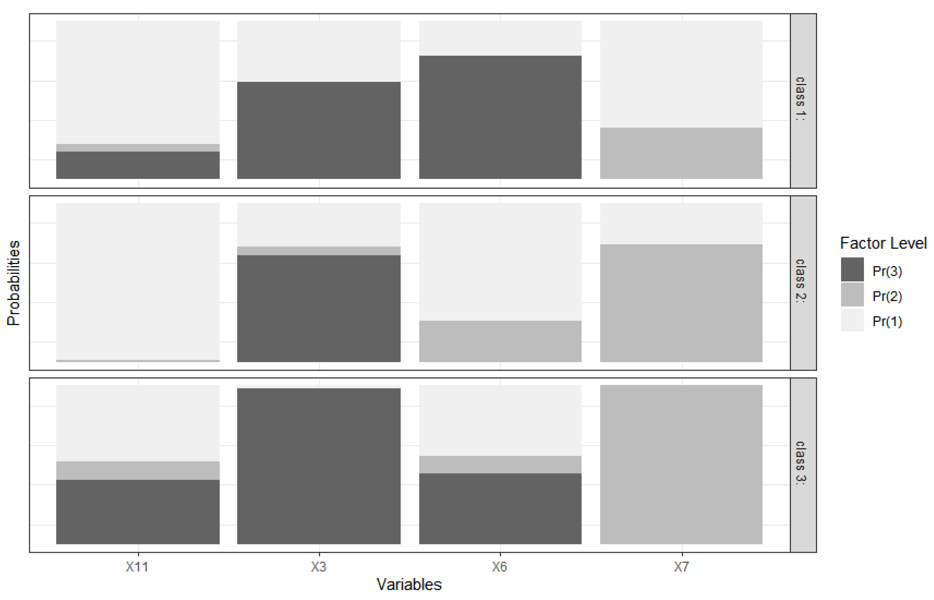
3.2. Application of Data

The Indonesian government has determined the classification of villages into five groups, namely independent villages, developed villages, developing villages, underdeveloped villages, and very underdeveloped villages. Problems arise when one of the villages divides and sufficient data are needed to place the new villages resulting from the division into existing village groups. This study proposed MI-based variable selection on an LCC analysis for grouping villages with the aim of obtaining the minimum data requirements for the placement of the new village. The data used in this study were 2018 village-potential data from Banyumas Regency, which were obtained from a census that was conducted by Statistics Indonesia (Badan Pusat Statistik abbreviated as BPS). These data belong to the regional (spatial) data highlighting the potential of an area. This study intended to show the influence of the socio-economic sector on village grouping; therefore, we examined only data on village potential in the socio-economic sector. The twelve variables used are described in

Table 1. Description of variables.

Variable (n = 301)	Value	%
The main source of income for the majority of the population (X1)	1 = agriculture	75.53
	2 = non-agriculture	24.47
Cooking fuel for the majority of families in the village (X2)	1 = LPG gas	98.49
	2 = non-LPG gas	1.51
Temporary landfill (X3)	1 = yes, used	25.98
	2 = yes, not used	2.11
	3 = no	71.91
Toilet facility usage of the majority of families (X4)	1 = toilet	99.09
	2 = non-toilet	0.91
A final disposal site for the stool of the majority of families (X5)	1 = tank	71.60
	2 = non-tank	28.40
The existence of springs in the village (X6)	1 = yes, managed	49.85
	2 = yes, not managed	14.80
	3 = no	35.35
The existence of high schools and equivalent education institutions (X7)	1 = yes	28.70
	2 = no	71.30
The existence of health facilities (X8)	1 = yes	99.09
	2 = no	0.91
Extraordinary events or disease outbreaks in the past year (X9)	1 = yes	1.81
	2 = no	98.19
The widest type of road surface (X10)	1 = asphalt/concrete	99.70
	2 = others	0.30
The existence of public transportation (X11)	1 = yes, with fixed routes	75.53
	2 = yes, without fixed routes	6.04
	3 = no	18.43
The existence of residents who use handphones (X12)	1 = mostly residents	99.40
	2 = a small number of residents	0.60

.

Mutual information-based variable selection in LCC analysis is used as the first step in data application. The selection of variables begins by estimating several models used in the selection of variables in a number of different clusters. Vermunt and Magidson [19] suggested estimating the model up to a four-cluster model, but our study used the estimation of the model up to a ten-cluster model. This was performed to ensure that the selected variables were the best variables.

Table 2. Alternative models of mutual information-based variable selection in LCC analysis for village-potential data processing in village grouping.

Alternative Model	The Best Variables	Mutual Information
Model 2 (two-cluster)	X6; X8; X11	0.2538
Model 3 (three-cluster)	X3; X6; X11	0.2862
Model 4 (four-cluster)	X5; X6; X7; X11	0.3257
Model 5 (five-cluster)	X5; X6; X7; X11	0.4413
Model 6 (six-Cluster)	X3; X6; X7; X11	0.4561
Model 7 (seven-Cluster)	X3; X5; X6; X7; X11	0.4396
Model 8 (eight-Cluster)	X3; X5; X6; X7; X11	0.3956
Model 9 (nine-Cluster)	X3; X5; X6; X7; X11	0.4223
Model 10 (ten-Cluster)	X3; X5; X6; X7; X11	0.4440

shows the results of the selection of variables for two-cluster to ten-cluster models, along with their mutual information values. The mutual information (MI) in Table 2 shows that the combination of variables in Model 6 (i.e., six-clusters) was the most suitable combination of variables among other models, because Model 6 had the largest MI value of 0.4561. Mutual information-based variable selection using Model 6 (six-clusters) resulted in variables X₃, X₆, X₇, and X₁₁.

The four selected variables corresponded to several village sustainable development goal (SDG) indicators [28]. The corresponding village SDG indicators were as follows:

• Temporary landfill (X₃) was representative of village SDG indicator number 12: environmentally aware village consumption and production.
• The existence of springs in the village (X₆) was representative for village SDG indicator number 6: villages with clean water and sanitation.
• The existence of high schools and equivalent education institutions (X₇) was representative of the village SDG indicator number 4: quality village education
• The existence of public transportation (X₁₁) was representative of village SDG indicator number 9: village infrastructure and innovation according to needs.

The selected variables above were associated with the village SDGs because the 11 sustainable national development goals were closely related to village territory. Due to this, the Indonesian government launched the village SDGs. In general, the village SDGs have contributed to the SDGs.

The selected variables were used as the basis for collecting data for the new villages resulting from the division. Consequently, assignment of the new villages into the existing groups could be simplified by using only the data based on the selected variables. Thus, variable selection could speed up time, reduce costs, and reduce energy required to provide data. This was very beneficial for local governments (especially new villages resulting from the division) because fewer variables were needed.

The accuracy of the new village placement can be seen from the results of grouping villages based on LCC analysis using selected variables compared to all variables. This comparison is explained in the following discussion.

Furthermore, the four selected variables (X₃, X₆, X₇, X₁₁) were modelled using LCC analysis.

Table 3. Final alternative model formed from village-potential data processing in village grouping using LCC analysis.

Alternative Model	Log- Likelihood	AIC	BIC	Adjusted BIC	Number of Parameters
Model 2 (two-cluster)	−837.390	1704.780	1760.386	1712.815	15
Model 3 (three-cluster)	−821.723	1689.445	1774.709	1701.766	23
Model 4 (four-cluster)	−817.460	1696.920	1811.841	1713.526	31
Model 5 (five-cluster)	−813.988	1705.976	1850.554	1726.868	39
Model 6 (six-cluster)	−812.992	1719.985	1894.219	1745.162	47
Model 7 (seven-cluster)	−812.620	1735.239	1939.130	1764.701	55
Model 8 (eight-cluster)	−812.620	1751.239	1984.787	1784.987	63
Model 9 (nine-cluster)	−812.620	1767.239	2030.444	1805.282	71
Model 10 (ten-cluster)	−812.096	1782.193	2075.054	1824.511	79

describes the results of grouping villages with the selected variables for the two-cluster to ten-cluster models. Model 3 (three-cluster) presented the lowest AIC and adjusted BIC values; however, Model 2 (two-cluster) presented the lowest estimate for BIC. Therefore, Model 3 was chosen as the optimal model considering that the adjusted BIC value is the most accurate information criterion, as recommended by Yang [29]. From the explanation above, it can be concluded that the selected number of clusters was a model with three latent classes. The complete comparison of the model after the variable selection is shown in Table 3, while the item response probabilities for each variable are shown in Figure 1. In general, the result of this clustering was that 95 villages were members of the first cluster, 166 villages were members of the second cluster, and 40 villages were members of the third cluster. The ranking of villages according to the socio-economic aspects of villages in 2018 in Banyumas Regency can be concluded as follows:

• A total of 40 villages that were members of Cluster 1 were included in the independent village qualifications (rank 1);
• A total of 95 villages that were members of Cluster 2 were included in the advanced village qualifications (rank 2);
• A total of 166 villages belonging to Cluster 3 were included in the qualification for developing villages (rank 3).

Riyanto et al. [30] performed village clustering using all variables from these research data with LCC analysis and obtained a three-cluster model. The study showed that as many as 39 villages were included in Cluster 1, 90 villages were included in Cluster 2, and 172 villages were included in Cluster 3. Meanwhile, in this research, 40 villages were included in Cluster 1, 95 villages were included in Cluster 2, and 166 villages were included in Cluster 3. The comparison of the results of grouping with LCC analysis between all these variables and the four selected variables in this study is presented in

Table 4. The comparison of clustering results between all variables and the four selected variables.

The Four Selected Variables	All Variables			Sum
	Cluster 1	Cluster 2	Cluster 3
Cluster 1	37	2	1	40
Cluster 2	2	88	5	95
Cluster 3	0	0	166	166
Sum	39	90	172	301

. The grouping of villages using the four selected variables in this study resulted in 10 villages whose grouping did not match that of the grouping obtained using all of the variables. From Table 4, we can calculate the accuracy level of this grouping, which was 96.678%. This shows that variable selection provided selected variables that could describe the original variable (all variables before selection).

4. Conclusions

We introduced the MI-based variable-selection method, which could be used for clustering villages with LCC analysis. In its application, the results of this variable selection can be used by local governments to make it easier to classify new villages resulting from division. There are not usually enough data to classify new villages resulting from division. In order to speed up the collection of the data used in clustering, it was necessary to simplify the collected data. This was achieved by means of MI-based variable selection. The application of this method used 2018 village-potential data for Banyumas Regency. The variable selection carried out resulted in four variables (temporary landfill, the existence of springs in the village, the existence of high schools and equivalent educational institutions, and the existence of public transportation), which were then used for village grouping using LCC analysis. Using the results of the analysis with the LCC analysis, the villages were grouped into three clusters. The clustering accuracy rate achieved from the results of this variable selection was 96.678%, compared to clustering using the original data.

This study is more focused on the selection of variables whose results are used in placing new objects into existing groups, so there are still some limitations. These limitations include only considering MI in the selection of variables and not comparing it with other variable selection methods. In addition, this study also used a forward search procedure in the variable selection process. As consideration for further research, measures other than MI can be added to the variable selection process, compared with other variable selection methods, and using other search procedures that could produce better models.

References

1. Liu, H.; Yu, L. Toward Integrating Feature Selection Algorithms for Classification and Clustering. IEEE Trans. Knowl. Data Eng. 2005, 17, 491–502. [Google Scholar]
2. Kim, Y.S.; Steet, W.N.; Menczer, F. Feature Selection in Unsupervised Learning via Evolutionary Search. In Proceedings of the Sixth ACM SIGKDD International Conference Knowledge Discovery and Data Mining, Boston, MA, USA, 20–23 August 2000; pp. 365–369. [Google Scholar]
3. Dash, M.; Choi, K.; Scheuermann, P.; Liu, H. Feature Selection for Clustering—A Filter Solution. In Proceedings of the Second International Conference Data Mining, Maebashi City, Japan, 9–12 December 2002; pp. 115–122. [Google Scholar]
4. Vergara, J.R.; Estevez, P.A. A Review of Feature Selection Methods Based on mutual Information. Neural Comput. Appl. 2014, 24, 175–186. [Google Scholar] [CrossRef]
5. Hall, M.A. Correlation Based Feature Selection for Discrete and Numeric Class Machine Learning. In Proceedings of the 17th International Conference Machine Learning, Standord, CA, USA, 29 June–2 July 2000; pp. 359–366. [Google Scholar]
6. Liu, H.; Setiono, R. A Probabilistic Approach to Feature Selection—A Filter Solution. In Proceedings of the 13th International Conference Machine Learning, Bari, Italy, 3–6 July 1996. [Google Scholar]
7. Yu, L.; Liu, H. Feature Selection for High-Dimensional Data: A Fast Correlation-Based Filter Solution. In Proceedings of the 20th International Conference Machine Learning, Washington, DC, USA, 21–24 August 2003; pp. 856–863. [Google Scholar]
8. Caruana, R.; Freitag, D. Greedy Attribute Selection. In Proceedings of the 11th International Conference Machine Learning, New Brunswick, NJ, USA, 10–13 July 1994; pp. 28–36. [Google Scholar]
9. Dy, J.G.; Brodley, C.E. Feature Subset Selection and Order Identification for Unsupervised Learning. In Proceedings of the 17th International Conference Machine Learning, Standord, CA, USA, 29 June–2 July 2000; pp. 247–254. [Google Scholar]
10. Kohavi, R.; John, G.H. Wrappers for Feature Subset Selection. Artif. Intell. 1997, 97, 273–324. [Google Scholar] [CrossRef] [Green Version]
11. Das, S. Filters, Wrappers and a Boosting-Based Hybrid for Feature Selection. In Proceedings of the 18th International Conference Machine Learning, San Francisco, CA, USA, 28 June–1 July 2001; pp. 74–81. [Google Scholar]
12. Ng, A.Y. On Feature Selection: Learning with Exponentially Many Irrelevant Feature as Training Examples. In Proceedings of the 15th International Conference Machine Learning, Madison, WI, USA, 24–27 July 1998; pp. 404–412. [Google Scholar]
13. Xing, E.; Jordan, M.; Karp, R. Feature Selection for High-Dimensional Genomic Microarray Data. In Proceedings of the 15th International Conference Machine Learning, Williamstown, MA, USA, 18–24 July 2001; pp. 601–608. [Google Scholar]
14. Venkatesh, B.; Anuradha, J. A Review of Feature Selection and Its Methods. Cybern. Inf. Technol. 2019, 19, 3–26. [Google Scholar] [CrossRef] [Green Version]
15. Leung, Y.; Hung, Y. A Multiple-Filter-Multiple-Wrapper Approach to Gene Selection and Microarray Data Classification. IEEE/ACM Trans. Comput. Biol. Bioinform. 2010, 7, 108–117. [Google Scholar] [CrossRef] [PubMed] [Green Version]
16. Lazar, C.; Taminau, J.; Meganck, S.; Steenhoff, D.; Coletta, A.; Molter, C.; Nowe, A. A Survey on Filter Techniques for Feature Selection in Gene Expression Microarray Analysis. IEEE/ACM Trans. Comput. Biol. Bioinform. 2012, 9, 1106–1119. [Google Scholar] [CrossRef] [PubMed]
17. Shen, Q.; Diao, R.; Su, P. Feature Selection Ensemble. Turing-100 2012, 10, 289–306. [Google Scholar]
18. Gutkin, M.; Shamir, R.; Dror, G. SlimPLS: A Method for Feature Selection in Gene Expression-Based Disease Classification. PLoS ONE 2009, 4, e6416. [Google Scholar] [CrossRef] [PubMed] [Green Version]
19. Vermunt, J.K.; Magidson, J. Latent Class Analysis. In The Sage Encyclopedia of Social Science Research Methods; Lewis-Beck, M.S., Liao, T.F., Eds.; SAGE Publications, Inc.: New York, NY, USA, 2004. [Google Scholar]
20. Vermunt, J.K.; Magidson, J. Latent Class Models for Clustering: A Comparison with K-Means. Can. J. Mark. Res. 2002, 20, 36–43. [Google Scholar]
21. Dempster, A.P.; Laird, N.M.; Rubin, D.B. Maximum Likelihood from Incomplete Data via the EM Algorithm. J. R. Stat. Soc. Ser. B (Methodol.) 1977, 39, 1–38. [Google Scholar]
22. Sclove, L. Application of Model-Selection Criteria to Some Problems in Multivariate Analysis. Psychometrika 1987, 52, 333–343. [Google Scholar] [CrossRef]
23. Schwartz, G. Estimating the Dimension of a Model. Ann. Stat. 1978, 6, 461–464. [Google Scholar] [CrossRef]
24. Battiti, R. Using Mutual Information for Selecting Feature in Supervised Neural Net Learning. IEEE Trans. Neural Netw. 1994, 5, 537–550. [Google Scholar] [CrossRef] [PubMed] [Green Version]
25. Fleurit, F. Fast binary Feature Selection with Conditional Mutual Information. J. Mach. Learn. Res. 2004, 5, 1531–1555. [Google Scholar]
26. Doquire, G.; Verleysen, M. An Hybrid Approach to Feature Selection for Mixed Categorical and Continuous Data. In Proceedings of the International Conference on Knowledge Discovery and Information Retrieval, Paris, France, 26–29 October 2011; pp. 386–393. [Google Scholar]
27. Gomez-Verdejo, V.; Verleysen, M.; Fleury, J. Information Theoretic Feature Selection for Function Data Classification. Neurocomputing 2009, 72, 3580–3589. [Google Scholar] [CrossRef]
28. Tenaga Pendamping Profesional Pusat. Pendataan SDG’s Desa 2021; Kemendesa PDT dan Trnasmigrasi: Jakarta, Indonesia, 2021. [Google Scholar]
29. Yang, C. Evaluating Latent Class Analysis Models in Qualitative Phenotype Identification. Comput. Stat. Data Anal. 2006, 50, 1090–1104. [Google Scholar] [CrossRef]
30. Riyanto, A.; Kuswanto, H.; Prastyo, D.D. Latent Class Cluster for Clustering Villages Based on Socio-Economic Indicators in 2018. J. Phys. Conf. Ser. 2021, 1821, 012041. [Google Scholar] [CrossRef]
Figure 1. Item response probabilities.
Symmetry 14 00908 g001