Article

DII-GCN: Dropedge Based Deep Graph Convolutional Networks

1
School of Computer Science and Mathematics, Fujian University of Technology, Fuzhou 350118, China
2
School of Computer Science and Information Engineering, Harbin Normal University, Harbin 150080, China
*
Author to whom correspondence should be addressed.
Symmetry 2022, 14(4), 798; https://doi.org/10.3390/sym14040798
Submission received: 7 March 2022 / Revised: 31 March 2022 / Accepted: 8 April 2022 / Published: 12 April 2022
(This article belongs to the Special Issue Recent Advances in Granular Computing for Intelligent Data Analysis)

Abstract

:
Graph neural networks (GNNs) have gradually become an important research branch in graph learning since 2005, and the most active one is unquestionably graph convolutional neural networks (GCNs). Although convolutional neural networks have successfully learned for images, voices, and texts, over-smoothing remains a significant obstacle for non-grid graphs. In particular, because of the over-smoothing problem, most existing GCNs are only effective below four layers. This work proposes a novel GCN named DII-GCN that originally integrates Dropedge, Initial residual, and Identity mapping methods into traditional GCNs for mitigating over-smoothing. In the first step of the DII-GCN, the Dropedge increases the diversity of learning sample data and slows down the network’s learning speed to improve learning accuracy and reduce over-fitting. The initial residual is embedded into the convolutional learning units under the identity mapping in the second step, which extends the learning path and thus weakens the over-smoothing issue in the learning process. The experimental results show that the proposed DII-GCN achieves the purpose of constructing deep GCNs and obtains better accuracy than existing shallow networks. DII-GCN model has the highest 84.6% accuracy at 128 layers of the Cora dataset, highest 72.5% accuracy at 32 layers of the Citeseer dataset, highest 79.7% accuracy at 32 layers of the Pubmed dataset.

1. Introduction

Graphs are intuitive expressions that describe objects and their relationships. Graph data based on graph structures are ubiquitous in the real world and have powerful representation capabilities. Therefore, it has become an important data source for learning [1]. Graph data has the following characteristics: (1) Node features: the attributes of the node itself, the feature set that needs to be paid attention to as the observation object. (2) Structural features: the topological structure between nodes in the graph data described by the edges between nodes. Graph data analysis has a wide range of application values, such as graph classification tasks [2], graph image structure reasoning [3,4,5,6,7,8].
Because of the success of deep neural networks, Graph Neural Networks (GNNs) have been applied in graph data analysis and have become an important research branch. As a landmark achievement of the third wave of artificial intelligence, deep learning has made essential breakthroughs in image and speech analysis applications. However, the most popular convolutional neural networks (CNNs) are still pondering and solving problems in the traditional Euclidean space.
As shown in Figure 1, traditional CNNs independently employ the observed objects as input for iterative analysis, ignoring the relationship between the objects. GNN can directly analyze the object’s structure as input in recent years, which breaks the Euclidean space limitation of traditional image processing and shows enormous potential demand.
Compared to CNNs, GNNs are more visible in explaining object relationships, the human thinking prototype, and a broader spectrum of applications, although it is still in development. GCNs [9] face challenges in the effectiveness of crucial convolution kernels and pooling operations. Nowadays, the fundamental concern that plagues GCNs is the phenomenon of over-smoothing [10]. The original GCN model has only two layers [11]. When the depth deepens, the GCN model ability effect will worsen [12,13]. The over-smoothing has evolved into a major obstacle in the development of GCN. The portion reason is that the graph data structure does not constrain the spatial translation of the lattice image. After multi-layer Laplace transform, the most eigenvalues of the nodes in the graph can rapidly reach a particular fixed smoothing value. The reason is not that fast Laplace smoothing is in GCN, but that immediate smoothing leads to tuning. As a result, the space becomes narrow, making it difficult to achieve fine-grained learning and continuously improve the performance of the GCN model.
Research on improving the representation capability of GCNs by deepening the network hierarchy has received considerable attention [14,15]. Chen et al. proposed GCNII, which achieved the smooth connection of cross-layer by adding initial input information in identity connections learning. In addition, one of the successful works that jump cross-layer to realize the deep GCN is Jumping Knowledge Network (JKNet) [15]. The JKNet model proposed an adaptive selective aggregation mechanism, which utilized cross-layer jump links to unite the shallow feature into the deep layer so that each node can adaptively adjust aggregation radius, effectively avoiding the semantic deviation caused by the over-smoothing. Both GCNII and JKNet are effective attempts that made the model in deep GCN. Hence, it is foreseeable that the deep GNN will be an essential research direction in the future.
GCN nature is feature aggregation. The learning purpose is to find the state of aggregation convergence. When the convergence outcome is consistent with the domain semantics, it is successful learning. GCN input is a richer information graph structure. It is not only considered the nodes but also edges, the repeated usage of adjacent node features speeds up the GCN convergence rate, and it is easy to produce excessive smoothness. Cutting the input graph data increase GCN generalization ability and enhances semantic scalability, preventing extreme smoothing. There are three paths for cutting GCN: Cut output (DropOut) [16], Cut point (DropNode) [17], and Cut Edge (Dropedge) [9]. Cut output appropriately crop the output value of the hidden layer node, which makes output less than the next layer. Cut output has been proposed in ordinary deep neural networks and has been broadly adopted [18]. The clipping point implies clipping the node in the input graph, and the clipping edge conveys clipping the edge in the input graph. The clipping point is stronger than the clipping edge because cutting a node not only the corresponding entity but also the edges that exist and are attached to a node. Several explorations have proved that the cutting point method is difficult to control, and the cutting edge may be more suitable for the GCN network. The corresponding experiment also confirmed that GCN employed Dropedge [9] could delay the occurrence of over-smoothing and make it possible to construct deep GCN. This paper aims to dissect the elements that hinder deeper GCNs from carrying out likely and exploit mediums to address the problem.
The significant contributions of this work are twofold. First, we propose a novel model called DII-GCN by integrating residual convolution, identity mapping, and Dropedge techniques. Second, we conducted comparative experiments on standard datasets comprising Cora, Citeseer, and Pubmed to validate the effectiveness.
The rest of this paper is organized as follows. Section 2 outlines the related works. In Section 3, we introduce the framework of DII-GCN. Section 4 conducts experiments and analytical outcomes compared with other existing algorithms. We provide conclusions and future work in Section 5.

2. Related Works

Gori et al. were the first to pay attention to graph data processing and proposed the GNN model, which realizes an action that maps a graph and one of its intersections into a spatial Euclidean space [19]. Gori draws on the ordinary neural network structure to process graph structure data directly. Therefore, this model can be considered as a GNN. The groundbreaking network laid the foundation for the development of subsequent GNNs. In 2013, Bruna et al. employed Laplacian and Fourier transform techniques to solve the graph data convolution calculation and proposed the first GCN. Tentative shows that low spatial graphs are probable to be trained convolutional layers with parameters numbers alone of the input measurement, resulting in prompt deep structure [20]. In 2016, Kipf and Welling utilized the thought of first-order neighbor aggregation and proposed the GCN model [11], which was used as the basic GCN model in most subsequent studies.
The GCNs model’s optimal performance proposed by Kipf and Welling is only two layers. It confirmed that this GCN model is unsuitable for building a deep network. Deepening the model depth will lead to a sharp decline in the aggregation effect. Another successful result found that moderate a Dropedge of graph structure data can solve the GCN over-smoothing problem. Deleting some edges of the input graph data alters the connection between nodes to a certain extent, differentiating the aggregation of nodes and enhancing the diversity of training data. The model generalization ability is improved.
In recent years, the application of graph data has become a popular research direction. For example, Guo applied GCN to dynamic network anomaly detection, which enhanced an unsupervised graph neural network skeleton called DGI, which mutually collects the unusual features of the network oneself [21]. Wang used the GCN network to realize human pose estimation exploits Global Nexus Inference Graph Convolutional Networks to catch the global connection among distinct body joints quickly [22]. Yu operated GCN to solve the rumor detection problem in social networks, which shows the affection architecture of tattle with a graph convolution operator for node vector updating [23]. Wu proposed a new taxonomy to partition the graph neural networks into four classifications by extracting the evaluation of GNN models [24]. BI applied a model that combines GNN and CNN to resolve the Knowledge based completion task, and the model has learnable weights that fit based on the message from vicinage and can use accessorial knowledge for out-of-knowledge-base entities to calculate their mosaic. At the same time, the remaining parameter was prompt [25]. Sichao used two-order GCN for semi-supervised classification. The two-order polynomial in the Laplacian can assimilate much-localized structure information of graph data and then boost the classification significantly [26]. Chen employed augmented normalized Laplacian spectrum in weight array to deal with more non-linearities [27]. Cai suggests two taxonomies of graph embedding in different graph issues [28]. Petar reveals graph attention networks, heaping up layers in which nodes are capable of looking after neighborhoods features. Meanwhile, address some crux challenges of spectral-based graph neural networks, and make the model readily applicable to inductive and transductive issues [29].
The particular GCN models include: JKNet, SpectralGCN [20], ChebNets, CayleyNets, SpectralGCN etc. ChebNets show the capability of this deep learning system to train local, stationary, and ingredient aspects on graphs [30]. CayleyNets parametric reasonable complex functions (Cayley polynomials) permit computing efficiently spectral filters on graphs that specialize in frequency area generate spectral filters that are localized in airspace, scales linearly with the size of the input data for scattered congregate graphs [31]. Bruna constructed a spectral-based graph convolutional neural network (SpectralGCN), which provided a basis for subsequent research on spectral-based GCNs. Based on the SpectralGCN model, Defferrard proposed a ChebNets model that uses a K-degree polynomial filter in the convolutional layer. ChebNets aggregate K-order domain nodes and the computational performance is guaranteed. In 2017, Levie proposed a CayleyNets model based on the spectral method, which builds spectral convolution filters based on Cayley polynomials, improving learning accuracy from the SpectralGCN.

3. Preliminary

In this section, some terms related to GCN are described briefly first, which are the basis of our proposed model- DII-GCN.
A graph is an ordered pair G = ( V , E ) . Where V is a set of vertices (also called nodes or points), E { { x , y } x , y V and x y } represents a set of edges, which are unordered pairs of vertices (that is, an edge is associated with two distinct vertices). In particular, unlike CNN, the input of GCN is the self-graph.
For a simple graph with vertex set V = { v 1 , , v n } , the adjacency matrix is a square n × n matrix A such that its element A i j is one when there is an edge from vertex v i to vertex u j , and zero when there is no edge.
For above, G = ( V , E ) with | V | = n , the degree matrix D for G is a n × n diagonal matrix defined as follows.
D i , j : = deg ( v i ) i f i = j , 0 otherwise .
where the degree deg ( v i ) of a vertex counts the number of times an edge terminates at that vertex.
An identity matrix is a given square matrix of any order which contains on its main diagonal elements with a value of one. In contrast, the rest of the matrix elements are equal to zero. The n × n identity matrix, denoted I n , is a matrix with n rows and n columns. The entries on the diagonal from the upper left to the bottom right are all 1’s, and all other entries are 0.
Given a simple graph G with n vertices, its Laplacian matrix L n × n is given by: L = D A , where D is the degree matrix, and A is the graph’s adjacency matrix. Since G is a simple graph, A only contains 1 s or 0 s and its diagonal elements are all 0 s. In the case of directed graphs, either the indegree or outdegree might be used, depending on the application. The basic GCN is constructed on the Spectral-domain; the core is the Laplacian matrix calculation.
Before using the Laplacian matrix, the GCN uses two small tricks to improve performance: (1) Add a self-loop for all nodes to ensure self nodes and neighbor nodes participate in reasoning, this paper recorded as A); (2) Normalize to prevent gradient explosion or disappearance.
Definition 1
(Applicable Laplacian matrix). Given a graph G with added self-loops, the adjacency matrix A, degree matrix D, and identity matrix I, respectively. An applicable Laplacian matrix normalization method is given by:
L ^ = D 1 / 2 L D 1 / 2 = D 1 / 2 D D 1 / 2 D 1 / 2 A D 1 / 2 = I D 1 / 2 A D 1 / 2
L ^ is Symmetric-normalized Laplacian. Assume that A ^ = D 1 / 2 A D 1 / 2 , then A ^ that is a suitable operation unit, is used as the inference basis by most GCN models.
Definition 2
(Fourier transform of Laplacian matrix). Given a directed graph G, the eigenvalues and corresponding eigenvectors of Laplacian matrix L are given by,
= [ λ 1 , λ 2 , , λ n ] ( λ 1 λ 2 λ n ) , U = [ u 1 , u 2 , , u n ] .
For any signal on G, x ∈ R n , Fourier transform can be defined by x ¯ = f ( x ) = U T x ¯ .
Convolution based on spectral-domain analysis is completed in the Fourier domain. Therefore, relying on the Fourier transform and inverse Fourier transform by Definition 2, we can imitate the CNN convolution method to complete the graph convolution calculation.
Definition 3
(Simplified graph convolution). The convolution formula of a simplified GCN model can be defined by:
H l + 1 = f ( H l , A ^ ) = σ ( a ^ , H l , W l ) ,
where A ^ = D 1 / 2 A D 1 / 2 (A contains self-loop), W ( l ) is the learning weight of layer l, σ ( . ) is an activation function, respectively.
Convolution based on spectral-domain analysis is generally completed in the Fourier domain. Therefore, relying on the Fourier transform and inverse Fourier transform by Definition 2, we can imitate the CNN convolution method to complete the graph convolution calculation.
Definition 4
(Gradient in GCN). For a graph G, e i j is an edge from node v i to v j in G, and A = a i j , D = d i j are the adjacency matrix and degree matrix of G, respectively. Suppose J R n , an n-dimensional vector on G, then the e i j edge derivative at the v i node is calculated as follows:
J / e i j | i = a i j ( J i / d i i J j / d j j )
The node-related gradient is given by:
i = e i j G i ( J / e i j ) | i ) 2

4. Proposed Model

In this section, we propose the DII-GCN framework that integrates Dropedge, Initial residual, and Identity mapping methods into traditional GCNs.

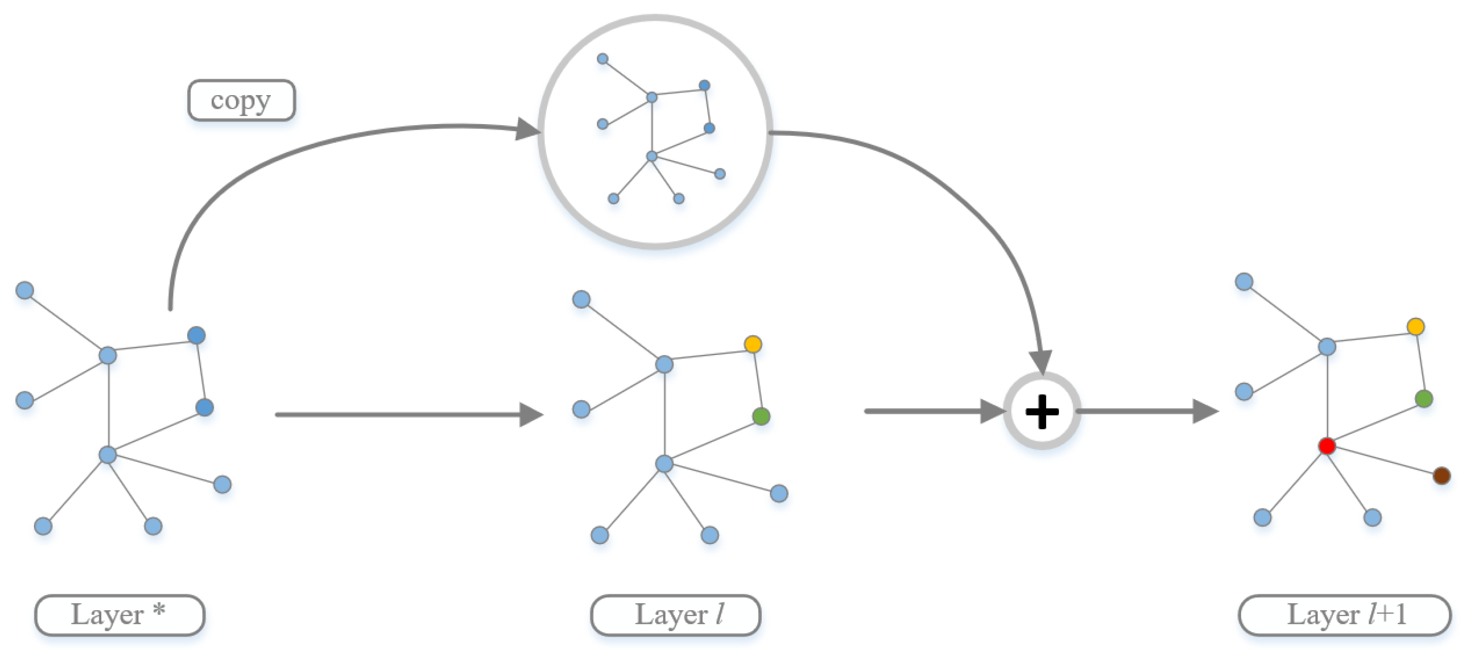
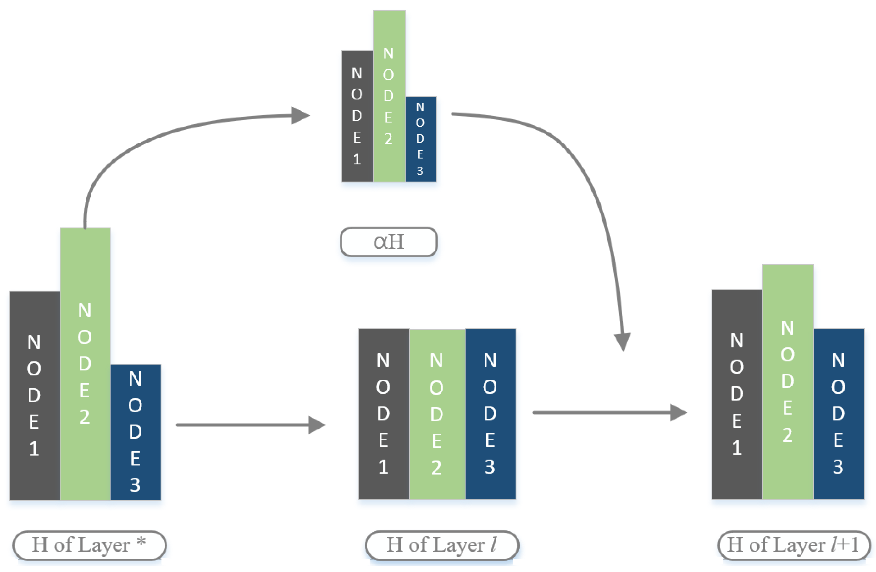
4.1. Residual Network and Cross-Layer Connection

The graph convolution model with residuals mainly introduces a shallow to deep jump link in a residual unit. For example, as shown in Figure 2, for the l + 1 layer, let the l layer output act as input. Adding (layer l) for the previous jump link prevents the spread of calculation deviations and improves aggregation performance.
Definition 5
(Graph convolution with residuals). The basic convolution formula of a GCN model with residuals is defined by:
H ( l + 1 ) = α H ( * ) + f ( H ( l ) , A ^ ) ,
where H ( * ) represents layer l, or the output of more shallow level.
The motivation for introducing residuals is to prevent the problem of gradient disappearance. Recent studies have also found that introducing GCN residuals for convolution calculation can strengthen the information complementarity between deep and shallow layers. In addition, introducing residual into a convolution network needs an identity mapping, which ensures the compatibility of shallow and deep layers of information and makes the network structure more uniform. Therefore, more conducive to improving the learning accuracy by deepening the network level.
The residual block is shown in Figure 2. There can be many ways to jump from the shallow to the deep layer, which must be considered in practical applications. For example, GCNII [14] uses the Initial residual method. Therefore, the initial input is connected to all the intermediate layer residual blocks. JKnet only selects the output of the last convolutional layer for fusion and aggregation. Thus, improving residual convolutional nets’ performance through cross-layer connections is currently one of the most explored methods, and it will continue to receive attention in the future. Figure 3 shows the principle of residual and identity mapping in GCN.
If the GCN network did not use a residual connection, the eigenvalues of the nodes would quickly become homogeneous (the parts of the l and l + 1 layers in Figure 3), the excessive smoothness phenomenon would occur. By adding a jump path from the shallow layer * to the deep layer l, the nodes of the l + 1 layer need to consider the comprehensive calculation results of layer l and layer *. Therefore, the shallow information is used to change the deviation in learning delays, over-smooth phenomenon and provides powerful support for the deep GCN.
Due to the identity mapping method, the node features effective superposition. Therefore, after several layers of GCN inference, identity mapping ensures each node is in the same dimension. The node features with residuals can be successfully introduced on the deep unit.

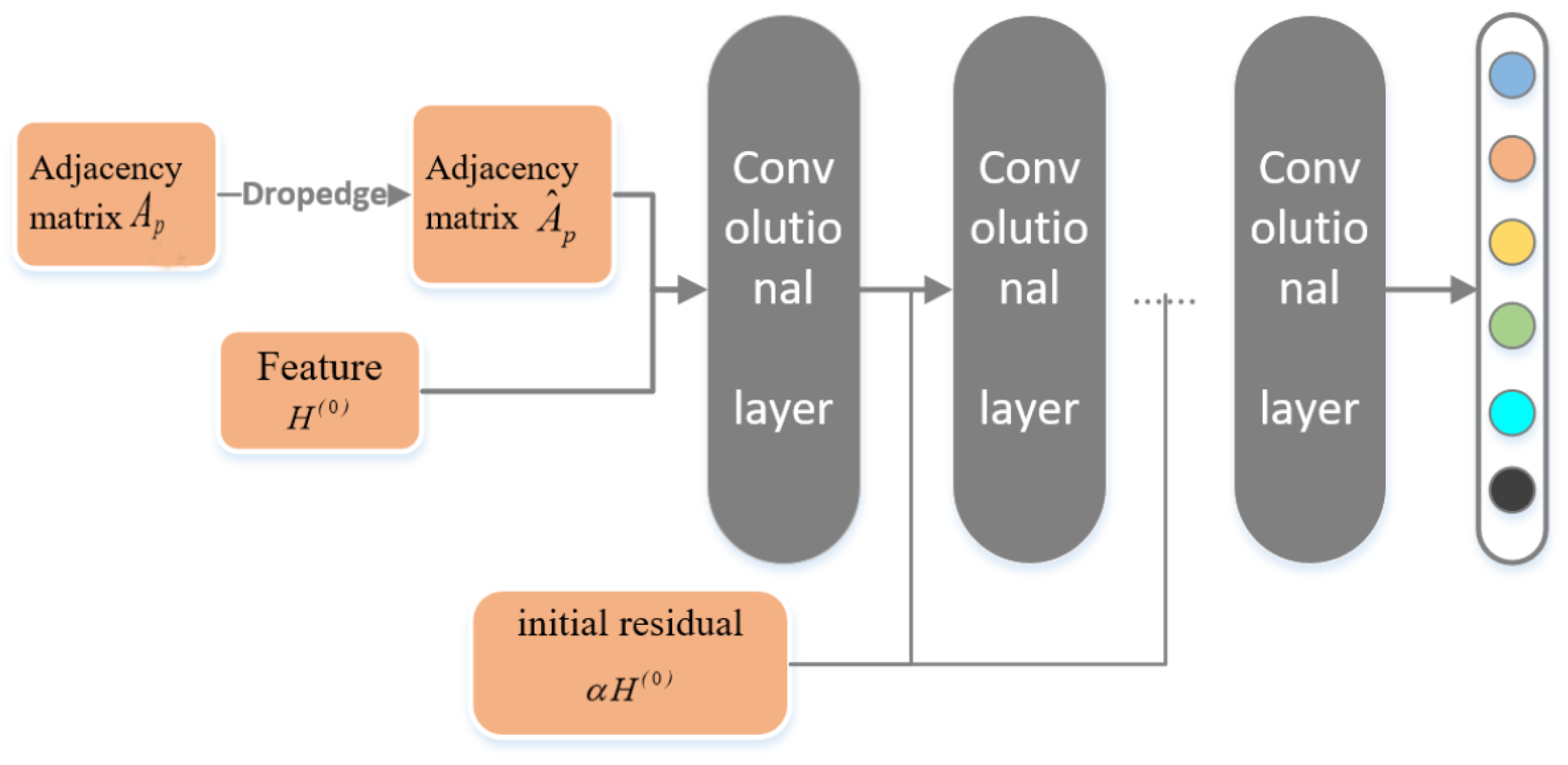
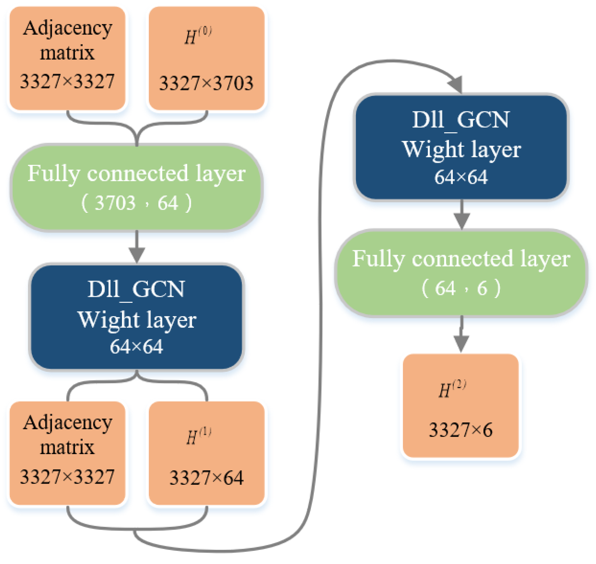
4.2. DII-GCN Model Design

Integrating graph Dropedge, initial network, identity mapping method, and the relevant definitions in the previous section, In this subsection, we propose a GNN model DII-GCN, as shown in Figure 4.
Dropedge has been proved to be an effective method for deep GCN, and its primary functions are summarized as follows. First, Dropedge can be regarded as a data enhancement method. The input adjacency matrix is randomly deleted during the training process, increasing the model’s input data diversity. Second, Dropedge method employed in training enhance the distinction between nodes, reducing information repetitive utilization, and slow down the over-smoothing phenomenon.
Definition 6
(Graph convolution of DII-GCN). For graph G, suppose the Dropedge probability is p, then we use A p to represent the normalized adjacency matrix after Dropedge:
H ( l + 1 ) = f ( H ( l ) , A ^ ) = σ ( ( 1 α ) A p ^ H l + α H ( 0 ) ( ( 1 β ) I + β W ( l ) ) ) .
where H ( l ) is the output vector of layer l, and l is the unit matrix.
Definition 6 shows that DII-GCN uses the initial residual H ( 0 ) . Experiments found that the initial residual is more effective.
Based on the initial residual and identity mapping, the l layer processing steps of the DII-GCN incorporating Dropedge operations are:
Step 1. Set the Dropedge coefficient p and randomly discard the edge according to the probability: A p ^ r e n o r m a l i z a t i o n ( A A ) .
Step 2. Set the control parameter α , import α to the initial input α H ( 0 ) .
Step 3. Fuse H ( l ) and H ( 0 ) to generate l l a y e r output with residuals: H * ( 1 α ) A p ^ H ( l ) + α H ( 0 ) .
Step 4. Set the control parameter β and implement identity mapping on the weight: W * ( 1 β ) I + β W l .
Step 5. Select the excitation function σ ,and generate layer l output: H ( l + 1 ) σ ( H * , W * ) .
A practical problem is setting the parameters p, α , β , and the excitation function σ in the DII-GCN model. Therefore, obtaining the optimized value is necessary according to the application background.
Experiment includes:
(1) p is the ratio of the preserved edges of the graph, the proportion of trimmed edges is 1 p , and the corresponding A p ^ is the regularized input matrix. However, p should not be too small because it will cause insufficient graph structural data and lose the advantage of the graph network; p should not be too large. It will make the data diversity inferior to the iterative process and produce excessive smoothing. The empirical p is between 0.7 and 0.9.
( 2 ) The parameter α that controls the initial residual should not be too large, generally set to 0.1 ~ 0.2 (Chen et al., 2020). However, as shown in Formula (6), a large α will directly weaken the upper layer calculation effect and seriously affect the learning efficiency.
( 3 ) Formula (6) uses ( 1 β ) I + β W ( l ) to replace the weight vector W ( l ) , which can ensure equivalent performance to the shallow model, conducive to cross-layer information aggregation. In other words, ( 1 β ) I + β W ( l ) is the regularized result of W ( l ) . Therefore, when β is small, the singular value of ( 1 β ) I + β W ( l ) will be close to 1 by setting the appropriate β value, that can achieve the balance between weight vector correction and network equivalence maintenance. It improved the system’s adaptability. In our experiment, β is set as a variable that changes with the layers l, the l o g ( λ / l + 1 ) λ is the control coefficient set to 0.5.
The primary structure of the 2-layer network learning process is analyzed by illustrating the DII-GCN basic principles. The dataset uses the standard data set Citeseer [32]. Figure 5 shows the processing of the 2-layer DII-GCN network process indication.
According to Figure 5, let p = 0.9 , α = 0.1 , and λ = 0.5 , the basic process of the 2-layer DII-GCN network processing in the Citeseer dataset is as follows:
(1) From the Citeseer dataset, obtain the input feature H ( 0 ) and the normalized adjacency matrix A p ^ after Dropedge. Dropedge sets a part adjacency matrix value to zero and does not change the adjacency matrix dimension.
(2) Through the fully connected layer of H 0 , the feature dimension becomes 64 to match the preset weight matrix W dimension, where the weight matrix is randomly generated. After the first DII-GCN convolutional layer, the intermediate feature vector H ( l ) is obtained.
(3) Input the updated H ( l ) and A p ^ to the next DII-GCN convolutional layer, and the fully connected layer, the final output feature vector H ( 2 ) is obtained. Formula (9) shows the final output H ( 2 ) and classification results after 100 network learning. Output = (3 0 1 …) of the classification results only shows that the first three nodes 1, 2, 3 are divided into the class identification of “3”, “0”, “1”. The specific way to obtain the position of the maximum of the corresponding row of the node in H ( 2 ) .
A ^ p = 0.153 0 0 0 0.2 0 0 0 0.5
H 2 = 2.462 2.148 1.916 0.823 ̲ 1.721 3.418 1.011 ̲ 1.808 3.147 3.978 2.431 1.131 2.439 0.846 ̲ 1.244 2.831 3.395 2.276

5. Experiment and Analysis

The experiment uses standard datasets, Cora, Citeseer, and Pubmed, for evaluation and comparison. All datasets are processed as undirected graphs, and the most significant connected part is considered. Each dataset corresponds to an undirected Connected graph. Table 1 gives the basic information of the three data sets in this experiment.
According to the current processing conventions of most work, we preprocess the three datasets with undirected graphs. Then datasets are used to evaluate and compare the model. Figure 6, Figure 7 and Figure 8 show the connected graphs of 3 datasets.

5.1. A Comparative Experiment of Learning and Classification Accuracy

The accuracy and precision in the experiment are calculated by Formulas (7) and (8):
A c c u r a c y = ( T P + T N ) / ( P + N )
P r e c i s i o n = T P / ( T P + F P )
The symbols corresponding to Formulas (7) and (8) are as follows:
(1)
P (Positive) and N (Negative): represent the number of positive and negative examples in the training sample, respectively.
(2)
TP (True Positives): The number of positive examples that are correctly classified. The number of samples that are positive and classified as positive by the model.
(3)
FP (False Positives): The number of positive examples incorrectly classified. The number of samples is negative but classified as positive by the classifier.
(4)
FN (False Negatives): The number of false negatives. The number of positive samples but classified as negative by the classifier.
(5)
TN (True negatives): The number of negative examples correctly classified. The number of negative samples is classified as negative one.
From Formulas (7) and (8), accuracy rate mainly reflects the learning effect of a learning method or algorithm; accuracy cares about classifying the positive example set and evaluated in a specific category. Therefore, it accurately reflects the impact of a particular category classification.
Formula (7) compares the accuracy in this paper. Table 2 shows the particular parameter settings in the comparison experiment. The parameters’ optimized values are obtained according to the model and the dataset’s characteristics.
According to the main methods used in this article, the comparison algorithm selected from the list: the basic GCN model (abbreviated as G), DropEdge method (abbreviated as D), and the initial residual method (abbreviated as R) with identity mapping:
(i)
Consider G separately. The typical algorithm GCN used in the experiment.
(ii)
Consider G+D. Rong (Rong et al., 2019) puts forward the reasons for Dropedge in GCN and demonstrates some effects. Therefore, we perfected G+D and named D-GCN for the comparative experiments in this paper.
(iii)
Consider G+R. GCNII is a typical representative model.
(iv)
Consider G+D+R. The DII-GCN model proposed in this paper belongs to this category.
The above four methods: GCN, D-GCN, GCNII, and the DII-GCN model, were selected and compared on the Cora, Citeseer, and Pubmed datasets. Table 3 shows the experimental results, and the underlined data has the highest accuracy, while the accuracy rate is the average value obtained from 100 experiments.
From Table 3:
(1)
The DII-GCN model has the highest accuracy on the three standard data sets.
(2)
The GCN model can obtain better learning accuracy on the 2-layer network. However, as the depth increases, the learning accuracy drops sharply, and not it is not easy to use the Dropedge method (corresponding to the G+D model) to support deep GCN construction.
(3)
The DII-GCN and GCNII models can support the construction of deep graph convolutional networks, and the learning accuracy of DII-GCN improved from GCNII on the three standard data sets.
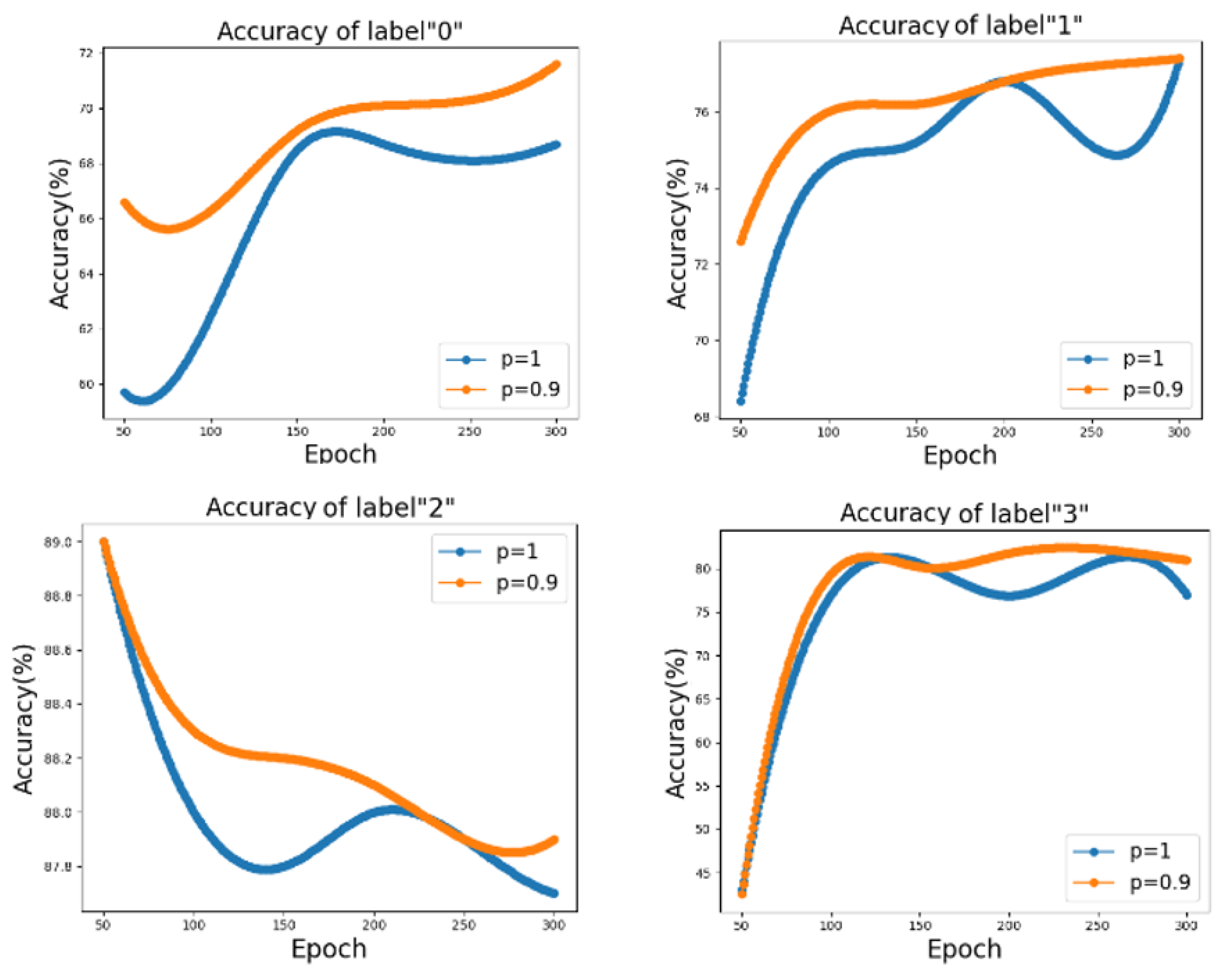
DII-GCN integrates the initial residual, identity mapping, and Dropedge method generally slows down the over-smoothing phenomenon and makes the information aggregation of the graph structure more refined. Specifically, the initial residual process superimposes the original node features in the deep model, the amplification or accumulation of node aggregation deviation prevented, and the life cycle of the network is prolonged. The identity mapping method enables the initial residual integrated into the deep convolution unit, ensuring the continued learning ability after the network is deepened. The Dropedge way further weakens the possibility of residual network degradation. Furthermore, through the change of graph structure data, the difference of the residual unit data input is increased, avoiding some nodes’ feature vectors assimilated in the adjacent residual layer. Therefore, the fineness of learning is improved.
In addition, Formula (8) carried out the classification accuracy of a single category. Figure 9 shows the accuracy changing for the Dropedge coefficient p is 1 and 0.9 on the Cora dataset based on the average value taken from 20 experiments. As shown in the Figure 9, the abscissa is a cycle of DLL-GCN network learning Times (epoch).
(1)
On the Cora dataset, for the first three classes (class identifiers are 0, 1, 2), the classification accuracy after Dropedge (p = 0.9) is better than the GNN without Dropedge (p = 1) at all iteration stages; For label 2, we found that the algorithm we proposed with other algorithms showed a decreasing trend in accuracy, but DII-GCN was still better than several others. The reason for their all decreasing may be the presence of numerous missing values in this category of data.
(2)
For class label 3, the previous Dropedge effect is not very satisfactory, but after 270 Epochs, the Dropedge appears to have a good effect. However, in a class with poor classification accuracy, the learning process improves by an appropriate number of iterations.

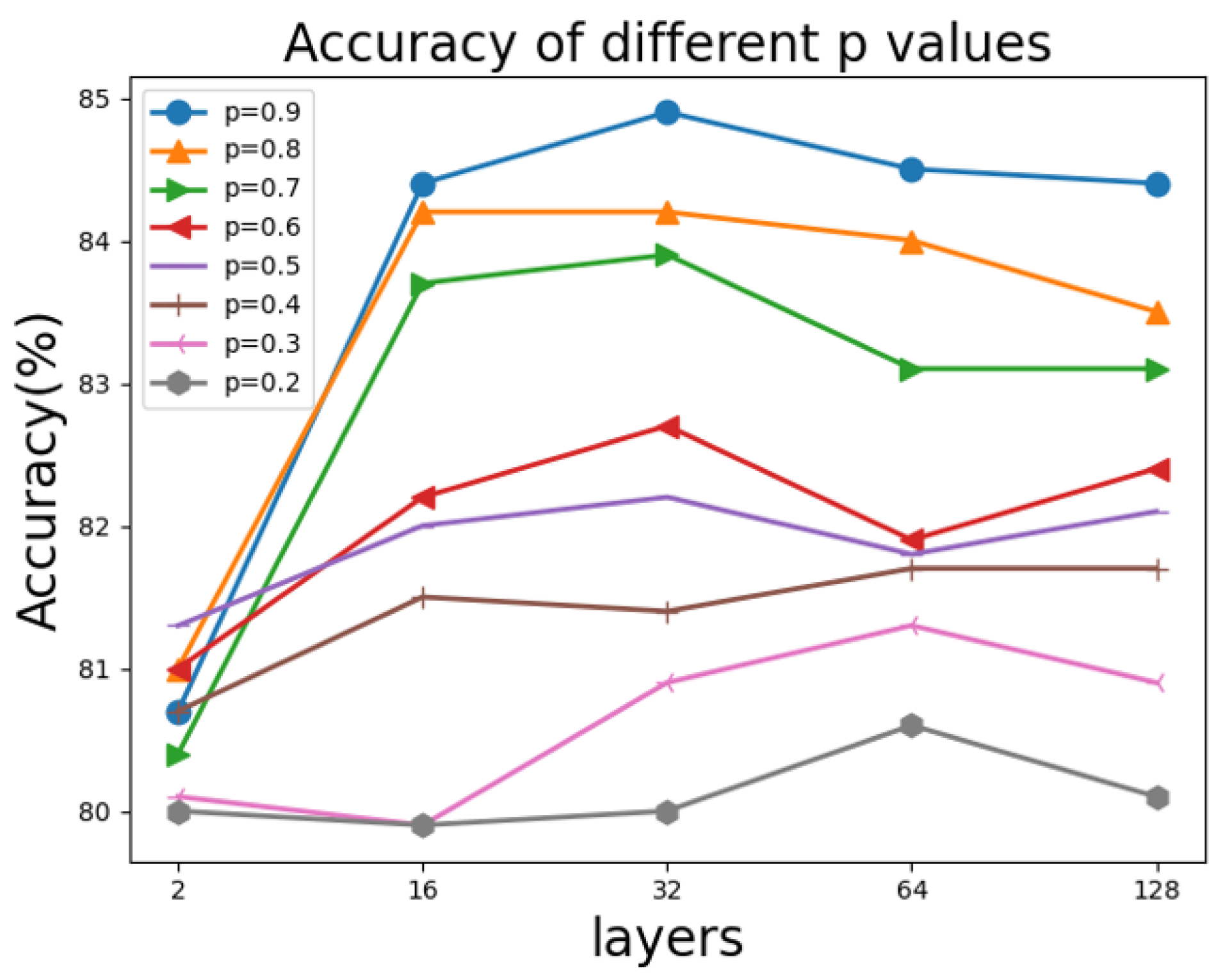
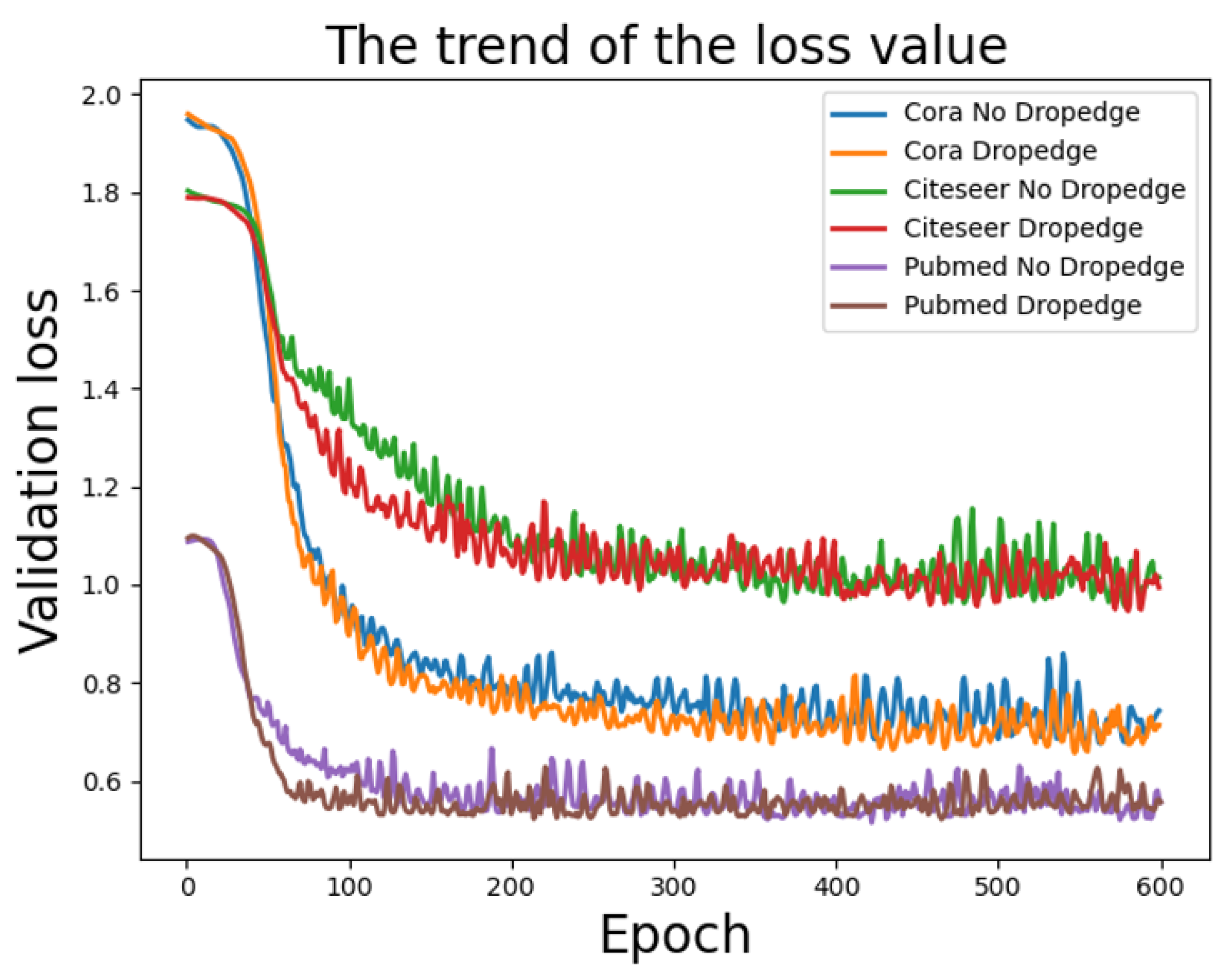
5.2. Dropedge Effectiveness Analysis

In order to explain the effectiveness of the Dropedge method on the model, we conduct an experiment with the Dropedge compared to DII-GCN by setting different layers and different p values. Figure 10 shows the corresponding p on the Cora dataset. The experiment result is an average of twenty times network learning.
(1)
For the Cora dataset, Dropedge coefficient p = 0.9 or 0.8, and the number of layers is over 16. Therefore, the DII-GCN model accuracy is around 84%. Furthermore, DII-GCN can deepen the network by setting the appropriate Dropedge coefficient p. As a result, the level can obtain a stable and higher learning accuracy.
(2)
When p is below 0.6, the DII-GCN model accuracy is not high, indicating the Dropedge effect is not ideal because too many Dropedges cause the graph data structure to be lost. It also illustrates the scientific meaning of the GNN. Using the associated information of the node can improve the node evaluation effect.
To intuitively convey the DII-GCN performance, we track the loss value (Val-loss) of the 4-layer DII-GCN model on the three standard datasets. Figure 11 shows the loss value trend of Dropedge (p = 0.9) and non-Dropedge (p = 1) as the number of training cycles increases.
Figure 11 shows that integrating the DII-GCN method can make the verification set loss value drop steadily and rapidly after 100 epochs, compared to non-Dropedge. DII-GCN method uses data diversity well and corrects deviations in the iterative process. It shows that the DII-GCN will not weaken the learning ability of the model.
In DII-GCN model, we have three steps, cut edges, initial residual, and Identity mapping. Comparing this proposed method with D_GCN, GCNII or GCN, the time complexity for aggregation reduces from O n 2 d ( l + 1 ) to O n ( d k ) ( l + 1 ) , where k is the number of cut edges. In terms of space complexity, graph convolutions in GCN formulations generally are O n 2 . DII-GCN is equivalent to the existing convolutions because it also provides a guaranteed space complexity of O ( n 2 ) .

6. Conclusions

In this work, we proposed DII-GCN that integrates Dropedge, Initial residual, and Identity mapping methods into traditional GCNs, directly oriented to the over-fitting and over-smoothing issues that need to be solved in the research of neural graph networks. Experimental results show that DII-GCN can increase the diversity of learning data and reduce the over-fitting phenomenon of training data. It can finely complete the information aggregation based on the graph structure and effectively prevent the over-smooth phenomenon, which provides an effective way to realize deep graph learning.
The DII-GCN model in this paper provides a new solution for constructing deep GCN networks, which effectively improves learning accuracy and classification accuracy on the standard dataset. Future work includes DII-GCN in the actual application scenario research, fusion of other technologies to improve further deep GNNs, etc.

Author Contributions

Conceptualization, methodology, writing—original draft preparation, J.Z. and G.M.; writing—review and editing, C.J. All authors have read and agreed to the published version of the manuscript.

Funding

This work was supported by the National Key Research and Development Plan of China (2019YFD0900805) and in part by the National Natural Science Foundation of China(61773415).

Institutional Review Board Statement

Not applicable.

Informed Consent Statement

Not applicable.

Data Availability Statement

Not applicable.

Conflicts of Interest

The authors declare no conflict of interest.

References

  1. Bo, B.; Yuting, L.; Chicheng, M.; Guanghui, W.; Guiying, Y.; Kai, Y.; Ming, Z.; Zhiheng, Z. Graph neural network. Sci. Sin. Math. 2020, 50, 367. [Google Scholar]
  2. Xinyi, Z.; Chen, L. Capsule graph neural network. In Proceedings of the International Conference on Learning Representations, Vancouver, BC, Canada, 30 April–3 May 2018. [Google Scholar]
  3. Gao, L.; Zhao, W.; Zhang, J.; Jiang, B. G2S: Semantic Segment Based Semantic Parsing for Question Answering over Knowledge Graph. Acta Electonica Sin. 2021, 49, 1132. [Google Scholar]
  4. Hamilton, W.L.; Ying, R.; Leskovec, J. Inductive representation learning on large graphs. In Proceedings of the 31st International Conference on Neural Information Processing Systems, Long Beach, CA, USA, 4–9 December 2017; pp. 1025–1035. [Google Scholar]
  5. Wang, X.; Ye, Y.; Gupta, A. Zero-shot recognition via semantic embeddings and knowledge graphs. In Proceedings of the IEEE Conference on Computer Vision and Pattern Recognition, Salt Lake City, UT, USA, 18–22 June 2018; pp. 6857–6866. [Google Scholar]
  6. Lin, W.; Ji, S.; Li, B. Adversarial attacks on link prediction algorithms based on graph neural networks. In Proceedings of the 15th ACM Asia Conference on Computer and Communications Security, Taipei, Taiwan, 5–9 October 2020; pp. 370–380. [Google Scholar]
  7. Che, X.B.; Kang, W.Q.; Deng, B.; Yang, K.H.; Li, J. A Prediction Model of SDN Routing Performance Based on Graph Neural Network. Acta Electonica Sin. 2021, 49, 484. [Google Scholar]
  8. Zitnik, M.; Agrawal, M.; Leskovec, J. Modeling polypharmacy side effects with graph convolutional networks. Bioinformatics 2018, 34, i457–i466. [Google Scholar] [CrossRef] [Green Version]
  9. Rong, Y.; Huang, W.; Xu, T.; Huang, J. Dropedge: Towards deep graph convolutional networks on node classification. arXiv 2019, arXiv:1907.10903. [Google Scholar]
  10. Perozzi, B.; Al-Rfou, R.; Skiena, S. Deepwalk: Online learning of social representations. In Proceedings of the 20th ACM SIGKDD International Conference on Knowledge Discovery and Data Mining, New York, NY, USA, 24–27 August 2014; pp. 701–710. [Google Scholar]
  11. Kipf, T.N.; Welling, M. Semi-supervised classification with graph convolutional networks. arXiv 2016, arXiv:1609.02907. [Google Scholar]
  12. Karpathy, A.; Toderici, G.; Shetty, S.; Leung, T.; Sukthankar, R.; Fei-Fei, L. Large-scale video classification with convolutional neural networks. In Proceedings of the IEEE Conference on Computer Vision and Pattern Recognition, Columbus, OH, USA, 23–28 June 2014; pp. 1725–1732. [Google Scholar]
  13. Long, J.; Shelhamer, E.; Darrell, T. Fully convolutional networks for semantic segmentation. In Proceedings of the IEEE Conference on Computer Vision and Pattern recognition, Boston, MA, USA, 7–12 June 2015; pp. 3431–3440. [Google Scholar]
  14. Chen, M.; Wei, Z.; Huang, Z.; Ding, B.; Li, Y. Simple and deep graph convolutional networks. In Proceedings of the International Conference on Machine Learning, PMLR, Online, 13–18 July 2020; pp. 1725–1735. [Google Scholar]
  15. Xu, K.; Li, C.; Tian, Y.; Sonobe, T.; Kawarabayashi, K.i.; Jegelka, S. Representation learning on graphs with jumping knowledge networks. In Proceedings of the International Conference on Machine Learning, PMLR, Stockholmsmassan, Stockholm, Sweden, 10–15 July 2018; pp. 5453–5462. [Google Scholar]
  16. Wu, H.; Gu, X. Towards dropout training for convolutional neural networks. Neural Netw. 2015, 71, 1–10. [Google Scholar] [CrossRef] [Green Version]
  17. Do, T.H.; Nguyen, D.M.; Bekoulis, G.; Munteanu, A.; Deligiannis, N. Graph convolutional neural networks with node transition probability-based message passing and DropNode regularization. Expert Syst. Appl. 2021, 174, 114711. [Google Scholar] [CrossRef]
  18. Srivastava, N.; Hinton, G.; Krizhevsky, A.; Sutskever, I.; Salakhutdinov, R. Dropout: A simple way to prevent neural networks from overfitting. J. Mach. Learn. Res. 2014, 15, 1929–1958. [Google Scholar]
  19. Scarselli, F.; Gori, M.; Tsoi, A.C.; Hagenbuchner, M.; Monfardini, G. The graph neural network model. IEEE Trans. Neural Netw. 2008, 20, 61–80. [Google Scholar] [CrossRef] [Green Version]
  20. Bruna, J.; Zaremba, W.; Szlam, A.; LeCun, Y. Spectral networks and locally connected networks on graphs. arXiv 2013, arXiv:1312.6203. [Google Scholar]
  21. Guo, J.; Li, R.; Zhang, Y.; Wang, G. Graph neural network based anomaly detection in dynamic networks. Ruan Jian Xue Bao. J. Softw. 2020, 31, 748–762. [Google Scholar]
  22. Wang, R.; Huang, C.; Wang, X. Global relation reasoning graph convolutional networks for human pose estimation. IEEE Access 2020, 8, 38472–38480. [Google Scholar] [CrossRef]
  23. Yu, K.; Jiang, H.; Li, T.; Han, S.; Wu, X. Data fusion oriented graph convolution network model for rumor detection. IEEE Trans. Netw. Serv. Manag. 2020, 17, 2171–2181. [Google Scholar] [CrossRef]
  24. Wu, Z.; Pan, S.; Chen, F.; Long, G.; Zhang, C.; Philip, S.Y. A comprehensive survey on graph neural networks. IEEE Trans. Neural Netw. Learn. Syst. 2020, 32, 4–24. [Google Scholar] [CrossRef] [Green Version]
  25. Bi, Z.; Zhang, T.; Zhou, P.; Li, Y. Knowledge transfer for out-of-knowledge-base entities: Improving graph-neural-network-based embedding using convolutional layers. IEEE Access 2020, 8, 159039–159049. [Google Scholar] [CrossRef]
  26. Sichao, F.; Weifeng, L.; Shuying, L.; Yicong, Z. Two-order graph convolutional networks for semi-supervised classification. IET Image Process. 2019, 13, 2763–2771. [Google Scholar] [CrossRef]
  27. Cai, C.; Wang, Y. A note on over-smoothing for graph neural networks. arXiv 2020, arXiv:2006.13318. [Google Scholar]
  28. Cai, H.; Zheng, V.W.; Chang, K.C.C. A comprehensive survey of graph embedding: Problems, techniques, and applications. IEEE Trans. Knowl. Data Eng. 2018, 30, 1616–1637. [Google Scholar] [CrossRef] [Green Version]
  29. Veličković, P.; Cucurull, G.; Casanova, A.; Romero, A.; Lio, P.; Bengio, Y. Graph attention networks. arXiv 2017, arXiv:1710.10903. [Google Scholar]
  30. Defferrard, M.; Bresson, X.; Vandergheynst, P. Convolutional neural networks on graphs with fast localized spectral filtering. Adv. Neural Inf. Process. Syst. 2016, 29, 3844–3852. [Google Scholar]
  31. Levie, R.; Monti, F.; Bresson, X.; Bronstein, M.M. Cayleynets: Graph convolutional neural networks with complex rational spectral filters. IEEE Trans. Signal Process. 2018, 67, 97–109. [Google Scholar] [CrossRef] [Green Version]
  32. Sen, P.; Namata, G.; Bilgic, M.; Getoor, L.; Galligher, B.; Eliassi-Rad, T. Collective classification in network data. AI Mag. 2008, 29, 93. [Google Scholar] [CrossRef] [Green Version]
Figure 1. Input data of CNN and GNN in image processing.
Symmetry 14 00798 g001
Figure 2. Schematic diagram of the connection structure of a residual block.
Symmetry 14 00798 g002
Figure 3. Schematic diagram of the working principle of residual and identity mapping in GCN.
Symmetry 14 00798 g003
Figure 4. DII-GCN running framework.
Symmetry 14 00798 g004
Figure 5. Schematic diagram of the learning process of the DII-GCN network.
Symmetry 14 00798 g005
Figure 6. Undirected connected graph of Cora dataset.
Symmetry 14 00798 g006
Figure 7. Undirected connected graph of Citeseer data set.
Symmetry 14 00798 g007
Figure 8. Undirected connected graph of Pubmed dataset.
Symmetry 14 00798 g008
Figure 9. Accuracy comparison of DII-GCN in Cora dataset.
Symmetry 14 00798 g009
Figure 10. The corresponding p values on the Cora dataset.
Symmetry 14 00798 g010
Figure 11. DII-GCN loss function comparison.
Symmetry 14 00798 g011
Table 1. Basicinformation of the three datasets.
DatasetCoraCiteseerPubmed
Number of nodes2708332719,717
Number of edges5429473244,338
Number of class763
Number of Feature14333703500
Table 2. Parameters used in the experimental model.
DatasetWeight Control λ CoefficientShear Output Coefficient DropoutDropedge Coefficient pResidual Coefficient α Learing Rate
Citeseer0.50.60.90.10.01
Cora0.50.60.90.10.01
Pubmed0.50.60.980.10.01
Table 3. Different method classification accuracy.
DatasetModelLayer
2163264128
CoraGCN81.164.960.328.7
D_GCN82.875.762.549.5
GCNII80.48484.584.584.3
DII_GCN80.684.284.584.584.6
DatasetModelLayer
2163264128
CiteseerGCN70.818.32520
D_GCN72.357.241.634.4
GCNII65.971.772.272.172
DII_GCN66.27272.572.272.3
DatasetModelLayer
2163264128
PubmedGCN7940.922.435.3
D_GCN79.678.57761.5
GCNII78.179.279.372.272.1
DII_GCN77.879.379.779.379.3
Publisher’s Note: MDPI stays neutral with regard to jurisdictional claims in published maps and institutional affiliations.

