Article

A Classification Model with Cognitive Reasoning Ability

1
College of Computer and Cyber Security, Hebei Normal University, Shijiazhuang 050024, China
2
Hebei Provincial Engineering Research Center for Supply Chain Big Data Analytics & Security, Hebei Normal University, Shijiazhuang 050024, China
3
Hebei Key Laboratory of Network and Information Security, Hebei Normal University, Shijiazhuang 050024, China
*
Author to whom correspondence should be addressed.
Symmetry 2022, 14(5), 1034; https://doi.org/10.3390/sym14051034
Submission received: 4 April 2022 / Revised: 29 April 2022 / Accepted: 10 May 2022 / Published: 18 May 2022
(This article belongs to the Special Issue Recent Advances in Granular Computing for Intelligent Data Analysis)

Abstract

:
In this paper, we study the classification problem of large data with many features and strong feature dependencies. This type of problem has shortcomings when handled by machine learning models. Therefore, a classification model with cognitive reasoning ability is proposed. The core idea is to use cognitive reasoning mechanism proposed in this paper to solve the classification problem of large structured data with multiple features and strong correlation between features, and then implements cognitive reasoning for features. The model has three parts. The first part proposes a Feature-to-Image algorithm for converting structured data into image data. The algorithm quantifies the dependencies between features, so as to take into account the impact of individual independent features and correlations between features on the prediction results. The second part designs and implements low-level feature extraction of the quantified features using convolutional neural networks. With the relative symmetry of the capsule network, the third part proposes a cognitive reasoning mechanism to implement high-level feature extraction, feature cognitive reasoning, and classification tasks of the data. At the same time, this paper provides the derivation process and algorithm description of cognitive reasoning mechanism. Experiments show that our model is efficient and outperforms comparable models on the category prediction experiment of ADMET properties of five compounds.This work will provide a new way for cognitive computing of intelligent data analysis.

1. Introduction

To become a candidate drug, a compound should be evaluated for its pharmacokinetic safety, collectively known as ADMET (Absorption, Distribution, Metabolism, Excretion, and Toxicity) [1]. The discovery and optimization of therapeutic drugs with ideal ADMET properties are at the heart of drug development. In the past decades, up to 50% of clinical trials have failed due to the lack of ADMET property evaluation [2]. Traditional candidate drug screening relies on human experience and cannot guarantee the effectiveness and accuracy of candidate drug detection, so it is impossible to find suitable candidate drugs quickly and accurately. In recent years, the rapid development of machine learning has attracted extensive attention in the medical field, especially in candidate drug screening, predicting test results, reducing drug costs, medical care, and emergency real-time decision-making [3,4,5,6,7,8]. Supervised machine learning (ML) is usually used to predict the properties of ADMET [2]. Many researchers use k-nearest prediction neighbor (KNN), support vector machine (SVM), decision tree (DT), logistic regression (LR) Bayesian (NB), Fisher linear discriminant analysis (LDA), and other machine learning classification algorithms to predict candidate drug compounds [9,10,11,12,13].
 The method of ML goes to link the properties of ADMET with molecular characteristics, and establish complex structure-property relationships for different ranges of molecular structures and mechanisms, showing good potential in predicting the properties of ADMT [14,15]. In recent years, with the development of ML, researchers have improved ML methods to further cover a variety of ADMET properties, especially in terms of predicting absorption, excretion, distribution, and other properties [16,17,18,19]. Generally speaking, the ML model establishes a quantitative relationship between structure and property, and then realizes the category prediction of properties. The simplest ML model may be LR. The model is assumed that the properties of ADMET to be predicted are linearly dependent on the characteristics of the compound. This model is easy to see and explain, which means that its predictive ability is seriously insufficient, and nonlinear models can usually obtain better performance [20]. KNN is a non-linear method for pattern recognition, and it is a standard, classic, and well-known technique for benchmarking [21]. Shen et al. [22] studied metabolic stability based on the KNN QSPR model. Stratton et al. [23] developed a NB-based model to predict the stability of mouse liver microsomes (MLM). The most frequently used nonlinear classification model is most likely a DT. The advantage of a decision tree is the fact that it can visualize its prediction process. The DT realizes property prediction by establishing one or more sets of if-else-then rules. However, when data faces an imbalanced number of categories and sparse data, the information gain tends to favor a large number of features, so that the classification effect cannot be achieved well. SVM solves this problem well. SVM divides the hyperplane by finding the category, and realizes the prediction of the category. Doniger et al. [24] studied the penetration of the blood-brain barrier based on SVM with a training set consisting of CNS active compounds and 145 inactive molecules. The average performance of the model was 81.5%. Svetnik et al. used a combination of random forest and decision tree for drug property detection. The accuracy of BBB penetration and P-glycoprotein (P-gp) binding property prediction reached 80% [25]. Kumar et al. [26] used SVM, ANN, KNN, Probabilistic Neural Network, Partial Least Squares, and LDA for predicting ADMET properties. The results show that SVM has the best prediction performance. SVM has been the most effective in recent studies [27].
 However, the KNN, LDA, DT, and SVM methods do not consider the correlation of features well when classifying and predicting the ADMET characteristics of drug candidates, and RF is not as effective as SVM although it can consider features in multiple dimensions. These algorithms perform classification prediction of ADMET properties along one dimension of that property and rarely consider multiple dimensions of that property as the basis for classification prediction [28,29,30,31,32]. For example, when predicting the category of attribute Caco-2, it is common to consider only the effect of attribute ALogp or attribute ALogp2 on its prediction results, without considering the effect of the correlation between attribute ALogP and attribute ALogp2 on the results. In addition, these algorithms cannot effectively accomplish category prediction when faced with a large amount of multi-featured structured data.
 In this paper, we believe that using structured data transformed into image data can solve this obstacles. This method transforms each dimension of the nature of ADMET into pixel points of the image, and the correlation between features is better considered through the reorganization of pixel points. In this paper, we propose a Feature-to-Image (F2I) transformation module that converts structured data into image data by reorganizing the pixels of the image data and considering the correlation between features. After the transformation of the F2I transformation model, this problem is transformed into an image classification problem, and the image classification model can be used to deal with this problem.
 DL-based models may be the future of ADMET property prediction, however, the use of DL-based models for ADMET prediction is particularly abundant at present [33]. Deep learning has been applied accordingly in drug detection and drug screening, and the most widely used deep learning model is the convolutional neural network (CNN). Wallach et al. [34] proposed the AtomNet model. It was the first structure-based CNN model for predicting chemical ligands of a given receptor and achieved better performance than classical docking methods. Goh et al. [35] established a CNN-based Chemception model, which uses two-dimensional molecular images to predict chemical properties. Recently, Kearnes et al. [36] used molecular graphs as CNN inputs to construct a molecular toxicity classification model and achieved good results. Tingting Shi et al. [37] also used a molecular 2D image-based CNN approach to build a prediction model for ADMET properties and achieved comparable performance to existing machine learning models.
 Although CNN have achieved some results in ADMET property prediction, CNN have some limitations. CNN have the advantage of translational symmetry, but this information processing mechanism cannot solve some problems of ADMET property prediction, for example, it cannot handle affine transformation because it cannot obtain the spatial hierarchy and relative symmetry of features [38]. ADMET prediction requires finding the relationship between high-level features and relationships between low-level features. That is, it needs to deal with the correlation and relative symmetry of features.
 Hinton et al. [39] proposed Capsular Networks (CapsNet) as an alternative to CNN. Unlike CNN, CapsNet uses capsules instead of scalar neurons in the network. Capsules are equivalent. Each capsule consists of a vector, and each neuron represents a different attribute value of the same feature [40]. There are three general approaches to implement capsules: conversion automatic encoder [39], vector capsule based on dynamic routing [41] and matrix capsule based on expected maximization routing [42]. The first capsule network aims to emphasize the ability of the network to recognize posture; the second capsule network improves the previous capsule, removes the pose data as the input, and uses the vector to represent the capsule; in the third capsule, contrary to using vector output, it is proposed to represent the input and output of the capsule as a matrix.
 In this paper, we base ourselves on the idea of CapsNet and use the second method of constructing capsules mentioned above to establish a cognitive reasoning mechanism for features to achieve the classification and prediction of ADMET features. The cognitive reasoning mechanism activates low-level capsules into high-level capsules to achieve feature reasoning. The low-level capsules represent the low-level features and the high-level capsules represent the high-level features, and the correlation between features is transformed into feature mapping, which in turn mines the relative symmetry feature information of their spatial levels. Due to the advantages and disadvantages for CNN in performing ADMET property prediction, in order to improve the robustness [43] and performance [44] of the model, this paper is based on the idea of combining CNN and CapsNet to achieve the classification and prediction of ADMET properties.
In view of the problems that exist in the classification of large-scale multi-feature structured data with strong correlation among features, this paper proposes a classification model with cognitive reasoning ability (Caps3MC) to predict ADMET property categories.The main contributions of this paper are as follows.
  • The method of transforming structured data into image data is proposed, and the correlation between features is taken into account in the classification basis, which makes the experimental results more real and effective;
  • A cognitive reasoning mechanism is proposed. When dealing with structured data, the existing classification model cannot carry out cognitive reasoning on features, and can only deal with small structured labeled data. This method can deal with large multi feature structured data by combining the transformed image data and the proposed cognitive reasoning mechanism. The cognitive reasoning mechanism largely guarantees the reliability of classification results. At the same time, this paper provides the derivation process and algorithm description of cognitive reasoning mechanism;
  • A large number of experiments have shown that Caps3MC model has excellent performance in complex multi feature data sets when predicting ADMET properties.
The rest of the paper is organized as follows: First, this paper outlines the background and current status of ADMET system modeling, and the current situation of ADMET prediction by using machine learning and deep learning methods. Secondly, in the section of Materials and Methods, we mainly describe the construction principle of three-layer design of Caps3MC model. The three layers are F2I layer, Low-level Feature Extraction layer, and High-level Feature Extraction layer. In the high-level feature extraction layer, the proposed cognitive reasoning mechanism is described. The third section focuses on the principle of cognitive reasoning mechanism and the description of related algorithms, and also the derivation process of the loss function and the training process algorithm of the Caps3MC model based on the cognitive inference mechanism are described. Then, the Experimental Results of Caps3MC model are shown in the Experimental analysis, and the Experimental Results of the comparison between the Caps3MC model, six machine learning classification models, and the CNN model are discussed. Finally, the Conclusions are summarized and the future work direction is described.

2. Materials and Methods

Compared with traditional machine learning classification methods, the Caps3MC model is a technology that can process large data sets and extract high-dimensional features. The basic structure of the Caps3MC model is shown in Figure 1. Caps3MC mainly contains three major layers: namely the F2I layer, Low-level Feature Extraction layer, and High-level Feature Extraction layer. The F2I layer is mainly used to convert structured data into image data; the Low-level Feature Extraction layer is mainly used for preliminary feature extraction; the High-level Feature Extraction layer is mainly used for further feature extraction, feature combination, and the proposed cognitive reasoning mechanism is used to realize category prediction.

2.1. Feature-to-Image Layer

In Caps3MC model, Feature-to-Image Layer is combined with the F2I conversion model proposed by us. Inspired by Biao et al. [45], this paper proposes a F2I conversion model. The task of the F2I conversion model is to convert structured data into image data. According to the characteristics of structured data sets, when considering classification tasks based on features, traditional machine learning algorithms can only learn based on each feature information, ignoring the correlation between features. In actual classification tasks, considering the correlation between features will greatly enhance the classification effect. After the feature information is converted into image data through the F2I conversion model, the attribute of each feature will become a pixel on the image, and the relevant information between the features can be extracted by feature extraction on the image data.
The core idea of F2I conversion model conversion is to combine the characteristics of the RGB images stored in the computer, convert each feature vector representing an instance in the structured data set into a gray-scale image matrix, and then classify the instances using the method of image classification.
A structured data set is defined as F a i j R n × d , 2 -Dimensional ( 2 D ) matrix X s i j R z × z as a gray-level image matrix, F i indicates i-th feature vectors, z indicates dimensions of the gray-level image matrix, z = d 2 , a i j indicates the j-th feature of the i-th feature vector, s i j indicates the gray value of the image. Then X is equal to
X = F 2 I F i , d
The F2I conversion model first normalizes the feature matrix F according to the feature column, and the normalization function is defined as
a ^ i j = 1 I j a i j min a 1 j , a 2 j , , a n j max a 1 j , a 2 j , , a n j min a 1 j , a 2 j , , a n j + I j e a i j i = 1 n e a i j , i ( 1 , 2 , , n ) , j ( 1 , 2 , , d )
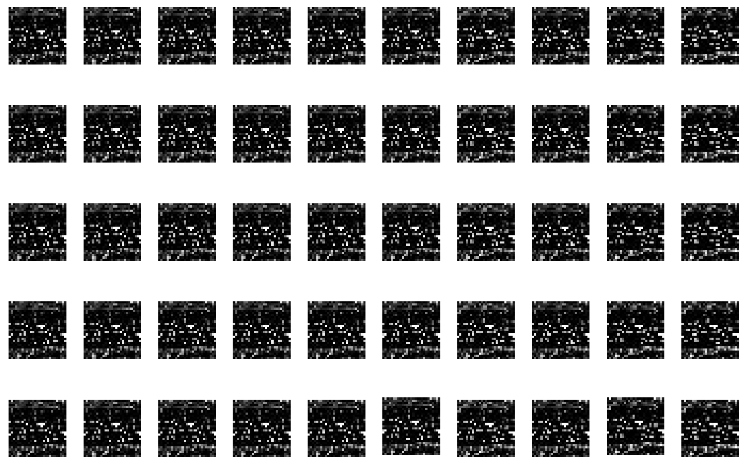
I denotes the normalized indicator function, I = 0 means there is no negative value in the feature column, on the contrary, I = 1 . After the normalization, the normalized value is input into the Formula (3) to generate z × z of the gray-level image matrix. The gray-level image matrix is further converted into an image with a size of z × z , as shown in Figure 2.
During the conversion, When z 2 > d , Corner-Filling is required. Corner-Filling means that when the feature vector is converted into a gray-level image matrix X, it cannot fill X, and it is necessary to supplement the pixel value where it is not filled.
The Corner-Filling is filled with the average value of the feature vector, as shown below.
s u k = 255 j = 1 d a ^ i j d
s u k represents the value that needs to be filled in the u-th row and k-th column of the gray-level image matrix.

The Gray-Level Image Matrix Conversion Algorithm

After the filling is completed, the conversion of the gray-level image can be realized. The detailed flow of the algorithm can be summarized as follows:
In Algorithm 1, the input is the row vector F i a ^ i j R 1 × d of the feature matrix, the feature matrix dimension is d-dimension, and the output is the grayscale image matrix X s i j R z × z , where a ^ i j denotes the j-th element value of F i , j { 1 , 2 , , z } , and  s i j denotes the element value of the i th row and j-th column of X , i , j { 1 , 2 , , z } . Algorithm 1 first calculates the dimension z of the grayscale image matrix based on the dimension d of the feature matrix, and then initializes a z × z grayscale image matrix X. After sufficient preparation, the grayscale value filling starts, which is the value of the elements in the row vector F i passing through the feature matrix. First, a count variable b is defined, and the value b of the count variable is smaller than the feature dimension d. The count variable serves as the index value of F i , i.e.,  a ^ i b denotes the b-th value of F i . Next, the loop traverses the grayscale image matrix X, and fills in the element values of the corresponding feature row vectors, into it. When filling in, if the row vector are completely filled, but the pixels value of X are not completely filled, i.e.,  z 2 > d is filled with missing corners. Finally, the generated grayscale image matrix X is output to complete the grayscale image matrix conversion. The time complexity of the gray-level image matrix conversion Algorithm is O n 2 . The grayscale image conversion is processed only once during data preprocessing, which is relatively within the acceptable time complexity. The algorithm reorganizes the attribute information of features to achieve the processing of interdependent feature information and significantly improves the performance of classification.
Algorithm 1 The Gray-Level Image Matrix Conversion Algorithm
Input: the row vector of Feature Matrix F i a ^ i j R 1 × d , the dimension of Feature Matrix d.
Output: the gray-level image matrix X
1. Calculate the dimensions of the gray-level image matrix z d 2
2. Random init X s i j R z × z
3. Define counting variables b 0
4. for j 1 : z do
5.   for k 1 : z do
6.       if b < d :
7. s j k 255 a ^ i b ;
8. b b + 1 ;
9.       else:
10. s j k 255 p = 1 d a ^ i p d

2.2. Low-Level Feature Extraction Layer

The low-level feature extraction layer is mainly used for low-level feature extraction of images transformed by F2I layer of Section 1 of this Section. The low-level feature extraction layer is integrated with CNN. CNN have always been at the core of significant progress in DL. CNN have a wide range of applications in the field of image processing, including the image classification, target detection, etc. [46,47,48]. Compared with fully connected neural networks, CNN have the advantages of local connection, weight sharing, and downsampling dimensionality reduction [49]. In view of the advantages of CNN, the low-level feature extraction layer is designed according to the architecture of CNN and consists of convolution layer, pooling layer and full connection layer. The low-level feature extraction layer adopts four groups of two-dimensional convolution, one group of one-dimensional convolution, one group of pooling layer and two groups of full connection layer, as shown in Figure 3. The first and second convolution layers adopt 5 × 5 × 64 convolution kernels and use ReLU function as the activation function. The third and fourth convolution layers used 3 × 3 × 32 convolution kernels and ReLU function as the activation function, and the last one used 9 × 9 × 256 convolution kernel and ReLU function as the activation function. The pooling layer selects average pooling to save more background information of image data, and the full connection layer is used for feature fitting.

2.2.1. The Convolution Layer

The convolution layer is mainly used to extract the local features of the feature map generated by the F2I layer. The convolution layer contains multiple convolution kernels, and different convolution kernels extract different local features. The deeper the convolution kernel, the more features of the F2I feature map will be extracted. The local connection and shared parameters between the convolution layers ensure that each convolution kernel can output a local feature.
Let the gray-level image matrix X of the input layer l be δ i l ( i = 1 , 2 , , I ) , the output layer l + 1 feature map is δ j l + 1 ( j = 1 , 2 , , J ) , the input convolution kernel is W j i l + 1 , and the size is K × K . The l + 1 layer feature map of the output can be
δ j 0 = σ w b , δ j 1 = σ i = 1 I w , h K 1 W j i 1 δ i 0 ( x w , y h ) + w b , δ j 2 = σ i = 1 I w , h K 1 W j i 2 ( w , h ) δ i 1 ( x w , y h ) + w b = σ i = 1 I w , h K 1 W j i 2 σ i = 1 I w , h K 1 W j i 1 δ i 0 ( x w , y h ) + w b + w b , , δ j l + 1 ( x , y ) = σ i = 1 I w , h K 1 W j i l + 1 ( w , h ) δ i l ( x w , y h ) + w b
where I represents the depth of the input feature mapping, J represents the depth of the output feature mapping, and  ( x , y ) represents the x-th row and y-th column features of the output feature mapping. ( w , h ) describe the features of row w and column h of the input feature mapping. w b is offset. “*” indicates convolution operation, σ ( · ) represents the activation function. In this paper, R e L U function is selected as the activation function.

2.2.2. The Pooling Layer

The pooling layer is used to reduce the dimension of the feature mapping output from the convolution layer, avoid over fitting and reduce the dimension of the output feature mapping. Pooling treatment is generally divided into maximum pooling and average pooling [50]. Maximum pooling is to use the maximum value in the pooling space, which can effectively extract the texture information of the feature map. Average pooling takes the average value in the pooling space, which can effectively extract the background information of the feature map. According to the characteristics of the two kinds of pooling, this paper adopts average pooling.
To protect the background information of F2I characteristic map to the greatest extent, the calculation method of average pooling is as follows:
f j ( x , y , z ) = 1 x h , 1 y w h , w δ j l + 1 ( x h , y w , z ) h + w = 1 x h , 1 y w h , w σ i = 1 l w , h K 1 W j i l + 1 ( w , h ) δ i l ( x w , y h ) + w b h + w
where ( x , y ) represents the x-th row and y-column features of the output feature map, z represents the eigenvalue, and h and w represent the width and height of the spatial window.

2.2.3. The Full Connection Layer

The function of the full connection layer is to fit the feature mapping output after the multi-layer convolution kernel pooling operation, so as to prepare for the input of the CapsNet module.
Set the input layer l feature mapping to y i l ( i = 1 , 2 , , I ) , the output l + 1 feature map is y j l + 1 ( j = 1 , 2 , , J ) , and the weighted weight is ω j i l + 1 , offset w b . This module is described by:
y i 0 = σ w b y i 1 = σ i = 1 n ω j i 1 y i 0 + w b y i 2 = σ i = 1 n ω j i 2 y i 1 + w b = σ i = 1 n ω j i 2 σ i = 1 n ω j i 1 y i 0 + w b + w b , , y j l + 1 = σ i = 1 n ω j i l + 1 y i l + w b
Among them, σ ( · ) represents the activation function, and n represents the number of neurons. In this paper, R e L U function is selected as the activation function.

2.3. High-Level Feature Extraction Layer

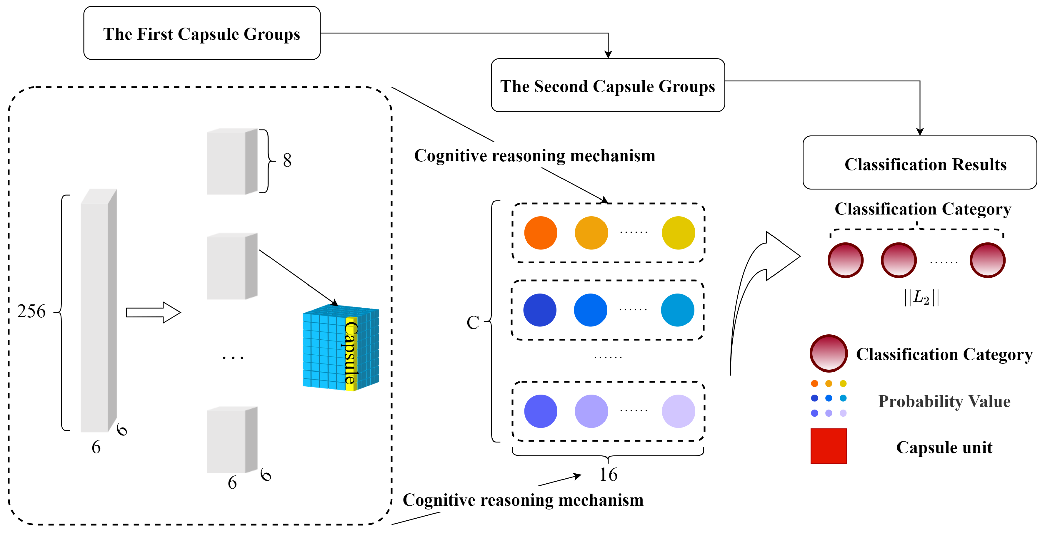
 Based on the low-level extraction layer of Section 2.2 of this Section, The high-level feature extraction layer is used for further extraction of image features, feature combination, cognitive reasoning of features, and category prediction of ADMET properties. The feature mapping extracted by the low-level extraction layer is used as the low-level capsule for this subsection. A capsule is a set of neurons—a vector. The module length of the capsule represents the probability of predicting the class, and the direction represents the instantiation parameter. The capsules of the next layer can predict the capsules of the next layer through cognitive reasoning mechanism. When multiple capsules of the lower layer make the same prediction to the capsules of the upper layer, the capsules of the upper layer will be activated and become the activation vector. The high-level feature extraction layer consists of two groups of capsule layers, as shown in Figure 4. The first group of capsules is composed of 32 6 × 6 × 8 capsules, and the second group of capsules is calculated by cognitive reasoning mechanism. The second group of capsules is composed of C 16- d i m e n s i o n a l digital capsules. Finally, the corresponding probabilities of C categories are output by extrusion function to complete category prediction. See Section 3 for details of the principles and algorithms.

3. Caps3MC Cognitive Reasoning Mechanism and Algorithm

 The cognitive reasoning mechanism is mainly used to perform cognitive reasoning on the features in the high-level feature extraction layer in Section 2. This section focuses on the principle of cognitive reasoning mechanism and the description of related algorithms. The derivation process of cognitive reasoning mechanism is described in Section 3.1 of this Section. Section 3.2 describes the Caps3MC cognitive reasoning algorithm. In Section 3.3 and Section 3.4 of this Section, the derivation process of the loss function and the training process algorithm of the Caps3MC model based on the cognitive reasoning mechanism are described.

3.1. The Cognitive Reasoning Mechanism

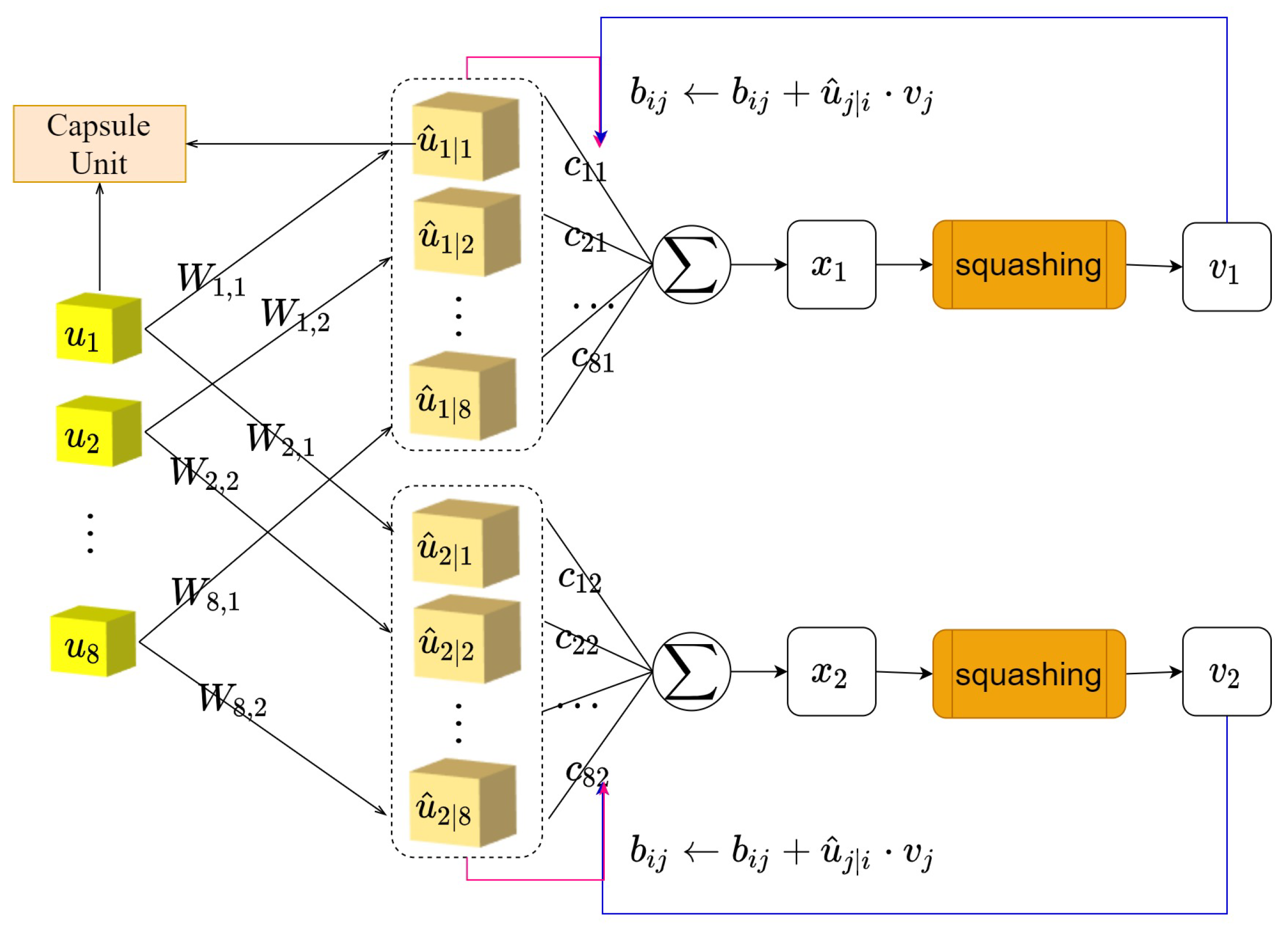
The core of the high-level feature extraction layer is the cognitive reasoning mechanism. The cognitive reasoning mechanism realizes the low-level capsule through the voting mechanism and finds out the relationship between high-level features and low-level features by activating the high-level capsule, as shown in Figure 5.
High-level features and low-level features by activating the high-level capsule. The input of the cognitive reasoning mechanism is 32-th low-level capsule of 6 × 6 × 8 , the number of iterations r and the number of capsule layers l, using u i represents a capsule unit of the lower capsule of the l-th layer. The output is the probability of j-th categories. The cognitive reasoning mechanism first initializes the iteration coefficient b, and the initialization value of b is zero. Multiply the l-th lower capsule u by the weight matrix W of 8 × 16 , which is affine transformed to obtain the high-level capsule u ^ with W i j , which represents an element of the weight matrix W using u ^ j i , which represents a unit of the obtained high-level capsule, then u ^ j i = W i j u i . The category probability capsule v j is as follows:
v 1 = squashing i u ^ 1 i = squashing i W i 1 u i v 2 = squashing i exp v 1 u ^ 1 i exp v 1 u ^ 1 i u ^ 2 i = squashing i exp v 1 W i 1 u i exp v 1 W i 1 u i W i 2 u i , v 3 = squashing i exp v 1 u ^ 1 i + v 2 u ^ 2 i exp v 1 u ^ 1 i + exp v 1 u ^ 1 i + v 2 u ^ 2 i u ^ 3 i = squashing i exp v 1 W i 1 u i + v 2 W i 2 u i exp v 1 W i 1 u i + exp v 1 W i 1 u i + v 2 W i 2 u i W i 3 u i , , , v j = squashing i exp o = 1 j v o u ^ o i exp v 1 u ^ 1 i + exp v 1 u ^ 1 i + v 2 u ^ 2 i + + exp o = 1 j v o u ^ o i u ^ j i = squashing i exp o = 1 j v o W i o u i exp v 1 W i 1 u i + exp v 1 W i 1 u i + v 2 W i 2 u i + + exp o = 1 j v o W i o u i W i j u i
Squashing refers to the squeezing function that compresses the capsule into a probability between [ 0 , 1 ] .
Assume as follows:
b i 1 = v 1 u ^ 1 i , b i 2 = v 1 u ^ 1 i + v 2 u ^ 2 i , , b i j = o = 1 j v o W i o u i = v 1 u ^ 1 i + v 2 u ^ 2 i + v j u ^ j i
We can get this by bringing Formula (8) into Formula (7):
v j = squashing exp b i j k exp b i k u ^ j i
Let the coupling coefficient be c i j = exp b i j k exp b i k , then the digital capsule
x j = i c i j u ^ j i
Then
v j = squashing x j = x j 2 1 + x j 2 x j x j

3.2. Caps3MC Cognitive Reasoning Mechanism Algorithm

 Based on the derivation process of the cognitive reasoning mechanism in the Section 3.1 of this Section, this paper proposes an algorithmic description of the cognitive reasoning mechanism applicable to Caps3MC feature reasoning. The algorithm is described as follows.
The cognitive reasoning mechanism will get the high-level capsule u ^ through the coupling coefficient c i j votes on it and gets j-th 16 dimensional digital capsules x j . The digital capsule x j is compressed into a category probability capsule v j between [ 0 , 1 ] using the squashing function. We update the iteration coefficient b i j until the number of iterations r is reached, where b i j = b i j + u ^ j i v j . Finally, the probability values of each category are compared to predict the category. The cognitive reasoning mechanism iterative process algorithm of Caps3MC model is shown as follows Algorithm 2:
Algorithm 2 The cognitive reasoning mechanism iterative process algorithm
Input: low-level capsule u, Number of iterations r, Number of capsule layers l, Label of the current category j
Output: j-th probability capsule of category v j
1. for all low-level capsule u in layer l and all high-level capsule u ^ in layer ( l + 1 ) : b i j 0 ;
2. for i 1 , 2 , l e n ( u ) do
3. u ^ j i W i j u i , x j i c i j u ^ j i , r 3 ;
4.       for r iterations do
5. c i j exp b i j k exp b i k
6. x j i c i j u ^ j i
7. v j squash x j
8. b i j b i j + u ^ j i v j
9.Return v j
 The algorithm achieves cognitive reasoning from low-level to high-level capsules through a cognitive reasoning mechanism. The complexity of the algorithm is O ( n ) , and the time complexity is calculated mainly from the transformation process of low-level capsules and high-level capsules. The algorithm achieves feature inference through a cognitive reasoning mechanism, which calculates a probabilistic likelihood for each feature, making the final classification results cognitive and interpretable, and significantly improving the classification performance.

3.3. Caps3MC Model Training Loss Function

This section describes the derivation process of the training loss functions for the Caps3MC model based on cognitive reasoning mechanism and algorithm of the Section 3.2 of this Section.
The loss function of Caps3MC model adopts the margin loss function, which limits the upper bound of the edge to m + , and the lower bound of the edge to m .
It is assumed that the probability sample obtained by Caps3MC model is
v 1 , v 2 , , v j , , v n , v j R c , j = 1 , 2 , , n ,
where v j is the probability capsule of c-Dimension, c is the number of categories, and n is the number of samples. These probability samples are linearly separable in R-Dimensional Space, that is, there is a hyperplane
g ( x ) = x 1 2 + x 2 2 + + x c 2 = m 2
So that all probability samples can be separated without error. Where x i R c is the probability capsule v j in the dimensional space, as well as the probability value of predicting a certain category, and m represents the boundary.
If the category predicted by the probability sample exists, the predicted probability sample values are greater than or equal to m + . If the category predicted by the probability sample does not exist, the predicted probability sample values are less than or equal to m . Then, the decision function is
x 1 2 + x 2 2 + + x c 2 m + , x i R c x 1 2 + x 2 2 + + x c 2 m , x i R c
m +  is the edge upper bound, m is the edge lower bound, and c refers to the category of prediction probability. According to Minimum Squared Error criterion, Minimum Squared Error loss from the probability sample to the edge is m | g ( x ) | 2 2 .
For the lower bound of the edge, the loss predicted by the probability sample is
j min 0 , m | g ( x ) | 2 2 s . t . x 1 2 + x 2 2 + + x c 2 2 m 0 , x i R c
Equivalent to
j max 0 , | g ( x ) | 2 m 2 s . t . x 1 2 + x 2 2 + + x c 2 2 m 0 , x i R c
For the edge upper bound, the loss of the probability sample is
j min 0 , | g ( x ) | 2 m + 2 s . t . x 1 2 + x 2 2 + + x c 2 2 m + 0 , x i R c
Equivalent to
j max 0 , m + | g ( x ) | 2 2 s . t . x 1 2 + x 2 2 + + x c 2 2 m + 0 , x i R c
For all probability samples, there are only two kinds of predicted categories: categories that exist and categories that do not exist, that is, category samples are mutually exclusive. If I is defined as the classification indicator function, I = 1 when the predicted category exists and I = 0 when the predicted category does not exist. Then the loss of all probability samples is
j I j max 0 , m + v j 2 + 1 I j max 0 , v j m 2
In the process of model training, the proportion of category samples will be unbalanced. Therefore, a weight factor is added to adjust the proportion of category existence and non-existence. The final loss function is
Caps3MC_Loss = j I j max 0 , m + v j 2 + 1 I j max 0 , v j m 2
where m + represents the upper bound of the edge and m represents the lower bound of the edge. v j is the probability capsule, indicating the probability that the output belongs to a certain category, v j represents the L 2 norm of a capsule. λ is a weight factor. In order to reduce when a certain type does not appear, all activated digital capsules are compressed. In this paper λ = 0.5 , m + = 0.9 , m = 0.1 .

3.4. Caps3MC Model Training Progress Algorithm

This subsection describes the training process algorithm for the Caps3MC model based on the algorithm description of the cognitive reasoning mechanism in Section 3.2 of this Section and the loss function in Section 3.3 of this Section.
In the learning process, the model first converts the data set into graph data through the F2I conversion model, and segments the data set according to the proportion that the training set accounts for 70% of the total sample and the test set accounts for 30% of the total sample. We input the segmented data set to the low-level feature extraction layer, and the output of the low-level feature extraction layer is the input of the high-level feature extraction layer. The high-level feature extraction layer outputs the possible probability of each category, and selects the one with high probability as the prediction category of the category by comparing the probability, so as to realize category prediction.This paper briefly describes the training process of the proposed Caps3MC model, and the progress is described as follows Algorithm 3:
Algorithm 3 The training process of the Caps3MC model
Input: Dataset with n rows and d columns, training epochs T.
Output: Category of prediction.
1. Initialize grayscale image data set X ^ ;
2. for row 1 , 2 , , n do
3.   Select the r row of the data set and convert it into gray image matrix X through F2I model;
4.   Add X to X ^ ;
5. Will X ^ The training set and test set are exchanged according to 7:3;
6. for Epoch = 1 , 2 , , T do
7.    Training Caps3MC model with training set;
8.    Using C a p s 3 M C _ L o s s calculation model training loss update model parameters;
9.    Validate the model using a test set;
10. Compare the probability of each category and output the prediction results.

4. Experimental Analysis

In this section, Intestinal epithelial cell permeability (Caco-2), cytochrome P450 (CYP) 3A4 subtype (CYP3A4), human ether-a-go-go related gene (hERG), human oral bioavailability (HOB) and micronucleus test were used (micronucleus, MN) five ADMET properties are used to experimentally verify the model Caps3MC. The specific ADMET property information is listed in Table 1. In order to better show the performance of Caps3MC model, this paper compares the experimental results of Caps3MC model with decision tree classification model, support vector machine classification model, logistic regression classification model, k-nearest neighbor classification model, Bayesian classification model, and Fisher linear discrimination model The classification model is analyzed, and the experimental results of six ML models and CNN model are compared and analyzed. This section may be divided by subheadings. It should provide a concise and precise description of the experimental results, their interpretation, and the experimental conclusions that can be drawn.

4.1. Data set

In this section, we used the bioactive data of compounds targeting breast cancer treatment targets Er α to achieve intestinal permeability (Caco-2), Cytochrome P450 (CYP) 3A4 subtype (CYP3A4), and compound cardiac safety assessment (human Ether-a-go-go Related Gene, P450). Human oral bioavailability (HOB) and micronucleus test (MN) are five categories of ADMET properties. The meanings represented by each category label are listed in Table 2.
In this paper, the data set is divided into a training set and a test set using the cross validation method. The training set is used to train the model, and the test set is used to test and verify the model.

4.2. Experimental Evaluation Index

In medicine, Positive and Negative are usually used for dichotomous problems that stand for two categories. Positive means that a symptom exists and negative means that a symptom does not exist. Disease diagnosis is a dichotomous problem of positive and negative judgment. There are only two possible positive or negative categories for a sample. Therefore, there are four decision results: True Positive ( T P ) , False Positive ( F P ) , True Negative ( T N ) , and False Negative ( F N ) .
Calculate the P r e c i s i o n rate, R e c a l l rate, and the F 1 value of model classification according to the decision results.
P r e c i s i o n rate: Among all the samples predicted as positive examples, the proportion of samples as positive examples is defined as
P r e c i s i o n = T P T P + F P
R e c a l l rate: Among all the samples that are actually positive examples, the proportion predicted as positive examples is defined as
R e c a l l = T P T P + F N
F 1 value: The P r e c i s i o n rate and R e c a l l rate are a pair of contradictory measures. Generally speaking, when the P r e c i s i o n rate is high, the R e c a l l rate is often low, while when the R e c a l l rate is high, the P r e c i s i o n rate is often low. Therefore, F 1 harmonic mean value is adopted, which is defined as
F 1 = 1 1 2 1 P r e c i s i o n + 1 R e c a l l = 2 T P + F P T P + T P + F N T P = 2 T P 2 T P + F P + F N
In addition to the above indicators, the Area Under Curve(AUC) value is used as the indicator of the measurement model. The AUC value is the area below the receiver operating characteristic curve(ROC). The AUC value is usually between (0.5, 1]. The larger the value, the better the model is.

4.3. Analysis of Experimental Results

In this section, the analysis of experimental results is divided into two parts: the first part is the analysis of the performance results of Caps3MC model for the classification of five ADMET properties; The second part is the comparative experimental results of Caps3MC model with other six ML classification models and CNN model. When using CNN model for training, for the sake of fairness, CNN adopts the same parameters as Caps3MC for training.

4.3.1. Analysis of Experimental Results of Caps3MC Model

The number of iterations of epochs used in the training model is 1000, and 5 categories are trained, respectively. The training process is shown in Figure 6.
The P r e c i s i o n rate, R e c a l l rate, F 1 value, and AUC value are calculated according to the number of four decision results. In order to make the evaluation indexes of the experimental data more referential, this experiment weighted the average P r e c i s i o n rate, R e c a l l rate, and F 1 value, and calculated the cumulative sum of the proportion of a certain category of samples in the overall sample and the product of the corresponding P r e c i s i o n rate, R e c a l l rate, and F 1 value to obtain the weighted P r e c i s i o n rate, weighted R e c a l l rate, and the weighted F 1 value. The experimental evaluation results are listed in Table 3.
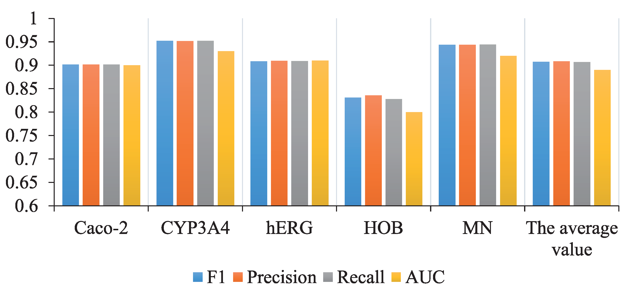
From the analysis of the data presented in Table 3 and Figure 7, the weighted P r e c i s i o n rate, weighted R e c a l l rate, and weighted F 1 value predicted by Caps3MC model for Caco-2, CY P3A4, HERG, HOB and MN are more than 90%. Among them, Caps3MC has the highest accuracy of CYP3A4 prediction, reaching 95.16%. The AUC predicted by Caps3MC model for five ADMET property categories is up to 0.93, and the average value is close to 0.90.

4.3.2. Analysis of Comparative Experimental Results

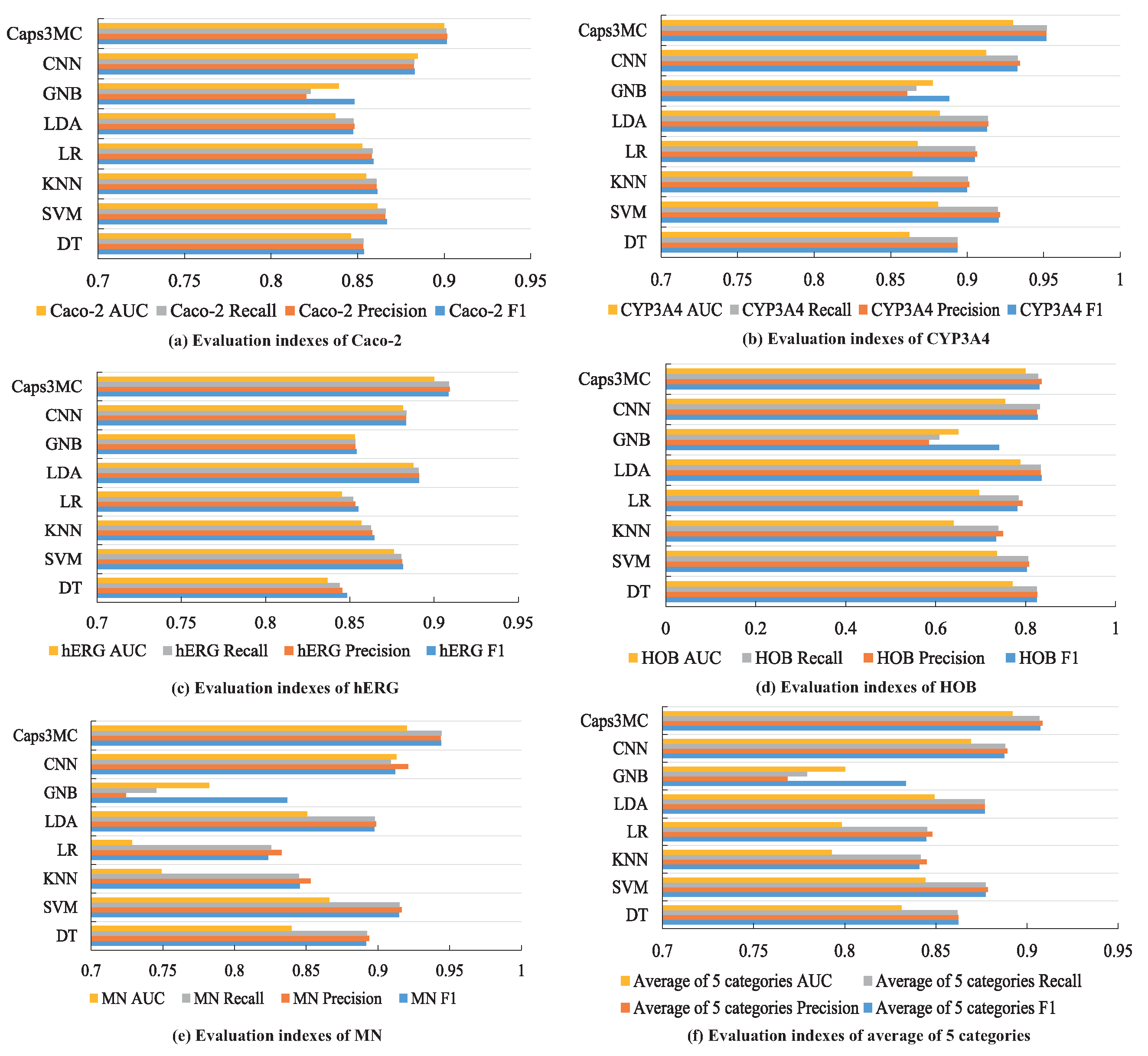
In order to demonstrate the performance of the model, six ML classification models and CNN model are selected for comparison. The ML model includes the DT, SVM, KNN, LR, LDA, and GNB classification model. Comparison experimental results are listed in Table 4,bold results in the table are the best results. According to the data analysis in Table 4 and Figure 8, among the predicted evaluation indexes of Caco-2, weighted P r e c i s i o n rate, weighted R e c a l l rate, weighted F 1 value, and AUC value corresponding to the other six ML classification models and the CNN model are the highest. Compared with the evaluation results of Caps3MC model, it can be observed that the four evaluation indexes of the model are about 4 % higher than those of the other six ML classification models and about 2 % of the CNN model. The three evaluation indexes of the corresponding ML classification model for CYP3A4 prediction are higher than about 3 % , and the AUC value is higher than about 5 % . Four indexes of the DL model are higher than about 2 % . The corresponding four evaluation indexes of the ML classification model predicted by HERG are higher than about 1 % . Four evaluation indexes of CNN model are higher than about 2 % . Three evaluation indexes of the corresponding ML classification model for HOB prediction are higher than about 1 % , and the R e c a l l rate of Caps3MC model is lower than that of the LDA classification model by about 1 % ; The three indexes of the DL model are higher than about 1 % , and the R e c a l l rate of Caps3MC model is lower than that of the CNN model by about 1 % . The three indexes of the ML classification model predicted by MN are higher than about 3 % , and the AUC value is higher than about 6 % ; The three evaluation indexes of CNN model are higher than about 2 % , and the AUC value is higher than about 1 % .
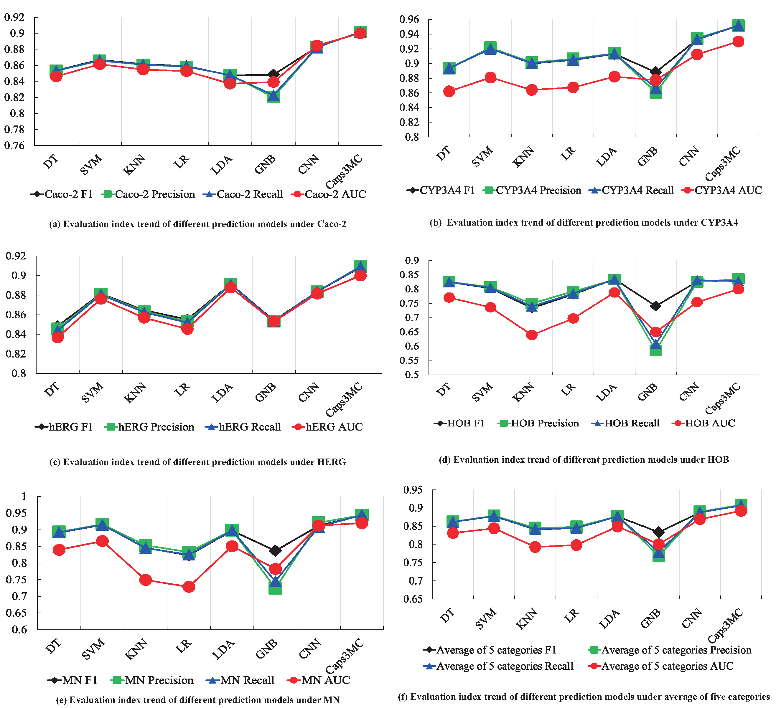
Figure 9 clearly shows the evaluation index results and trends of the average values of Caco-2, CYP3A4, hERG, HOB, MN, and average of five categories under Caps3MC, four evaluation indexes of six machine learning models and CNN deep learning model. Different color curves represent different evaluation indexes.
As can be seen from the evaluation index trends of different classification models in Figure 9 compared with the evaluation index trends under five ADMET properties, the prediction results of the Caps3MC model are more accurate and very close to the real data classification. Comparing the evaluation trend under the average value of five categories, the evaluation effect of Caps3MC model is much higher than that of the other seven models, and has better comprehensive classification performance and classification accuracy.
Through comparison and comprehensive consideration of the comparison between Caps3MC model and six classification models and CNN model, it can be possible to conclude that the Caps3MC model has significant advantages.

5. Conclusions

In this paper, Caps3MC model is proposed to better predict the ADMET properties of compounds. The model consists of three parts. Firstly, the Caps3MC model uses the F2I module to convert the feature vector of each instance in the structured data into a gray image matrix, which is input into low-level feature extraction layer after matrix transformation. Secondly, the Caps3MC model uses the gray image generated by low-level feature extraction layer to realize the preliminary feature extraction. After being processed by the low-level feature extraction layer, the output feature mapping is used as the input of the high-level feature extraction layer. Finally, the Caps3MC model uses high-level feature extraction layer to further extract the features from the feature map output by low-level feature extraction layer. We use the cognitive reasoning mechanism to realize low-level capsule and activate high-level capsule, so as to further quantify and extract the feature correlation. Finally, the active high-level capsule is compressed into a probability capsule between [0, 1] through the extrusion function, the probability of each category is compared, the prediction category is output, and finally the category prediction is realized. Compared with DT, SVM, KNN, LR, LDA, NB and CNN model, the Caps3MC model has higher accuracy and significant classification performance.
At the same time, this study has some defects. Firstly, when facing the data set with a small amount of feature data, the F2I conversion module converts it into a very small picture, which greatly reduces the classification effect of the model, but on the contrary, the data set with a large number of features will show excellent performance and effect. In the future, we will consider solving this problem by combining the algorithm or introducing the feature scaling algorithm. Secondly, in the case of corner missing filling, the problem of “feature disappearance” will occur when the corner missing is serious, but in most cases, there is no serious corner missing. In the future, attention mechanism will be introduced to eliminate the problem of “feature disappearance”, so as to make the robustness of the model stronger.
Finally, in the field of medicine, there are a large number of multimodal data in candidate drug prediction, not only pure index data, but also text, image and other data, which brings challenges to the research and will be the key direction of drug prediction in the future.

Author Contributions

Conceptualization, J.W.; methodology, J.W.; formal analysis, J.W.; writing—review and editing, J.W.; writing—original draft preparation, D.Z.; software, D.Z.; validation, D.Z.; investigation, L.L.; resources, L.L.; data curation, L.L. All authors have read and agreed to the published version of the manuscript.

Funding

This research was supported by Hebei Natural Science Foundation (F2021205014),funded by Science and Technology Project of Hebei Education Department (ZD2022139), supported by the Natural Science Foundation of Hebei Province (F2019205303), funded by The Introduction of Overseas Students in Hebei Province (C20200340), supported by the Hebei Normal University Science and Technology Fund Project (L2019Z10).

Institutional Review Board Statement

Not applicable.

Informed Consent Statement

Not applicable.

Data Availability Statement

Not applicable.

Conflicts of Interest

The authors declare no conflict of interest.

References

  1. Mohammad, R. Design, synthesis and ADMET prediction of bis-benzimidazole as anticancer agent. Bioorganic Chem. 2020, 96, 103576. [Google Scholar] [CrossRef]
  2. Feinberg, E.N.; Joshi, E.; Pande, V.S.; Cheng, A.C. Improvement in ADMET prediction with multitask deep featurization. J. Med. Chem. 2020, 63, 8835–8848. [Google Scholar] [CrossRef]
  3. Hiba, A.; Hajar, M.; Hassan, A.; Thomas, N. Design, Using Machine Learning Algorithms for Breast Cancer Risk Prediction and Diagnosis. Procedia Comput. Sci. 2016, 83, 1064–1069. [Google Scholar] [CrossRef] [Green Version]
  4. Yin, S.; Xi, R.; Wu, A.; Wang, S.; Li, Y.; Wang, C.; Tang, L.; Xia, Y.; Yang, D.; Li, J.; et al. Design, Patient-derived tumor-like cell clusters for drug testing in cancer therapy. Sci. Transl. Med. 2020, 12, 549. Available online: https://www.science.org/doi/10.1126/scitranslmed.aaz1723 (accessed on 12 April 2022). [CrossRef]
  5. Chen, Z.; Cao, Y.; He, S.; Qiao, Y. Development of models for classification of action between heat-clearing herbs and blood-activating stasis-resolving herbs based on theory of traditional Chinese medicine. Chin. Med. 2018, 13, 12. [Google Scholar] [CrossRef] [Green Version]
  6. Lu, W.; Li, Z.; He, S.; Chu, J. A novel computer-aided diagnosis system for breast MRI based on feature selection and ensemble learning. Comput. Biol. Med. 2017, 83, 157–165. [Google Scholar] [CrossRef] [PubMed]
  7. Aslan, M.F.; Celik, Y.; Sabanci, K.; Durdu, A. Breast cancer diagnosis by different machine learning methods using blood analysis data. Int. J. Intell. Syst. Appl. Eng. 2018, 6, 289–293. [Google Scholar] [CrossRef]
  8. Nindrea, R.D.; Aryandono, T.; Lazuardi, L.; Dwiprahasto, D. Diagnostic Accuracy of Different Machine Learning Algorithms for Breast Cancer Risk Calculation: A Meta-Analysis. Asian Pac. J. Cancer Prev. APJCP 2018, 19, 1747. [Google Scholar] [CrossRef]
  9. Fagerholm, U.; Hellberg, S.; Spjuth, O. Advances in Predictions of Oral Bioavailability of Candidate Drugs in Man with New Machine Learning Methodology. Molecules 2021, 26, 2572. [Google Scholar] [CrossRef]
  10. Onay, A.; Onay, M. A drug decision support system for developing a successful drug candidate using machine learning technique. Curr. Comput. Aided Drug Des. 2020, 16, 407–419. [Google Scholar] [CrossRef]
  11. Yuan, K.H.; Xu, W.H.; Li, W.T.; Ding, W.P. An incremental learning mechanism for object classificationbased on progressive fuzzy three-way concept. Inf. Sci. 2022, 584, 127–147. [Google Scholar] [CrossRef]
  12. Chen, X.W.; Xu, W.H. Doublequantitative multigranulation rough fuzzy set based on logical operations in multisource decision systems. Int. J. Mach. Learn. Cybern. 2021, 13, 1021–1048. [Google Scholar] [CrossRef]
  13. Li, W.T.; Xu, W.H.; Zhang, X.Y.; Zhang, J. Updating approximations with dynamic objects based on local multigranulation rough sets in ordered information systems. Artif. Intell. Rev. 2021, 55, 1821–1855. [Google Scholar] [CrossRef]
  14. Ferreira, L.L.G.; Andricopulo, A.D. ADMET modeling approaches in drug discovery. Drug Discov. Today 2019, 24, 1157–1165. [Google Scholar] [CrossRef] [PubMed]
  15. Sasahara, K.; Shibata, M.; Sasabe, H.; Suzuki, T.; Takeuchi, K.; Umehara, K.; Kashiyama, E. Feature importance of machine learning prediction models shows structurally active part and important physicochemical features in drug design. Drug Metab. Pharmacokinet. 2021, 39, 100401. [Google Scholar] [CrossRef] [PubMed]
  16. Schneider, P.; Walters, W.; Plowright, A.T.; Sieroka, N.; Listgarten, J.; Goodnow, R.A., Jr.; Jansen, J.M.; Duca, J.S.; Rush, T.S.; Zentgraf, M.; et al. Rethinking drug design in the artificial intelligence era. Nat. Rev. Drug Discov. 2020, 19, 353–364. [Google Scholar] [CrossRef] [PubMed]
  17. Kumar, K.; Chupakhin, V.; He, S.; Vos, A.; Morrison, D.; Rassokhin, D.; Dellwo, M.J.; McCormick, K.; Paternoster, E.; Ceulemans, H.; et al. Development and implementation of an enterprise-wide predictive model for early absorption, distribution, metabolism and excretion properties. Future Med. Chem. 2021, 13, 1639–1654. [Google Scholar] [CrossRef]
  18. Jiang, D.; Lei, T.; Wang, Z.; Shen, C.; Cao, D.; Hu, T. ADMET evaluation in drug discovery. 20. Prediction of breast cancer resistance protein inhibition through machine learning. J. Cheminformatics 2020, 12, 16. [Google Scholar] [CrossRef] [Green Version]
  19. De Moura, É.P.; Fernandes, N.D.; Monteiro, A.F.M.; De Medeiros, H.R.; Tullius, S.M.; Luciana, S. Machine Learning, Molecular Modeling, and QSAR Studies on Natural Products Against Alzheimer’s Disease. Curr. Med. Chem. 2021, 38, 7808–7829. [Google Scholar] [CrossRef]
  20. Bannigan, P.; Aldeghi, M.; Bao, Z.; Florian Hse, F.; Aspuru-Guzik, A.; Allen, C. Machine learning directed drug formulation development. Adv. Drug Deliv. Rev. 2021, 175, 113806. [Google Scholar] [CrossRef]
  21. Jaganathan, K.; Tayara, H.; Chong, K.T. An Explainable Supervised Machine Learning Model for Predicting Respiratory Toxicity of Chemicals Using Optimal Molecular Descriptors. Pharmaceutics 2020, 14, 832. [Google Scholar] [CrossRef] [PubMed]
  22. Ekins, S.; Puhl, A.C.; Zorn, K.M.; Lane, T.R.; Russo, D.P.; Klein, J.J.; Clark, A.M. Exploiting machine learning for end-to-end drug discovery and development. Nat. Mater. 2019, 18, 435–441. [Google Scholar] [CrossRef] [PubMed]
  23. Shou, W.Z. Current status and future directions of high-throughput ADME screening in drug discovery. J. Pharm. Anal. 2020, 10, 201–208. [Google Scholar] [CrossRef] [PubMed]
  24. Vatansever, S.; Schlessinger, A.; Wacker, D.; Kaniskan, H.; Jin, J.; Zhou, M.M.; Zhang, B. Artificial intelligence and machine learningaided drug discovery in central nervous system diseases: Stateofthearts and future directions. Med. Res. Rev. 2021, 41, 1427–1473. [Google Scholar] [CrossRef] [PubMed]
  25. Ai, H.; Wu, X.; Zhang, L.; Qi, M.; Zhao, Y.; Zhao, Q.; Liu, H. QSAR modelling study of the bioconcentration factor and toxicity of organic compounds to aquatic organisms using machine learning and ensemble methods. Nat. Mater. 2019, 179, 71–78. [Google Scholar] [CrossRef]
  26. Nayarisseri, A.; Khandelwal, R.; Tanwar, P.; Madhavi, M.; Sharma, D.; Thakur, G.; Singh, S.K. Artificial intelligence, big data and machine learning approaches in precision medicine & drug discovery. Curr. Drug Targets 2019, 22, 631–655. [Google Scholar] [CrossRef]
  27. Jia, C.Y.; Li, J.Y.; Hao, G.F.; Yang, G.F. A drug-likeness toolbox facilitates ADMET study in drug discovery. Drug Discov. Today 2020, 25, 248–258. [Google Scholar] [CrossRef]
  28. Xu, W.H.; Yuan, K.H.; Li, W.T. Dynamic updating approximations of local generalized multigranulation neighborhood rough set. Appl. Intell. 2022, 16, 1–26. [Google Scholar] [CrossRef]
  29. Xu, W.H.; Yu, J.H. A novel approach to information fusion in multi-source datasets: A granular computing viewpoint. Inf. Sci. 2017, 378, 410–423. [Google Scholar] [CrossRef]
  30. Minnich, A.J.; McLoughlin, K.; Tse, M.; Deng, J.; Weber, A.; Murad, N.; Allen, J.E. AMPL: A data-driven modeling pipeline for drug discovery. J. Chem. Inf. Model. 2020, 60, 1955–1968. [Google Scholar] [CrossRef] [PubMed]
  31. Xu, W.H.; Guo, Y.T. Generalized multigranulation double-quantitative decision-theoretic rough set, Knowledge-Based Systems. Knowl. Based Syst. 2016, 105, 190–205. [Google Scholar] [CrossRef]
  32. Xu, W.H.; Li, W.T. Granular computing approach to two-way learning based on formal concept analysis in fuzzy datasets. IEEE Trans. Cybern. 2016, 46, 366–379. [Google Scholar] [CrossRef] [PubMed]
  33. Kumar, A.; Kini, S.G.; He, S.; Rathi, E. A recent appraisal of artificial intelligence and in silico ADMET prediction in the early stages of drug discovery. Mini Rev. Med. Chem. 2021, 21, 2788–2800. [Google Scholar] [CrossRef] [PubMed]
  34. Wallach, I.; Dzamba, M.; Heifets, A. Atomnet: A deep convolutional neural network for bioactivity prediction in structure-based drug discovery. Math. Z. 2015, 47, 34–46. [Google Scholar]
  35. Chen, H.; Engkvist, O.; Wang, Y.; Olivecrona, M.; Blaschke, T. The rise of deep learning in drug discovery. Drug Discov. Today 2018, 23, 1241–1250. [Google Scholar] [CrossRef]
  36. Kearnes, S.; McCloskey, K.; Berndl, M.; Pande, V.; Riley, P. Molecular graph convolutions: Moving beyond fingerprints. J. Comput. Aided Mol. Des. 2016, 30, 595–608. [Google Scholar] [CrossRef] [Green Version]
  37. Shi, T.; Yang, Y.; Huang, S.; Chen, L.; Kuang, Z.; Heng, Y.; Mei, H. Molecular image-based convolutional neural network for the prediction of ADMET properties. Chemom. Intell. Lab. Syst. 2019, 194, 103853. [Google Scholar] [CrossRef]
  38. Sun, K.; Wen, X.B.; Yuan, L.M.; Xu, H.X. Dense capsule networks with fewer parameters. Soft Comput. 2021, 25, 6927–6945. [Google Scholar] [CrossRef]
  39. Hinton, G.E.; Krizhevsky, A.; Wang, S.D. Transforming Auto-Encoders. In International Conference on Artificial Neural Networks; Springer: Berlin/ Heidelberg, Germany, 2011; Volume 13, pp. 44–51. [Google Scholar] [CrossRef] [Green Version]
  40. Patrick, M.K.; Adekoya, A.F.; Mighty, A.A.; Edward, B.Y. Capsule networksa survey. J. King Saud Univ.-Comput. Inf. Sci. 2022, 34, 1295–1310. [Google Scholar] [CrossRef]
  41. Sabour, S.; Frosst, N.; Hinton, G.E. Dynamic routing between capsules. In Proceedings of the Conference and Workshop on Neural Information Processing Systems, Long Beach, CA, USA, 4–9 December 2017; Available online: https://arxiv.53yu.com/abs/1710.09829 (accessed on 12 April 2022).
  42. Hinton, G.E.; Sabour, S.; Frosst, N. Matrix capsules with EM routing. In Proceedings of the International Conference on Learning Representations, Vancouver Convention Center, Vancouver, BC, Canada, 30 April–3 May 2018; Available online: https://openreview.net/pdf?id=HJWLfGWRb (accessed on 12 April 2022).
  43. Wang, J.H.; Han, D.L.; Chen, Y.Y. Image label noise preprocessing method based on combination domain. J. Nanjing Univ. Sci. Technol. 2021, 45, 558–566. [Google Scholar] [CrossRef]
  44. Wang, J.H.; Liang, L.N.; Hao, K.; Zhou, Y. Community discovery algorithm based on attention network feature. Shandong Daxue Xuebao (Lixue Ban) 2021, 56, 13. [Google Scholar] [CrossRef]
  45. Cai, B.; Wang, Y.; Zeng, L.; Hu, Y.; Li, H. Edge classification based on Convolutional Neural Networks for community detection in complex network. Phys. A Stat. Mech. Appl. 2020, 556, 124826. [Google Scholar] [CrossRef]
  46. Yu, W.; Sun, X.; Yang, K.; Rui, Y.; Yao, H. Hierarchical semantic image matching using CNN feature pyramid. Comput. Vis. Image Underst. 2018, 169, 40–51. [Google Scholar] [CrossRef]
  47. Yao, X.; Wang, X.; Wang, S.H.; Zhang, Y.D. A comprehensive survey on convolutional neural network in medical image analysis. Multimed. Tools Appl. 2020, 8, 1–45. [Google Scholar] [CrossRef]
  48. Elngar, A.A.; Arafa, M.; Fathy, A.; Moustafa, B.; Mahmoud, O.; Shaban, M.; Fawzy, N. Image Classification Based on CNN: A Survey. J. Cybersecur. Inf. Manag. (JCIM) 2021. [Google Scholar] [CrossRef]
  49. Khan, A.; Sohail, A.; Zahoora, U.; Qureshi, A.S. A survey of the recent architectures of deep convolutional neural networks. Artif. Intell. Rev. 2020, 53, 5455–5516. [Google Scholar] [CrossRef] [Green Version]
  50. Hyun, J.; Seong, H.; Kim, E. Universal pooling—A new pooling method for convolutional neural networks. Expert Syst. Appl. 2021, 180, 115084. [Google Scholar] [CrossRef]
Figure 1. Caps3MC model.
Symmetry 14 01034 g001
Figure 2. A part of the images transformed from the F2I model.
Symmetry 14 01034 g002
Figure 3. The low-level feature extraction layer of the Caps3MC model.
Symmetry 14 01034 g003
Figure 4. The high-level feature extraction layer of Caps3MC.
Symmetry 14 01034 g004
Figure 5. The cognitive reasoning mechanism of the Caps3MC model.
Symmetry 14 01034 g005
Figure 6. Training progress of the Caps3MC model. (a) Training progress of Caco-2. (b) Training progress of CYP3A4. (c) Training progress of hERG. (d) Training progress of HOB. (e) Training progress of MN.
Symmetry 14 01034 g006
Figure 7. Statistics of different evaluation indexes of Caps3MC model under five categories.
Symmetry 14 01034 g007
Figure 8. Statistical evaluation indexes of different models under five categories.
Symmetry 14 01034 g008
Figure 9. The evaluation index values of different classification models are obtained.
Symmetry 14 01034 g009
Table 1. Description of ADMET.
ADMET Property NameADMET Property AbbreviationADMET Property Description
Permeability of small intestinal epithelial cellsCaco-2It can measure the ability of compounds to be absorbed by the human body
Cytochrome P450 enzyme (Cytochrome P450, CYP) 3A4 SubtypeCYP3A4The main metabolic enzymes in the human body can measure the metabolic stability of compounds
Cardiac safety evaluation of compoundshERGCardiotoxicity of measurable compounds
Human oral bioavailabilityHOBIt can measure the proportion of drugs absorbed into the human blood circulation after entering the human body
Micronucleus testMNIs to detect whether the compound has genotoxicity
Table 2. Description of ADMET classification.
ADMET PropertiesLabelLabel Content
Caco-20Indicates that the permeability of small intestinal epithelial cells of the compound is poor
1Indicates that the permeability of small intestinal epithelial cells of the compound is good
CYP3A40Indicates that the compound cannot be metabolized by CYP3A4
1Indicates that the compound can be metabolized by CYP3A4
hERG0Indicates that the compound has no cardiotoxicity
1Indicates that the compound has cardiotoxicity
HOB0Indicates that the oral bioavailability of the compound is poor
1Indicates that the oral bioavailability of the compound is good
MN0Indicates that the compound is not genotoxic
1Indicates that the compound is genotoxic
Table 3. Description of ADMET classification.
ADMET PropertiesF 1 PrecisionRecallAUC
Caco-290.14%90.17%90.13%0.9
CYP3A495.17%95.16%95.19%0.93
hERG90.85%90.94%90.89%0.91
HOB83.08%83.55%82.78%0.8
MN94.39%94.37%94.43%0.92
Average 190.73%90.84%90.68%0.89
1 The last row of the table represents the average value of the five ADMET property evaluation indicators.
Table 4. Omparative experimental evaluation results of seven algorithms for the Caps3MC model.
DatasetEvaluation IndexDTSVMKNNLRLDAGNBCNNCaps3MC
Caco-2F185.36%86.69%86.14%85.91%84.75%84.82%88.29%90.14%
Precision85.32%86.58%86.08%85.82%84.81%82.03%88.24%90.17%
Recall85.33%86.62%86.10%85.86%84.77%82.27%88.27%90.13%
AUC0.84620.86140.85480.85270.83710.83910.88480.9
CYP3A4F189.37%92.04%90.00%90.49%91.30%88.82%93.26%95.17%
Precision89.37%92.15%90.13%90.63%91.39%86.08%93.44%95.16%
Recall89.37%92.00%90.05%90.52%91.34%86.67%93.29%95.19%
AUC0.86210.88090.86410.86750.88210.87750.91240.93
hERGF184.84%88.15%86.45%85.52%89.12%85.40%88.35%90.85%
Precision84.56%88.10%86.33%85.32%89.11%85.32%88.35%90.94%
Recall84.40%88.05%86.24%85.19%89.09%85.34%88.36%90.89%
AUC0.83680.87620.85680.84540.88770.8530.88150.9
HOBF182.48%80.31%73.39%78.15%83.52%74.05%82.64%83.08%
Precision82.53%80.76%74.94%79.24%83.29%58.48%82.48%83.55%
Recall82.50%80.50%73.93%78.45%83.39%60.82%83.13%82.78%
AUC0.77040.73610.63930.69710.78830.64980.75420.8
MNF189.17%91.47%84.56%82.35%89.74%83.68%91.20%94.39%
Precision89.37%91.65%85.32%83.29%89.87%72.41%92.11%94.37%
Recall89.24%91.49%84.49%82.54%89.79%74.53%90.89%94.43%
AUC0.83990.86610.74910.72840.85070.78230.91280.92
Average of Five CategoriesF186.24%87.73%84.10%84.48%87.68%83.35%88.75%90.73%
Precision86.23%87.85%84.50%84.80%87.69%76.86%88.92%90.84%
Recall86.17%87.73%84.16%84.51%87.67%77.92%88.79%90.68%
AUC0.83110.84410.79280.79820.84910.80030.869140.892
Publisher’s Note: MDPI stays neutral with regard to jurisdictional claims in published maps and institutional affiliations.