Comprehensive Geographic Networks Analysis: Statistical, Geometric and Algebraic Perspectives

Abstract

Using complex network analysis methods to analyze the internal structure of geographic networks is a popular topic in urban geography research. Statistical analysis occupies a dominant position in the current research on geographic networks. This perspective mainly focuses on node connectivity, while other perspectives, such as geometric and algebraic perspectives, can provide additional insights into network structure. Using 11 different real-world geographic networks as examples, this study examines geographic networks from statistical, geometric, and algebraic perspectives. The following are some of the paper’s new findings: (1) When viewed statistically, geometrically, and algebraically, geographic networks have completely different properties. The statistical perspective describes both local and global connectivity; the Ricci curvature in the geometric perspective can assess the network’s development potential as well as describe its transmission capability, and the algebraic perspective can capture the global network topology other than connectivity; (2) Networks are qualitatively and quantitatively classified from three perspectives. The classification results are in accordance with the topological robustness experiment results, which indicate that an analysis from many angles has a lot of practical relevance; (3) Statistical indicators are better than Ricci curvature in identifying essential nodes in networks from a geometric standpoint, whereas the latter is better at detecting significant edges. Overall, studying geographic networks from various perspectives may provide new insights into their understanding.

1. Introduction

When studying the relationships between elements in a system, researchers often use the form of a network to model the system, i.e., the elements are abstracted as nodes, and the relationships between elements are abstracted as edges, with an attempt to obtain knowledge by analyzing the network. Geographic systems are no exception. In geographic research, transportation systems, as typical complex spatial networks, have received strong attention in the field of complex network research [1,2,3]. In addition to transportation systems, global trade activities [4], urban spatial divisions [5], industrial clusters [6], temperature data [7] and even climate hydrological factors [8,9] can be studied abstractly as networks.

The objective of modeling a geographic system as a complex network is to grasp the underlying nature of geographically complex phenomena and processes. The key to achieving this is to examine the geographic network structure. When studying the structural characteristics of complex networks, many models and indicators have been proposed to characterize the structural characteristics of networks. These methods can be classified into three types of perspectives. Due to the different mathematical theories behind them, the three perspectives can characterize the network with different focuses. The statistical perspective is derived from statistical physics, which focuses on the connectivity properties of the nodes in the network. The geometric perspective originates from differential geometry, and it focuses on the transmission properties of the edges in the network. The spectral perspective originates from matrix analysis and focuses on the global structural information of the network.

The statistical perspective is the mainstream perspective currently used for complex network analysis. Indicators based on this perspective mainly describe the topological connection characteristics based on the statistical characteristics of nodes or edges, such as the degree, average path length, clustering coefficient, and betweenness centrality. Some most representative complex network models [10,11,12] are also characterized by these statistical indicators. Indicators from a statistical perspective can also become scalable to investigate the properties of large-scale nodes and their connections in the network. However, existing research has discovered that statistically similar networks can exhibit radically different behaviors when viewed from different perspectives [13]. Thus, it is insufficient to characterize the network’s structural properties solely through statistical information alone.

Another perspective considers the transmission characteristics of edges in a network by their geometry, where Ricci curvature plays an important role. Ricci curvature is distinct from traditional statistical indicators and measures the energy transmission and intrinsic characteristics in a network. Specifically, the Ricci curvature of a network reveals the interrelationship between the nodes by measuring the transmission distance between the neighborhoods of the nodes, which lays the foundation for understanding the transmission relationship between networks [14]. At present, there are two main discretization methods for the Ricci curvature calculation on the graph: Ollivier–Ricci curvature (hereinafter referred to as OR curvature) [15] and Forman–Ricci curvature (hereinafter referred to as FR curvature) [16]. Existing studies have proved that the Ricci curvature exhibits good performance with regard to characterizing a network [17,18,19,20,21,22,23].

The third type of perspective is to help characterize and understand the deep structural information of a network with spectral analysis. The normalized Laplacian matrix plays an important role in spectral analysis and is currently considered to be superior [24]. Some scholars have studied the topological structure characteristics of networks from the perspective of the normalized Laplace spectrum and applied it in practice. The normalized Laplace spectrum cannot only comprehensively describe the network topology but also provide substantial information regarding the network structure [25], including the algebraic connectivity, bipartition [26], community structure [27,28] and motif structure [29].

At present, research on geographic networks from the perspective of complex networks occupies a dominant position in existing research. However, it is generally established that geographic networks are utilized to illustrate human–land relationships or spatial interactions, whereas the statistical approach mainly focuses on node information. This means that should researchers examine a geographic network exclusively from a statistical standpoint, the relationships will be overlooked.

We argue that ignoring certain perspectives can lead to limited interpretations and insights into relationships in the network. Therefore, this article analyzes the characteristics of typical urban geographic networks from three perspectives. After analyzing the characteristics, we found that even networks with the same statistical characteristics show different characteristics in the geometric and algebraic perspectives. Based on different perspectives, we qualitatively and quantitatively classified the network. The experimental analysis of the network’s topological robustness verified the reliability of our classification system. The main contributions of this article are as follows:

• We found that different perspectives differ in their characterization of geographic networks. The statistical perspective describes the local or global connection relationships in geographic networks. The Ricci curvature in the geometric perspective can both measure the development potential of the network and describe the traffic transmission relationships in geographic networks. The algebraic perspective can better describe the global topology of networks.
• We proposed a new classification system based on the characteristics of a network. This classification system is not limited to the characteristics displayed from a single perspective of the network but instead comprehensively considers the global topology, local topology, and transmission characteristics of the network.
• Our empirical research shows that the classification system utilizing multiple perspectives has good application potential in geographic networks. The experimental analysis of the network topological robustness verifies the credibility of the geographic network classification results.
• We point out that statistical indicators outperform indicators based on the geometric perspective in recognizing important nodes; however, in recognizing important edges, the OR curvature based on the geometric perspective is superior to the betweenness centrality based on the statistical perspective.

The remainder of this article is organized as follows. The next section introduces the experimental data and methods in detail. The third part analyzes the experimental results. Section 4 discusses the content of this article, and the conclusion of this article is provided in the last section.

2. Materials and Methods

2.1. Model and Real Networks

This article mainly uses typical urban geographic networks as research objects. In addition, we selected some of the most representative complex network models to compare with real-world networks. The basic information about the networks is shown in

Table 1. Basic statistical characteristics of real and model networks.

Network		Nodes	Edges	AD	ACC	APL
Real networks	SHS network	241	19,525	162.033	0.852	1.325
	USAA network	1574	28,236	35.878	0.469	3.204
	SHT network	1607	249,611	310.655	0.654	1.881
	CNA network	191	1813	18.984	0.813	2.055
	SHM network	1126	30,094	53.453	0.498	3.041
	OF network	2939	15,677	10.668	0.589	4.097
	USAP network	4941	6594	2.669	0.107	18.989
	ATC network	1226	2615	4.266	0.04	7.957
	EUR network	1174	1417	2.414	0.02	18.371
	CR network	1467	1298	1.77	0	5.837
	CUSA network	49	107	4.367	0.507	4.163
Model networks	BA model	3000	11,984	7.989	0.015	3.565
	ER model	2847	4439	3.155	0.001	7.234
	WS model	3000	6000	4	0.199	7.393

.

We considered eleven typical urban geographic networks, including travel, road, power facility, aviation, and geographic adjacency networks. These types of urban geographic networks are all undirected networks. The SHS network was constructed from the subway travel data of Shanghai on 1 September 2011. Subway stations are encoded as nodes, and the edges represent passenger behaviors between two subway stations. The USAA network [30] is a route map between airports in the United States wherein nodes represent airports and edges represent flights between airports. The SHT network was constructed from taxi trip data in Shanghai in April 2015. The study area is divided into grids of the same size, and each grid is represented as a node, while edges represent the taxis’ travel routes. Nodes in the CNA network represent airports in China, and edges represent routes between airports. The SHM network was constructed from Shanghai Mobike travel data in April 2015. Mobike is a kind of bicycle sharing that is suitable for residents traveling short distances. Nodes represent grid areas of the same size, while an edge represents users’ travel behavior between two grid areas. The OF network [30] contains flights between airports around the world which were collected by the OpenFlights.org project. The USAP network [31] contains information about the power grids of the states in the western United States, wherein edges represent power lines and nodes are generators, transformers, or substations. The ATC network [32] was constructed from the Preferred Routes Database of the USA. Nodes represent airports or service centers, and edges are preferred routes recommended by the National Flight Data Center (NFDC). The EUR network [33] is an international road network largely located in Europe. Nodes represent cities, and an edge indicates that a road connects them. The CR network [34] is a road transportation network in the Chicago area (USA), where nodes are transportation nodes and edges are roads. The CUSA network [35] is an adjoining network comprising 48 consecutive states within the United States and the District of Columbia (United States). Edges indicate that two states have a common border.

Except for the SHS network, SHM network, SHT network, and CNA network, the data for the remaining seven geographic networks were downloaded from the KONECT database [36].

In addition to the eleven typical urban geographic networks described above, we considered the three following model networks for comparison with the real ones: The Erdǒs–Rényi (ER) model [11] is used to describe random phenomena in the network. In this paper, the network scale N is set to 3000, and the probability p is set to 0.001; The Barabási–Albert (BA) model [12] is a network structure model that demonstrates the phenomenon of the power-law distribution in real networks. In this paper, the number of initial nodes $m0$ is set to zero, the number of edges generated when a new node is introduced is four, and the total number of nodes in the network after growth is 3000. The Watts–Strogatz (WS) model [13] is a network structure model introduced to explain the small-world phenomenon in real networks. The number of nodes of the WS network is also set to 3000, the parameter K that controls the size of neighbors of each node is set to 4, and the probability p of random reconnection is set to 0.3.

2.2. Methods

2.2.1. Statistical Analysis Method

The small-world and scale-free characteristics in a network are mainly described by three statistical indicators: node degree, average path length and average clustering coefficient. In addition to these three most basic indicators, centrality is also one of the critical indicators for measuring the nature of the network. The definitions and calculation formulas of relevant statistical indicators for a network G with N nodes are as follows.

(1) Degree and degree distribution

The degree $D_i$ of node i in the network G is defined as the number of other nodes connected to the node. The average degree (AD) used in this article is the average of the node degrees of all nodes in the network:

$$AD=\frac{{\displaystyle \sum _{i\in G}}{D}_i}{N}.$$

(1)

(2) Average path length (APL)

The path length between any two nodes i and j in a network G is the number of edges connecting the two nodes. The average path length (APL) is then defined as the average of shortest path distance (L) between any two nodes in the network:

$$APL=\frac{{\displaystyle \sum _{i,j\in G,i\ne j}}{L}_{ij}}{\frac{1}{2}N(N-1)}.$$

(2)

(3) Average clustering coefficient (ACC)

The clustering coefficient $C_i$ describes the degree to which the neighbors of node i are clustered. It is reflected by the ratio of edges between the vertices within i’s neighborhood and the number of edges that could possibly exist between them, formulated as $C_i=\frac{2E_i}{D_i(D_i-1)}$. Here, $E_i$ is the number of edges that actually exist between the neighbors of node i, and $D_i(D_i-1)/2$ denotes the total number of edges that may exist in this neighborhood. The average clustering coefficient (ACC) of all nodes in the entire network is then defined as

$$ACC=\frac{{\displaystyle \sum _{i\in G}}{C}_i}{N}.$$

(3)

(4) Betweenness centrality (BC)

Betweenness centrality measures the degree to which a given node i or a given edge e is in between other node pairs. It is defined as the ratio of the number of shortest paths between nodes through the given node or the given edge to the total number of shortest paths in the network:

$$B{C}_i={\displaystyle \sum _{i\in G,u\ne v\in G}}\frac{P_{uv}\left(i\right)}{P_{uv}};B{C}_e={\displaystyle \sum _{e\in G,u\ne v\in G}}\frac{P_{uv}\left(e\right)}{P_{uv}},$$

(4)

where $P_{uv}$ represents the total number of shortest paths between any two nodes u and v in the network G, and $P_{uv}\left(i\right)$ and $P_{uv}\left(e\right)$, respectively, represent the number of shortest paths between nodes u and vs. via node i or edge e.

(5) Small-world effect

The small-world network is a type of network in that most of its nodes can be reached from others with small path lengths—though they are not direct neighbors. In general, to evaluate whether a network has a small-world effect, the average clustering coefficient and average path length of the network are compared with the average clustering coefficient and average path length of a random network of the same size. If Formulas (5) and (6) are satisfied, the network has a small-world effect:

$$APL\sim AP{L}_{rand}.$$

(5)

$$ACC\gg AC{C}_{rand}.$$

(6)

2.2.2. Geometric Analysis Method

The geometric perspective characterizes complex networks based on the aspects of energy transmission and intrinsic characteristics. The most important index from this perspective is the Ricci curvature. There are several definitions of Ricci curvature, the Ollivier–Ricci curvature (OR curvature) [15] and Forman–Ricci curvature (FR curvature) [16] on the graph.

(1) OR curvature

The definition of OR curvature is based on the transport distance between two points in metric space. Specifically, the neighborhoods of any two points in the network are regarded as two independent balls in the network. OR curvature is based on computing the distance between any point pair in the two balls under the optimal match, where the total transportation cost is the smallest compared with other matches. The OR curvature is positive when the transportation distance between two balls is smaller than the distance between two nodes. Suppose there is an unweighted and undirected graph, then we define the probability distribution of node i with degree $D_i$ and neighborhood $Ngb\left(i\right)$ as

$$m_x=\left\{\begin{array}{c}\frac{1}{D_x},\mathrm{if}j\in Ngb\left(i\right)\hfill \\ 0,\mathrm{otherwise}.\hfill \end{array}\right.$$

(7)

Then, the OR curvature of edge e can be defined as

$$Ri{c}_O\left(e\right)=1-\frac{W_1(m_x,m_y)}{d(x,y)},$$

(8)

where x and y are nodes connected by the edge e, $m_x$ and $m_y$ denote the probability distribution of node x and y, $W_1(m_x,m_y)$ is the 1-Wasserstein distance between two distributions $m_x$ and $m_y$.

The $Ri{c}_O\left(e\right)$ can quantify the strength of interaction or overlap between the neighboring nodes of x and y. For example, if there is no link between $Ngb\left(x\right)$ and $Ngb\left(y\right)$, then $Ri{c}_O\left(e\right)$ will be negative; if $Ngb\left(x\right)$ and $Ngb\left(y\right)$ are densely connected, then $Ri{c}_O\left(e\right)$ will be positive. Moreover, the OR curvature can capture the role of an edge, and edges with negative OR curvature act as “bridges” which connect two independent groups.

The OR curvature of a node is then defined as the ratio of the sum of OR curvatures of all edges connected to this node to the degree of this node.

(2) FR curvature

The idea behind the definition of the FR curvature [16] is to use the Ricci curvature to measure the speed of the “distance sphere” volume growth. In networks, this refers to the speed at which edges spread in different directions. Specifically, edges with very negative Ricci curvatures should play a unique role in network information diffusion. The formula for calculating the FR curvature of edge e in an undirected network is as follows [20]:

$$Ri{c}_F\left(e\right)=\omega \left(e\right)[\frac{\omega \left(x\right)}{\omega \left(e\right)}+\frac{\omega \left(y\right)}{\omega \left(e\right)}-\sum _{e_x\sim e,e_y\sim e}(\frac{\omega \left(x\right)}{\sqrt{\omega \left(x\right)\omega \left(e_x\right)}}+\frac{\omega \left(y\right)}{\sqrt{\omega \left(y\right)\omega \left(e_y\right)}})].$$

(9)

In Equation (9), x and y are two vertices that constitute the edge e, and $\omega \left(e\right)$, $\omega \left(x\right)$ and $\omega \left(y\right)$ are the weights of edge e, node x, and y, respectively; $e_x\sim e$ represents the set of edges connected to nodes x except edge e. It should be noted that, when calculating the FR curvature of the edges in unweighted networks, the node weights are replaced by the node degrees, and the edge weights are all 1. The FR curvature of a node in the network is defined as the ratio of the FR curvature of all connected edges of the node to the node degree of this node.

2.2.3. Algebraic Analysis Method

At present, the analysis of complex networks based on the algebraic perspective has been successfully applied to the deep structure information mining of networks. Among these analyses, algebraic analysis based on the normalized Laplacian matrix is commonly considered superior to others.

We abstract an urban geographic network as a simple undirected graph, where V represents the nodes, n represents the number of nodes, and E represents the connected edges. The adjacency matrix A of network G is defined as follows: if two nodes $v_i$ and $v_j$ in network G are connected with edges, then $A(i,j)=A(j,i)=1$; otherwise, $A(i,j)=A(j,i)=0$. D is the degree matrix of network G, and the diagonal elements are the degrees of nodes, i.e., $D(i,i)=d_i$. The Laplacian matrix L of network G is defined as

$$L=D-A.$$

(10)

The Laplacian matrix is a real symmetric matrix so its eigenvalues are all real numbers and are called the Laplacian spectrum of the network.

To study the network structures of different sizes and scales, the normalized Laplacian matrix l is defined as

$$l\left(G\right)=D^{-1/2}L{D}^{-1/2}=I-D^{-1/2}A{D}^{-1/2}.$$

(11)

The eigenvalue sequence of the normalized Laplacian matrix is called the normalized Laplacian spectrum, which is distributed between 0 and 2. Normalized Laplacian spectra are closely related to the connectivity of the graph. In addition to observing the spectral density distribution of the network, we can also analyze the structural characteristics of the network through the following quantitative indicators. Motif multiplicity is the multiplicity of $\lambda =1$ in the normalized Laplace spectrum and can be used to determine the basic structure in the network. The spectral radius $\rho \left(G\right)$ is the largest eigenvalue of the normalized Laplacian matrix and is a good indicator for comparing the connectivity of graphs with different sizes. The algebraic connectivity $\alpha \left(G\right)$ is the second smallest eigenvalue of the normalized Laplacian matrix, and the absolute value of the corresponding eigenvector is the algebraic connectivity of the corresponding node, which is very suitable for measuring graphs’ connectivity.

3. Results

3.1. Network Analysis from a Single Perspective

In this section, we start from the perspectives of statistics, geometry, and algebra separately, and conduct a multiperspective analysis of the eleven geographic networks selected to identify the different characteristics of a network from different perspectives.

3.1.1. Network Analysis from the Statistical Perspective

Analyzing a network from the statistical perspective is generally to acknowledge whether the network has one or more of the following characteristics: a small-world effect, scale-free effect, or random characteristics. To gain a preliminary understanding of the basic statistical properties of the network, we use the average node degree, average clustering coefficient, and average path length of the network to analyze the overall structure. The basic statistical characteristics of the network are shown in Table 1.

To quantitatively analyze whether the network has a scale-free effect, we fit the network degree distribution using the power function. The fitting function and the coefficient of determination $R_2$ are reported in

Table 2. Fitting function and credibility $R_2$ after fitting the networks’ degree distribution using the power function.

Network	Fitting Function	${\mathit{R}}_2$	$\mathit{\gamma }$
SHS network	$y=0.3359x^{0.3083}$	0.1298	−0.3083
USAA network	$y=225.39x^{-1.047}$	0.8236	1.047
SHT network	$y=15.588x^{-0.372}$	0.3774	0.372
CNA network	$y=21.615x^{-0.72}$	0.676	0.72
SHM network	$y=94.974x^{-0.742}$	0.6717	0.742
OF network	$y=993.07x^{-1.396}$	0.9067	1.396
USAP network	$y=\mathrm{10,221}{x}^{-2.845}$	0.8808	2.845
ATC network	$y=960.01x^{-1.921}$	0.8576	1.921
EUR network	$y=1170.1x^{-2.494}$	0.741	2.494
CR network	$y=231.88x^{-2.115}$	0.4866	2.115
CUSA network	$y=3.0304x^{0.2466}$	0.0273	−0.2466
BA model network	$y=5563.8x^{-2.035}$	0.8396	2.035

. Among the eleven geographic networks we selected, we found that the SHS network and USAA network do not have the scale-free effect, while other networks do have the scale-free effect.

Similarly to the scale-free effect, whether the network has the small-world effect can also be quantitatively determined. The results are shown in

Table 3. Small-world effect evaluation index of geographic networks.

Network	$\mathit{ACC}$	${\mathit{ACC}}_{\mathit{rand}}$	$\mathit{ACC}/{\mathit{ACC}}_{\mathit{rand}}$	$\mathit{APL}$	${\mathit{APL}}_{\mathit{rand}}$	$\mathit{APL}/{\mathit{APL}}_{\mathit{rand}}$
SHS network	0.852	0.56	1.521	1.325	1.44	0.92
USAA network	0.469	0.022	21.318	3.204	2.413	1.328
SHT network	0.654	0.184	3.554	1.881	1.816	1.036
CNA network	0.813	0.099	8.212	2.055	2.043	1.006
SHM network	0.498	0.047	10.596	3.041	2.033	1.496
OF network	0.589	0.003	196.333	4.097	3.637	1.126
USAP network	0.107	0.001	107	18.989	8.487	2.237
ATC network	0.04	0.004	10	7.957	4.751	1.675
EUR network	0.02	0.001	20	18.371	7.559	2.43
CR network	0	0	0	5.837	11.289	0.517
CUSA network	0.507	0.055	9.218	4.163	2.759	1.509

. As seen from Table 3, six networks have the small-world effect, including the SHS network, the USAA network, the SHT network, the CNA network, the SHM network, and the OF network. Although the USATC network satisfies Formula (6), it fails to satisfy Formula (5); therefore, it is considered to have no small-world effect.

Based on the above analysis, statistical indicators can reveal the connection characteristics, e.g., the average node degree can reveal the average number of nodes that each node in a network is connected. Through simple statistical indicators, we can obtain a preliminary understanding of whether the network exhibits the scale-free effect, the small-world effect, etc. Nonetheless, we have limited understanding of the relationship between nodes.

3.1.2. Network Analysis from the Geometric Perspective

The Ricci curvature reveals the interrelationships between nodes by measuring the transmission distance between the nodes’ neighborhoods. This section compares the Ricci curvature of eleven real-world geographic networks and three model networks.

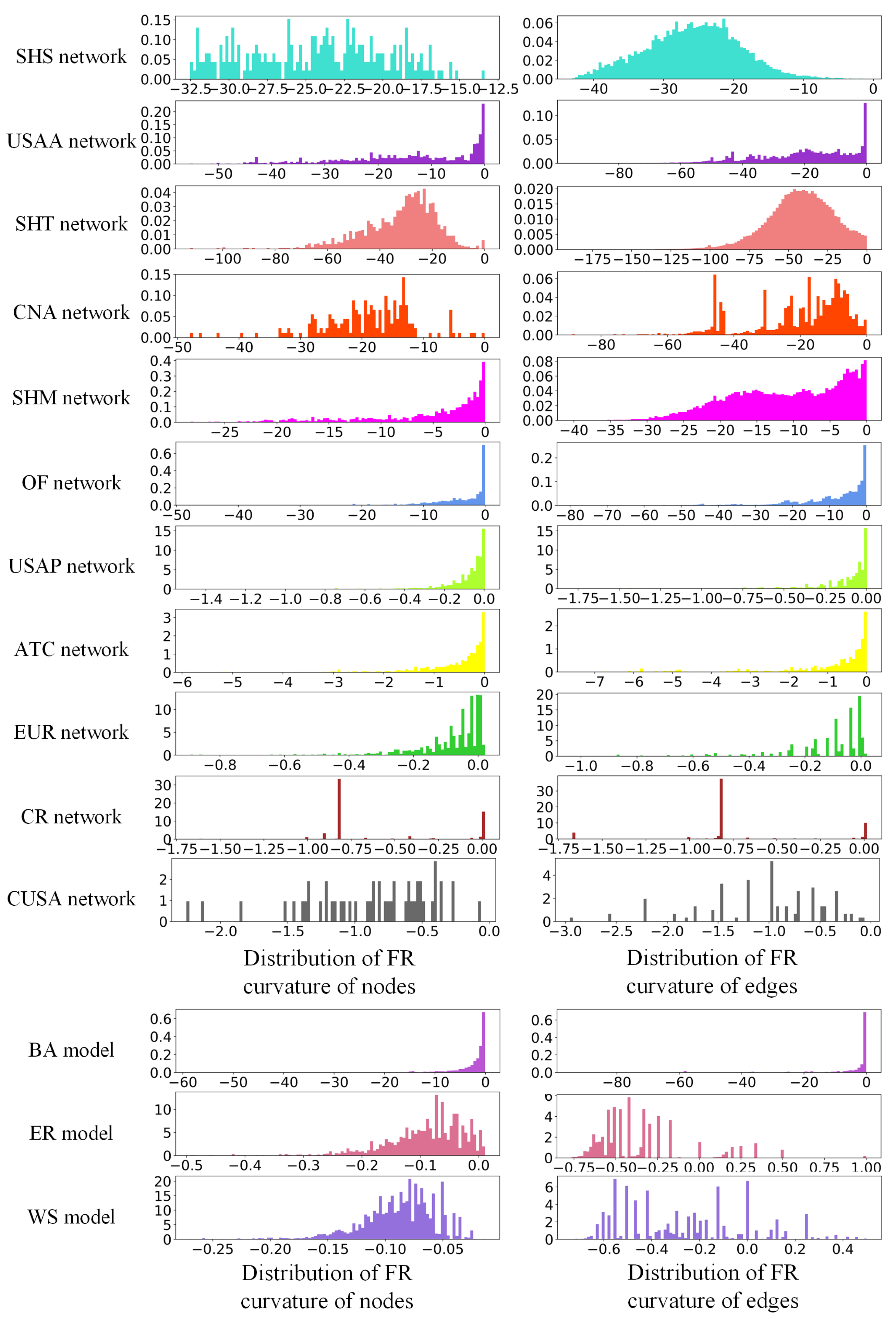
First, we compare the distribution law of the FR curvature in synthetic networks and real-world networks in Figure 1. We can see that the FR curvature distributions of half of the geographic networks are similar to the FR curvature distribution of the BA model network. The FR curvature distributions of the other networks are not similar to those of the three model networks. There are networks with a scale-free effect whose Ricci curvature distribution does not have similarities with those of BA model networks. The same problem also occurs in networks with a small-world effect.

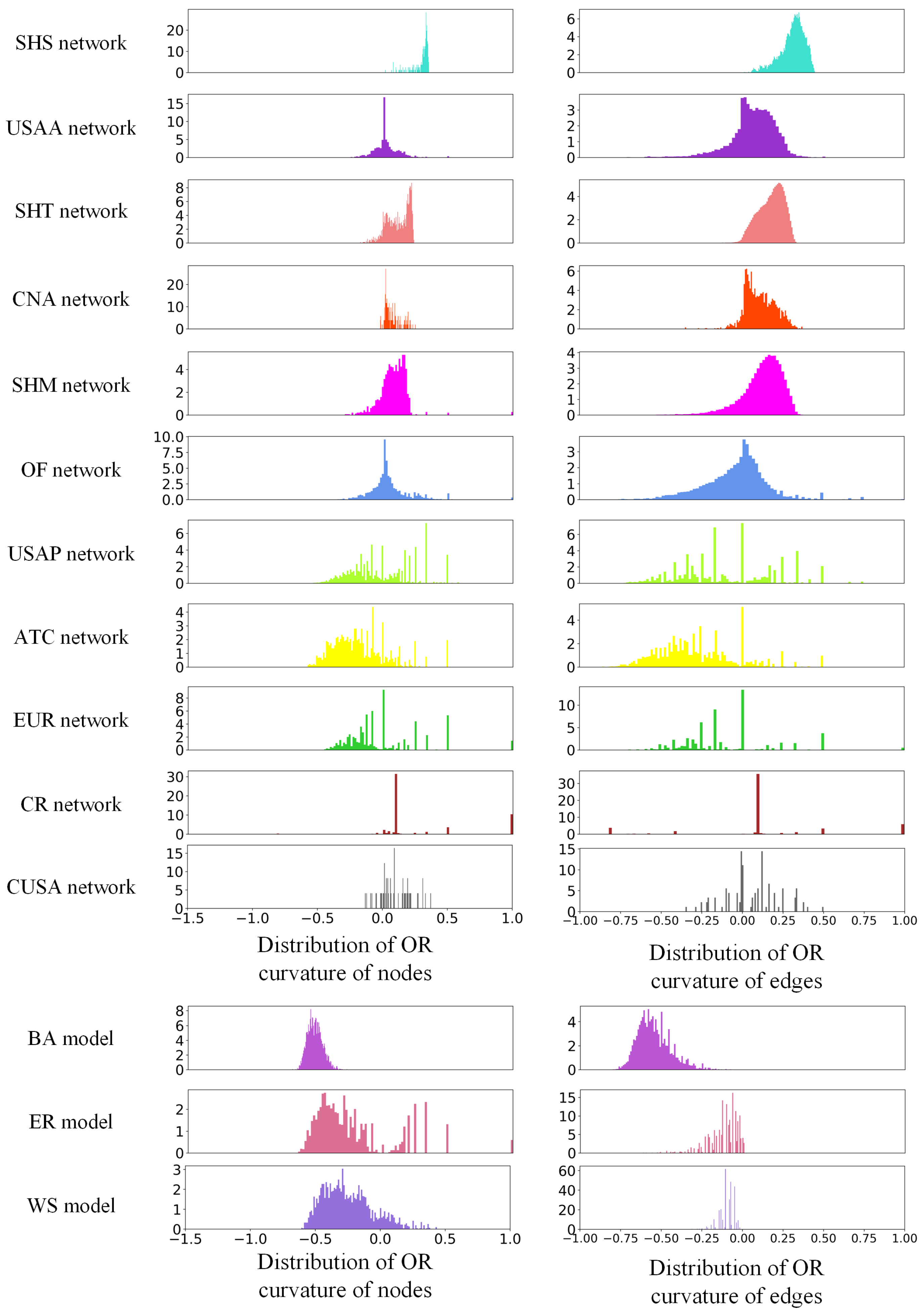
We also compared the distribution law of the OR curvature of synthetic networks and real-world networks. The results are shown in Figure 2. We found that the USAP, EUR, and OF datasets have a higher development potential than the other networks. The OR curvature distributions of USAA, CNA, USAP, SHM, OF, and ATC are similar to the distribution of the WS model network. It is impossible to distinguish whether the network has a scale-free effect by the distribution of the OR curvature.

To more intuitively understand the difference between the two kinds of Ricci curvature of geographic networks, we calculated the average Ricci curvature as a global characteristic. The results are shown in

Table 4. Global indicators based on the Ricci curvature.

Network	AFR_edge	AOR_edge	AFR_node	AOR_node
SHS network	−25.794	0.313	−24.329	0.293
USAA network	−20.257	0.069	−13.603	0.023
SHT network	−42.421	0.18	−31.917	0.116
CNA network	−20.064	0.112	−19.034	0.072
SHM network	−10.895	0.128	−5.327	0.081
OF network	−8.665	−0.036	−3.649	0.046
USAP network	−0.121	−0.103	−0.085	−0.011
ATC network	−0.862	−0.279	−0.549	−0.184
EUR network	−0.113	−0.106	−0.078	−0.016
CR network	−0.71	0.13	−0.573	0.281
CUSA network	−1.033	0.065	−0.877	0.101

. It can be found from Table 4 that the average FR curvature can refine the distinction between networks with the scale-free effect, and that the average OR curvature can explain the developability of a network.

Based on the above analysis, we can determine whether the two networks have structural similarities by comparing the Ricci curvature distributions of real-world networks. In addition, the FR curvature can refine and complement the scale-free effect of the network, while the OR curvature can serve as both a refinement and a supplement to the characteristics of the small world, and it can also measure the network’s development potential.

3.1.3. Network Analysis from the Algebraic Perspective

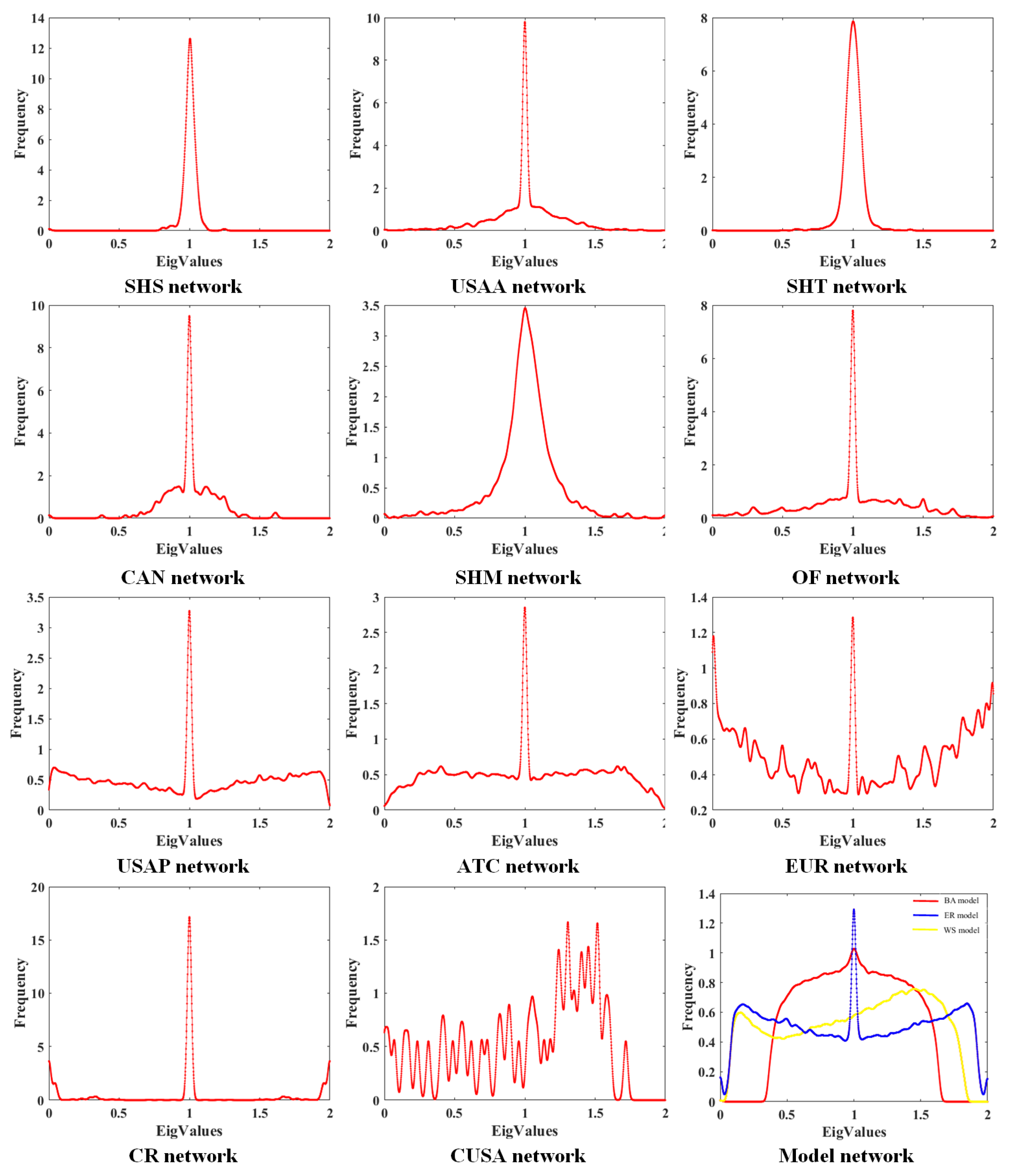
In this part, we have drawn the normalized Laplacian spectra of eleven geographic networks and three model networks and analyzed the structures of the studied networks from a macro perspective.

It can be seen from Figure 3 that networks with the small-world effect have similar spectral density distributions, while networks with the scale-free effect exhibit significant differences in spectral density distribution. The spectral distribution of most networks has a high degree of symmetry. Its peaks mainly appear near 1, and the eigenvalues in the interval of 0–2 are widely and densely distributed, indicating a rich and complex network structure. The spectral distributions of the model networks are very different from those of the real geographic networks, which indicate that the normalized Laplacian spectrum has a stronger ability to describe the network topology than the model network.

To quantitatively describe the global structure of the network, we calculated the algebraic connectivity $\alpha \left(G\right)$, motif multiplicity and spectral radius $\rho \left(G\right)$. The calculation results are shown in

Table 5. Algebraic connectivity, motif multiplicity and spectral radius reflected in the Laplacian spectrum of real networks.

Networks	$\mathit{\alpha }\left(\mathit{G}\right)$	$\mathit{\alpha }\left(\mathit{G}\right)$ Rank	Motif Multiplicity	Multiplicity Rank	$\mathit{\rho }\left(\mathit{G}\right)$	$\mathit{\rho }\left(\mathit{G}\right)$ Rank
SHS network	0.2711	3	0	9	2	1
USAA network	0.018	6	0.3183	3	2	1
SHT network	0.0623	4	0.0127	8	2	1
CNA network	0.3769	2	0.3385	2	1.6175	5
SHM network	0.8052	1	0	9	1.248	6
OF network	0.0145	7	0.2763	4	2	1
USAP network	0.0003	11	0.12	5	1.9917	2
ATC network	0.0127	8	0.0987	6	1.9861	3
EUR network	0.0005	10	0.0417	7	2	1
CR network	0.0016	9	0.5706	1	2	1
CUSA network	0.0291	5	0	9	1.7182	4

. It can be seen from Table 5 that the SHM network and the CNA network have higher algebraic connectivity, which means that neither of these two networks can be easily divided into two. The maximum eigenvalue verified this finding. A maximum eigenvalue close to 2 indicates that the graph is dichotomous. Motif multiplicity can explain the basic components of a network. We can see that four networks, i.e., the CR network, the CNA network, the USAA network, and the OF network, have the highest motif multiplicity, indicating that there are large numbers of star topologies in the basic topologies of these four networks. In other words, these networks have some high-degree nodes. The motif multiplicities are all zero in the SHM network, SHS network, and USATC network because the node degrees of these three networks are evenly distributed.

Based on the above analysis, we can see that the normalized Laplacian spectrum can reflect the overall structural information of a geographic network and information regarding the community structure, network constituent units and dichotomy that can be used to study the network structure.

3.2. Network Classification from Different Perspectives

In previous research, we found that different perspectives differ in their characterization of geographic networks. We can therefore qualitatively and quantitatively classify geographic networks based on the above studies.

3.2.1. Network Classification from a Single Perspective

Network classification criteria and results from different perspectives are displayed in

Table 6. Network classification criteria and results from different perspectives.

Network	Statistical			Geometric		Spectral					Class
	Small-World	Scale-Free	Class	AOR < 0	Class	Symmetry	Wide	Narrow	Irregular	Class
SHS	✓		STC1		GC1	✓		✓		SPC1	MC1
USAA	✓	✓	STC2		GC1	✓		✓		SPC1	MC1
SHT	✓	✓	STC2		GC1	✓		✓		SPC1	MC1
CNA	✓	✓	STC2		GC1	✓		✓		SPC1	MC1
SHM	✓	✓	STC2		GC1	✓		✓		SPC1	MC1
OF	✓	✓	STC2	✓	GC2	✓		✓		SPC1	MC1
USAP		✓	STC3	✓	GC2	✓	✓			SPC2	MC2
ATC		✓	STC3	✓	GC2	✓	✓			SPC2	MC2
EUR		✓	STC3	✓	GC2	✓	✓			SPC2	MC2
CR		✓	STC3		GC1	✓		✓		SPC3	MC3
CUSA			STC4		GC1			✓	✓	SPC4	MC4

. The principle for classifying networks from the statistical perspective mainly considers whether the network has a scale-free or small-world effect. Based on the content of Section 3.1.1, we can roughly divide the eleven networks considered in this article into four categories based on various statistical indicators. The average OR curvature can basically represent the global characteristics of a network, so we consider roughly classifying networks based on the average OR curvature. Based on the content of Section 3.1.2, we can roughly divide the eleven networks considered in this article into two categories. From the algebraic perspective, the basis for classifying networks is mainly the normalized Laplacian spectrum distribution. The eleven studied networks can be roughly divided into four categories according to the normalized Laplacian spectral characteristic values.

3.2.2. Network Classification from Multiple Perspectives

In previous research, we found that different perspectives in network analysis can complement each other so we can consider combining the three perspectives to qualitatively and quantitatively classify networks. Qualitative classification is mainly based on whether the network has scale-free or small-world effects, its Ricci curvature distribution, and whether spectrum distributions are similar. Quantitative classification is mainly performed by clustering the feature vectors of considered networks.

From the three perspectives, the eleven networks can be roughly classified into four categories from a qualitative perspective. The classification results are shown in Table 6 and the classification criteria are shown in

Table 7. Classification criteria from different perspectives.

Perspectives	Classes	Classification Criteria
Statistical	STC1	Neither a scale-free network nor a small-world network.
	STC2	With the small-world effect, without the scale-free effect.
	STC3	With both the small-world effect and scale-free effect.
	STC4	With the scale-free effect, without the small-world effect.
Geometric	GC1	With a positive AOR curvature, network is relatively completed.
	GC2	With a negative AOR curvature and high development potential.
Spectral	SPC1	With a concentrated eigenvalue distribution and distribution ranging beyond the 0∼2 interval.
	SPC2	With an eigenvalue distribution between 0 and 2 and symmetry at 1.
	SPC3	With a narrow distribution range and scattered.
	SPC4	With an irregular eigenvalue distribution.
Multiple	MC1	With the small-world effect, similar Ricci curvature distributions and concentrated but scattered eigenvalue distributions.
	MC2	With the scale-free but no small-world effect, negative average OR curvature and Laplacian spectrum symmetry at 1.
	MC3	With the scale-free effect and a widely distributed and dichotomous eigenvalue distribution.
	MC4	Neither the small-world nor scale-free effect, with average FR and OR curvatures both close to 0, asymmetrical spectral distribution.

. We can also perform cluster analysis on the network from a quantitative perspective. We choose the K-means clustering method to cluster the selected networks. The results are shown in

Table 8. Clustering results by K-means (K = 4).

Network	Qualitative	Quantitative
SHS	MC1	QT_MC1
USAA	MC1	QT_MC2
SHT	MC1	QT_MC3
CNA	MC1	QT_MC2
SHM	MC1	QT_MC2
OF	MC1	QT_MC2
USAP	MC2	QT_MC4
ATC	MC2	QT_MC4
EUR	MC2	QT_MC4
CR	MC3	QT_MC4
CUSA	MC4	QT_MC4

. We choose six statistical indicators, which include $ACC$, $ACC/AC{C}_{rand}$, $APL$, $APL/AP{L}_{rand}$, $\gamma$ and $AD$, six geometric indicators including the average Ricci curvature, maximum curvature, and minimum curvature; and three algebraic eigenvalues including the algebraic connectivity, motif multiplicity, and spectral radius to consist of the feature vector. As can be observed from the clustering results, the quantitative analysis subdivides the MC1 class in qualitative classification results, separates the SHS and SHT networks and merges the MC3 and MC4 classes into MC2. The quantitative classification scheme is basically the same as the qualitative classification scheme, demonstrating the high credibility of our qualitative study.

3.3. Invulnerability Analysis from Different Perspectives

The invulnerability evaluation of networks evaluates their ability to maintain large-scale connectivity under deliberate or random attacks. The invulnerability of a network is closely related to the inherent nature of the network itself. Therefore, this section will evaluate the invulnerability of different classes of urban geographic networks in the face of random and deliberate attacks. This experiment cannot only verify whether our classification criteria are consistent with the common sense but also provide certain method guidance for the fast determination of important nodes and important edges in the network.

3.3.1. Invulnerability Analysis Based on Nodes’ Attacks

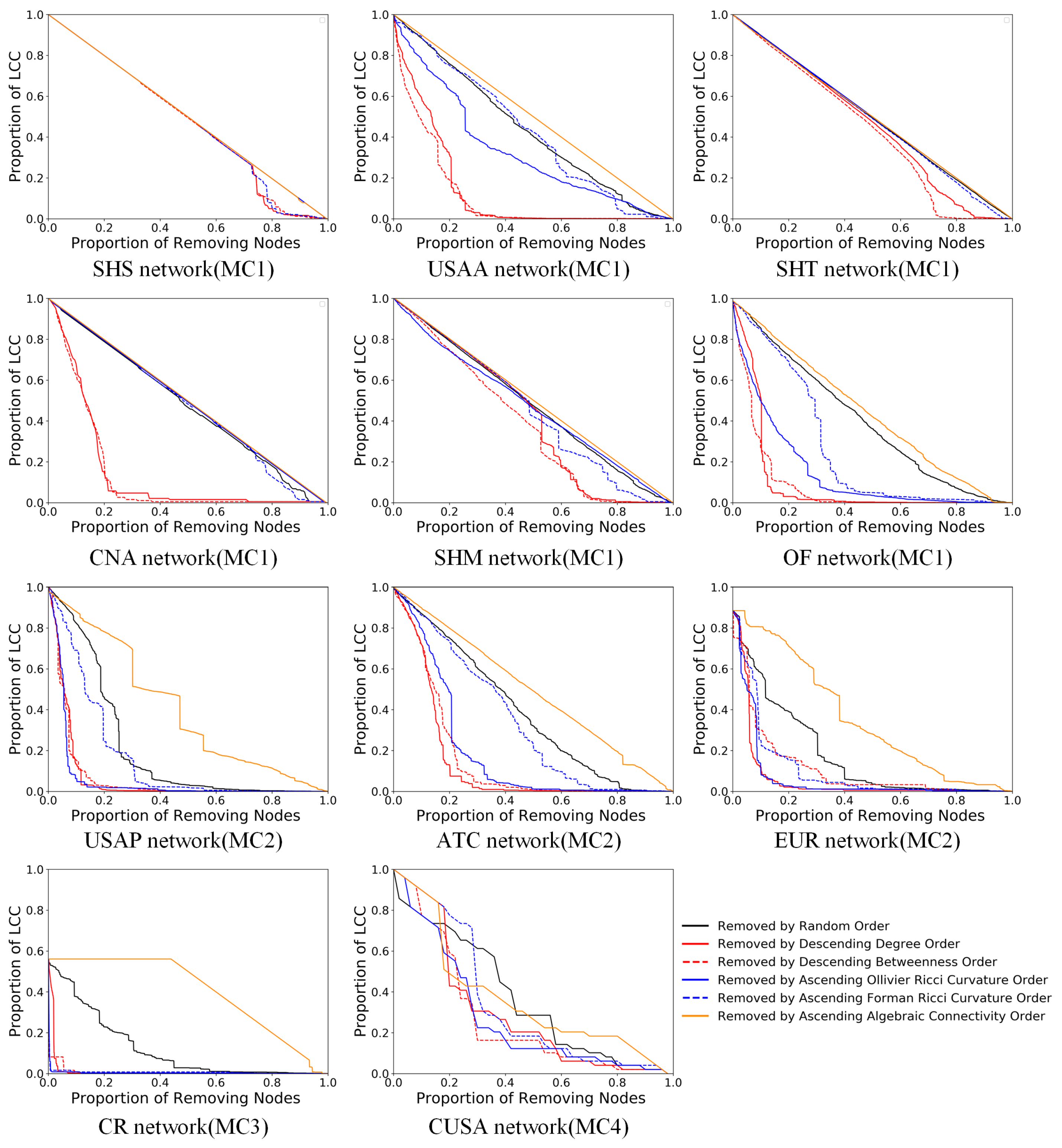
To verify whether the classification results based on the characteristics of the network structure have practical significance, we selected multiple indicators that can be used to measure the importance of nodes in the network from three perspectives and adopted two attack methods to attack nodes in geographic networks and model networks, namely random attack and deliberate attack. A random attack refers to randomly deleting nodes in a network. A deliberate attack refers to deleting nodes in a network in a certain order according to statistical indicators, geometric indicators and algebraic indicators. For the attacked network, we use the largest connected component (LCC) to represent the connectivity of the network. The relative size of the LCC is the ratio of the number of nodes owned by the maximal connected subgraph to the number of nodes in the original network.

We remove nodes in the network based on the following criteria: random order; order of increasing node FR curvature; order of increasing node OR curvature; order of decreasing node degree; order of decreasing node betweenness centrality; and order of increasing algebraic connectivity. The experimental results are shown in Figure 4.

The experimental results demonstrate that different types of networks perform differently in terms of invulnerability, indicating that our classification results have a certain reliability. In addition to analyzing the robustness characteristics of each type of network, we also compared the ability of the indicators to identify the important nodes from different perspectives. In maintaining the large-scale connectivity of the network, nodes with high node degree or high intermediate centrality are more important than nodes with high negative curvature, and nodes with high negative OR curvature are more important than nodes with high negative FR curvature. Algebraic connectivity cannot identify important nodes in the network.

3.3.2. Invulnerability Analysis Based on Edges Attacks

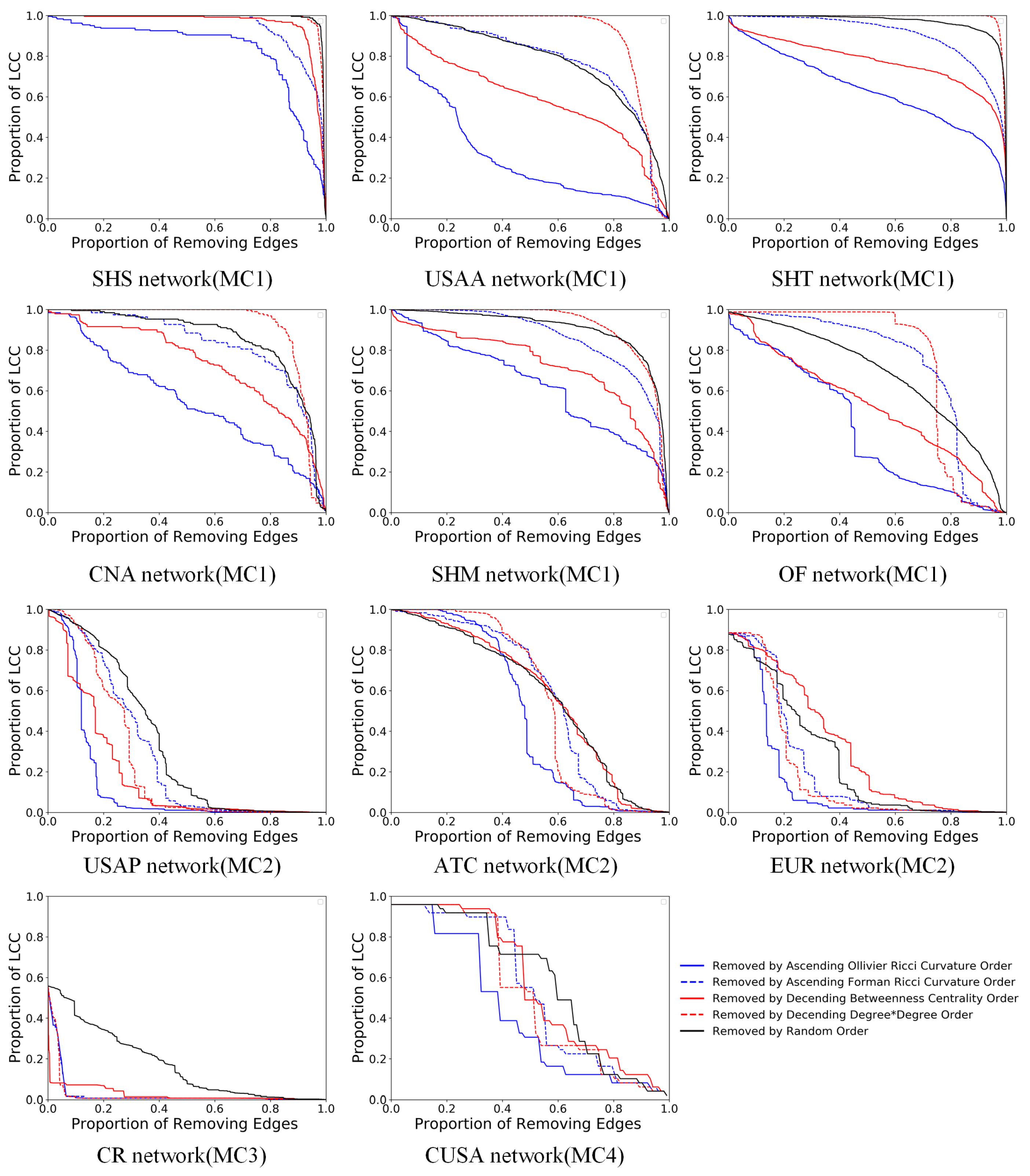
Unlike social networks, which are composed of physical nodes and virtual edges, geographic networks may have edges that exist in physical spaces, such as road networks. Therefore, in addition to the node attack experiments, we also examined the invulnerability of networks to edge attacks.

We removed edges from the network according to the following criteria: random order, order of increasing FR curvature of the edge, order of increasing OR curvature of the edge, order of decreasing point degree product at both ends of the edge, and order of decreasing centrality of the edge. The experimental results are shown in Figure 5.

In the edge deletion experiment, we observe that networks belonging to distinct classes exhibit significantly varying levels of invulnerability, indicating that our classification results have a certain reliability. In addition, we find that OR curvature indicators from the geometric perspective can quickly identify the important edges in the network.

4. Discussion

The geographic network analysis based on complex network theory is one of the hot topics in the field of geosciences. Numerous models and metrics have been developed to characterize the structural properties of networks. These models and metrics can be categorized into three categories: statistical perspective, geometric perspective and algebraic perspective. The majority of existing research explores the complex networks from a single perspective, resulting in one-sided analysis conclusions. In this paper, we simultaneously analyze the characteristics of geographic networks from three perspectives and propose network classification criteria from different perspectives. The topological invulnerability analysis of networks further verifies the classification results.

While statistical indicators can be used to determine whether a network exhibits the small-world or scale-free effect, we also discover that there can be significant variances between networks with identical statistical properties in reality.

As for the geometric perspective, OR curvature enables a more precise differentiation of the development stages of a network. We calculated two kinds of Ricci curvature for the nodes and edges in geographic networks and synthetic networks and found that, by comparing the Ricci curvature distributions of real networks and BA model networks, it is possible to further refine and distinguish networks with the same statistical characteristics.

From an algebraic perspective, the normalized Laplacian spectrum can reflect the overall structural information of geographic networks. It is found that real-world networks can be distinguished from synthetic networks by comparing the normalized Laplacian spectra.

These three types of perspectives capture the characteristics of geographic networks and the results generated from classification schemes based on different perspectives are inconsistent, indicating that various perspectives of complex network analysis complement each other. Moreover, we discover that statistical indicators outperform geometric indicators in identifying important nodes. In contrast, OR curvature based on the geometric perspective exceeds betweenness centrality based on the statistical perspective in finding important edges.

Finally, we propose a classification scheme based on multiple perspectives. The classification results can reveal the invulnerability of the geographic network to destruction under deliberate and random attacks, which can be helpful in urban planning and management. When constructing roads, for example, designers can use this scheme to determine whether the existing plan meets the requirement of invulnerability according to the category they are in and adjust the plan correspondingly.

5. Conclusions

Geographic systems are often modeled as complex networks to capture the essence of complex phenomena and processes. The key to obtaining the essential features is to explore the network’s structure. In characterizing the structure of complex geographic networks, researchers have proposed multiple metrics that can be classified into three major perspectives based on their mathematical theories: the geometric perspective, the statistical perspective and the spectral perspective.

In this study, we compared the different performances of the statistical, geometric and algebraic perspectives in synthetic networks and geographic networks. We found that the three types of perspectives are distinct in their characterization of network properties. Therefore, we propose a classification scheme considering all these three perspectives. In addition, we found that the statistical perspective focuses on the information of the important nodes in networks while the geometric indicators focus on the information of the edges in the networks. The findings regarding the focus of the three perspectives in the article can provide a reference for studying geographic network structure. When designing models for a downstream tasks, researchers can refer to geographic networks that belong to the same category under this classification scheme, and models may better transfer between the geographic networks of the same type.

However, the present study has a few limitations. In this study, the classification scheme is limited to unweighted and undirected geographic networks, while there are many weighted and directed ones in the real world. Moreover, with the rapid growth of complex network research in recent years, researchers from various domains have developed a variety of complex network analysis approaches from numerous perspectives, while only three dominant perspectives on the complexity of geographic networks were investigated in the present study; it is worth extending our work to the examination of whether other perspectives are appropriate for further geographic network analysis. Finally, it is worth mentioning that end-to-end deep learning methods have been widely used to extract features in remote sensing and transportation fields [37,38,39,40,41,42]. It undoubtedly also be helpful for geographic network analysis research.