1. Introduction
There is a wide variety of probabilistic models that have been proposed to analysis data generated from continuous random variables [
1,
2]. One of these models is the logistic distribution [
3]. Methods for estimating the parameters of some of these distributions have been well studied for different dimensionality of the parameter vector [
4].
The logistic distribution has been largely studied and generalized from different perspectives; see, for example, the works proposed in [
5,
6,
7,
8]. One of these models is the type I generalized logistic (IGL) distribution, which can be considered as a family of proportional reversed hazard functions with the logistic distribution being its base. The IGL distribution has been used to model data with an unimodal probability density function (PDF). For a comprehensive account of the theory and applications of logistic distributions, we refer the readers to [
2,
3,
9].
A three-parameter IGL distribution was proposed in [
10] and methods of estimation for its parameters were also presented in this work. The authors demonstrated that its log-likelihood function is strictly decreasing in one of its parameters, and maximized only when these parameters tend to infinity. Then, its maximum likelihood (ML) estimators do not exist and a hybrid method must be employed to optimize the log-likelihood function by plugging it at the posterior mean, but at the same time solving the problem of non-existence.
A technique for estimating the location and scale parameters of the IGL distribution was proposed in [
11] from a U-statistic constructed by using the best linear functions of order statistics as kernels. An efficiency comparison of the proposed estimators with respect to the ML estimator was also made by these authors. In a comparative study, the authors considered that there is an advantage when using a U-statistic for estimating the parameters from a practical point of view.
Some empirical evidence, based on stock markets and data sets of financial expected values, suggests that the true distribution of such expected values can be positively skewed in times of high inflation and more peaked than the normal distribution. The logistic distribution is often used in econometrics to model the consumer inflation rates due to its heavy tails compared to the normal distribution [
12]. Its generalizations, which additionally allow for asymmetries, have been applied to model extreme risks in the context of the German stock market [
13], and has been proved to be a simpler model than its harmonized index of consumer prices in inflation rates [
14].
A method for determining explicit estimators of location and scale parameters was proposed in [
15] by approximating the likelihood function using the Tiku method [
16]. An application in genomic experiments utilizing the IGL distribution to determine whether a gene is differentially expressed under different conditions was presented in [
17]. The authors simplified the computational complexity carrying out likelihood ratio (LR) tests for several thousands of genes. Moreover, an approximate LR test was also proposed to generalize the two-class LR method into multi-class microarray data. The IGL PDF can be symmetrical, left-skewed, right-skewed, and reversed-J shaped, which provides us with high flexibility in the modeling of the data.
The literature on the study of the performance of the joint estimators of the three-parameter IGL distribution is limited. Particularly for the ML estimators because, as mentioned, an estimation problem exists and the corresponding parameter space must be restricted for their existence. Despite this problem, an
R package named
glogis [
18] was published without further discussion about this problem [
19].
We can mention some other commonly used classical (or frequentist) estimation methods in addition to the ML approach. For example, we have the ordinary and weighted least squares methods [
20], which are defined in terms of order statistics, making these methods robust and helpful for estimating the parameters of a skew distribution. Also, other estimation approaches related to percentiles, minimum distances, and bootstrapping can be considered [
21]. Furthermore, the probability-weighted moment (PWM) method may be mentioned, which has been investigated by many researchers. This method was originally proposed in [
22], is commonly employed in theoretical and empirical studies, and has determined frameworks that are more stable against outliers. The PWM method may be generally used to estimate parameters of a distribution whose inverse form cannot be formulated explicitly. The L-moment method was introduced in [
23], which is linear combination of the PWM method. The L-moment method [
24] is more easily related to the distribution shape and spread than the PWM method. However, when estimating parameters, there is no reason to distinguish between the L-moment and PWM methods, because they lead to identical parameter estimates, at least for their usual settings. An
R package named
lmom [
25] has been implemented for the L-moment method.
When a distribution can be written as a mixture model [
26,
27], we may use the expectation-maximization algorithm proposed in [
28] to efficiently estimate its parameters. Nevertheless, this algorithm may present some disadvantages at the step of maximization due to the dependence on initial values for multimodal likelihood functions [
29]. To solve this and other issues discussed in the following sections, an alternative method based on a Bayesian approach was proposed in [
30], which is known as the stochastic expectation maximization algorithm. This algorithm includes a step of stochastic simulation based on the Gibbs sampling and the Metropolis–Hastings technique from the posterior distribution of the parameters, that is, it it takes prior information and utilizes it to deal with such disadvantages.
An approach based on importance sampling was used in [
31] to estimate the shape and scale parameters of the generalized exponential distribution, in addition to the Gibbs and Metropolis samplers to predict the behavior of the distribution. To the best of our knowledge, this approach has been not employed for the IGL distribution.
The main objective of this investigation is to use a Bayesian approach to obtain reliable estimators of the three-parameter IGL distribution. Specifically, we apply a Monte Carlo Markov chain (MCMC) algorithm to guarantee the coverage of the stationary distribution support. Our secondary objectives are: (i) to conduct a simulation study to assess the performance of some posterior distributional characteristics, such as the mean, utilizing Monte Carlo Markov chain methods; and (ii) to apply the proposed method to real-world data related to engineering area.
The outline of the paper is as follows.
Section 2 presents the three-parameter IGL distribution. In
Section 3, we introduce a classical approach to estimate the parameters of this distribution, whereas in
Section 4, we provide the numerical approximation of the posterior distributions to make Bayesian inference by using MCMC methods. In
Section 5, Monte Carlo simulation results are reported and discussed.
Section 6 applies the obtained results to a real-world data set from the area of copper metallurgical engineering to illustrate the potentiality of the Bayesian analysis in the three-parameter IGL distribution. Finally, in
Section 7, we sketch the conclusions of this study.
2. The Type I Generalized Logistic Distribution and Related Distributions
Let the random variable
W follow an IGL distribution with location (
), scale (
), and shape (
b) parameters. Then, the PDF and cumulative distribution function of
W are, respectively, given by
with
,
, and “e” denoting the exponential function. The family of IGL distributions consists of members with their positively skewed PDF and coefficient of kurtosis greater than that of the logistic distribution. If
W is an IGL distributed random variable, then
has a type II generalized logistic (IIGL) distribution [
32]. Additional generalizations of the logistic distribution are discussed in [
1]. For
, the distribution is symmetric, for
, it is skewed to the left (negative asymmetry), and for
, it is skewed to the right (positive asymmetry).
The moment generating function of the IGL distribution is stated as
where
is the usual gamma function defined as
, for
. From (
2), it follows that
with
and
being the digamma and trigamma functions, respectively. From the formulas established in (
3), the coefficient of skewness for
W, corresponding to the third standardized moment, is formulated as
Note that the expression given in (
4) does not depend on the parameter
.
For the sake of comparison of how flexible a generalized logistic distribution can be, when incorporating a fourth parameter, in relation to the IGL case, we introduce the type IV generalized logistic (IVGL) distribution with parameters
,
,
and
. If
, then we get
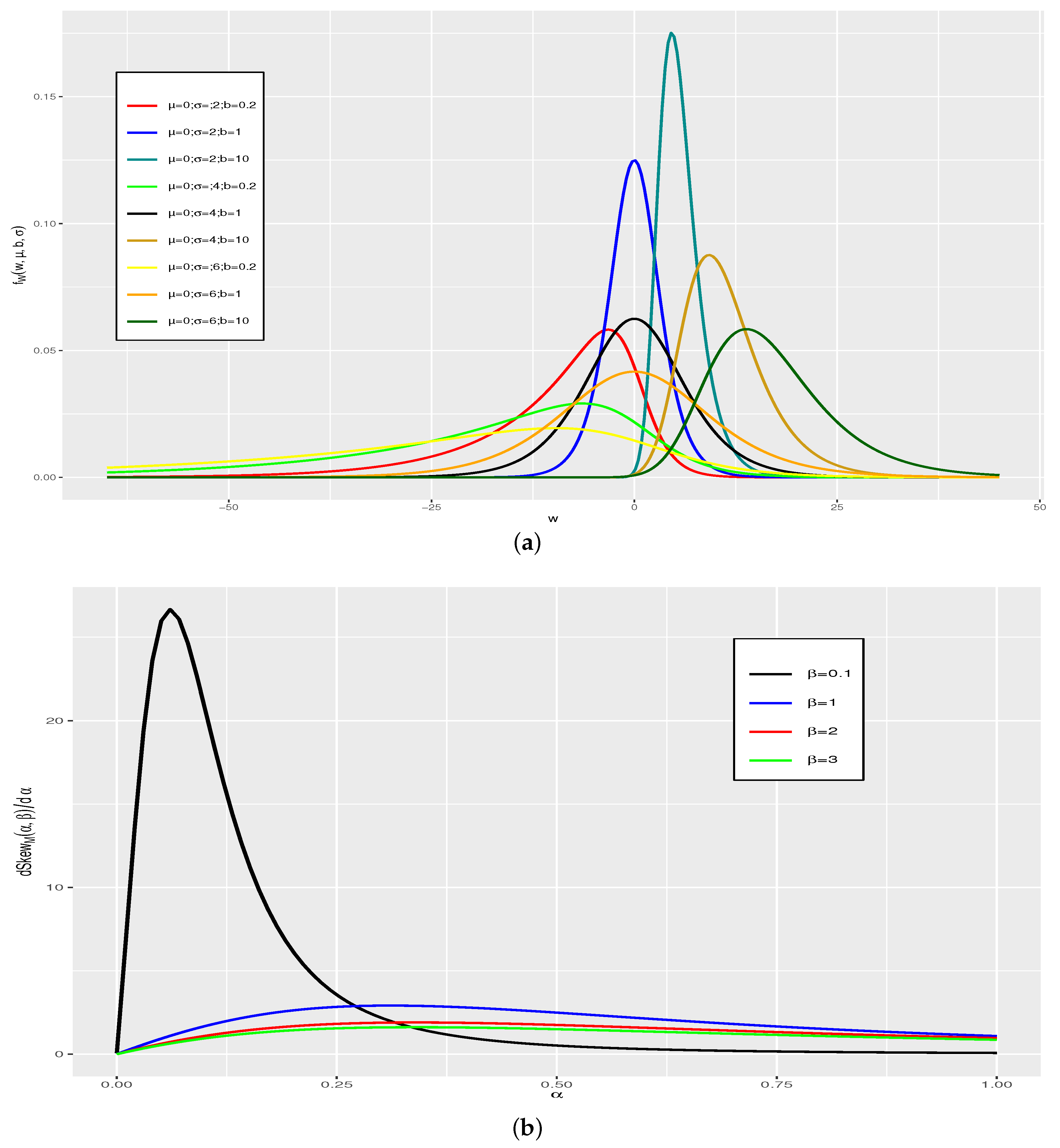
In
Figure 1a, we show the effect of the shape parameter
b for the IGL distribution, when the other parameters
and
take different values. It is clear from this figure that the distribution is negatively skewed for
and is positively skewed for
. The IGL distribution is flexible in the sense that the rate of change of the coefficient of skewness is greater for negative values than for the positive values in relation to the other generalized logistic distributions. In
Figure 1b, we show the flexibility to capture asymmetry of the IVGL distribution, which is more pronounced for values of the parameter
, approximately when
. Thus, this additional parameter of the IVGL distribution is not relevant. For the IIGL distribution, the skewness is a decreasing function of
b. Note that if the value of
b tends to infinity, then the IIGL distribution has heavier tails. We observe that the coefficient of skewness is approximately constant for values of the shape parameter greater than 0.025. Therefore, the IGL distribution can be used in robustness studies of classical procedures, since extreme values are often observed in real-world data.
3. Inference: Classical Approaches
Next, we describe the moment method of estimation. The expressions stated in (
3) are useful to find the moment estimators of
,
and
b,
,
and
namely, respectively. The estimator (moment-based) of Skew
for a sample
from the IGL
distribution is given by
If
, with
being defined in (
6), then it is possible to obtain a unique solution
from a condition stated as
Thus, over the condition given in (
7), we obtain the moment estimators for
and
by analytically solving the equations established as
Moreover, in [
10], note that
are consistent and asymptotically unbiased for
when
exists. However, from a practical numerical point of view, we see in our simulation study that the degree of sample asymmetry and the sample size affect the existence of
, without being sure of the restrictions for
, and so
does not satisfy the condition given in (
7).
Next, we consider the ML method of estimation. Assuming
is a sample of size
n from the IGL
distribution, the log-likelihood function of
is formulated as
, where
From (
8), we obtain a closed-form expression for estimating
b by the ML method, that is, we reach
with
. When plugging the estimator
into the log-likelihood function, we get the profile log-likelihood function, denoted in general by
(or concentrated log-likelihood function, whose terminology was borrowed from the ML theory, where the insertion of certain partial solutions
leads to such a concentration). Hence, the corresponding profile log-likelihood function is defined as
where
H is a function that does not depend on
given by
with
. Therefore, with a usual optimization algorithm to maximize the expression stated in (
10), we find the ML estimate
. However, the ML estimation in the IGL distribution has some problems. In [
10], it was shown that there is a path in the parameter space along which the likelihood function becomes unbounded.
We present the Fisher information matrix (FIM) of
in order to use it as a guide to define priori distributions for Bayesian inference on
. The FIM of
, say
, have elements given by
with
ℓ being the corresponding log-likelihood function. Thus, the FIM of
is stated as
, where
is the FIM when
, that is,
Note that the FIM is independent of
so that we can write
, with
. Moreover, we observe that, if
, difficulties appear when applying the Fisher asymptotic theory, having a singular FIM. Additional details can be found in [
33].
4. Inference: A Bayesian Approach
One of the first steps to do Bayesian statistics is generating information in terms of a PDF. Obtaining a priori distribution for a single parameter can be simple, if some experience in similar situations has been established. In the Bayesian inference, the posterior PDF
is constructed from the likelihood function
, and the prior PDF
for the parameters is obtained by means of what is known as the Bayes rule, that is,
In this context,
is known as the marginal likelihood function and is given by
which is often extremely hard to calculate when the likelihood function has a complex structure, as is the case when considering the IGL distribution. Hence, the Bayesian estimator of any function
g of
under squared error loss function is defined as
and under absolute error loss function, it is the median of
, that is,
Next, we conduct the prior specification. For a parameter vector, establishing a priori joint distribution can be much more complicated. It is also difficult to obtain information on the dependence of the parameters and express it in terms of a joint distribution.
We can consider a priori distribution for the parameter vector , say , as . Thus, by considering that each parameter is independent of the others, the last expression remains as .
The posterior PDF of
is, up to the constant factor
, stated as
where
with
and
acquiring the structures specified above (appropriate for its application). Therefore, the posterior PDF of
given the data is formulated as
Note that the integrals stated in the expressions defined in (
15) and (
18), as well as the solution of the equation established in (
16), are not simple to obtain explicit closed forms. Moreover, in this paper, we can specify the prior PDF without supposing independence between
,
and
b, via the Jeffreys prior. Note that the Jeffreys prior does not work well for models of multidimensional parameters [
34]. Nonetheless, we use it in the next section to find the Bayesian estimates in a particular case for the sake of comparison.
Next, we proceed with the MCMC estimation. We focus on those traditional tuned search procedures for proposed and associated priors. We test the method proposed in [
35], available for
R,
Python,
MatLab, and
C++. Using the
R language for our simulated scenarios here, it was not possible to achieve reasonable results.
Considering the MCMC algorithm, that is,
with distribution defined by
being accepted or rejected according to the MH algorithm, we set
where
is defined in (
17) and
q is a specific conditional PDF also called candidate kernel. Considering the likelihood functions previously defined, and the general prior specification given, the posterior distribution has a complex form. Then, the Bayesian estimation can be implemented by employing MCMC methods, which make it simpler to obtain efficient sampling from the marginal posterior distributions. A crucial step in designing an effective sampling regime, implemented in the acceptance/rejection step stated in (
20), is the choice of a kernel
q.
5. Simulation Studies
We recall that, for large samples, the biases of the ML and Bayesian estimators are negligible. However, for small and moderate sample sizes, the second-order biases of the ML estimators may be large. We use Monte Carlo simulation to evaluate the finite sample performance of the ML and Bayes estimators for the parameter
of the IGL distribution, with the PDF given in (
1).
In order to analyze the point estimation results from ML and Bayesian methods, we compute, for each sample size,
, each scenario specified, representing the degree skewness as: severe negative
–case 1–; moderate negative
–case 2–: zero
–case 3–; and moderate positive
–case 4–. For each of the two estimation procedures, it is reported the true bias (E
); the relative bias (
), by estimating E
with Monte Carlo experiments); and the root mean square error, that is,
, where MSE is the mean squared error estimated from the 5000 Monte Carlo replicates. The values of IGL distributed random variables were generated using the inversion method. More specifically, the generation of the random samples coming from
can be easily obtained utilizing the PDF defined in (
1) through the inverse transformation, that is, employing
, where
U is uniformly distributed on
. To find the ML estimate, the log-likelihood function defined in (
8) is maximized using the Newton–Raphson algorithm with first analytic and second derivatives, both implemented in the
glogisfit function of the
glogis package [
36].
To find the Bayesian estimate, we employ the MCMC algorithm by generating candidate
with probability
given in (
20). The Geweke and multivariate Gelman–Rubin criteria were used to evaluate convergence. Moreover, we utilize the Ljung-Box test to detect the autocorrelations in each chain.
Next, we conduct the classical estimation approaches. In order to show numerically the difficulties they have with the ML and moment methods when estimating the vector of parameters
, even if convergence is achieved in some replicates, we implement the methods with the generated simulations.
Table 1 reports the percentages of updates by means of the moment estimation. In addition, we apply the minimum chi-square estimation procedure [
37] implemented in [
38] for the
mipfp package of
R without achieving reliable results. We do not show these results in the paper due to restrictions of space.
Table 2 reports the results obtained for the estimates with the moment method and 1000 replicates for the size samples, cases, parameter, and indicators mentioned. These results are not satisfactory and, for the ML method, we do not report the results because they are totally unsatisfactory.
Now, the Bayesian approach is conducted. In the case where the parameter vector
of the IGL distribution incorporates the three parameters, that is,
,
and
b, we employ the traditional MCMC algorithm as an alternative to the classical estimation. Understanding the choice of prior distributions is undoubtedly the most controversial aspect of any Bayesian analysis [
39,
40], we proceed to specify two priori classes (informative and non-informative) for a parameter space of the IGL distribution.
We use the most common convergence criteria in the literature on the topic related to the Gelman–Rubin, Geweke, and Ljung-Box methods. The Gelman–Rubin statistic is built with at least two chains, where the variance is compared within and between them. If the variability is similar within the chains, they are considered to have converged. In terms of its practical use, the value of the statistic must be less that 1.2 [
41]. The Geweke test is constructed with a chain, which is usually done by taking the initial 10% and 50% of the chain and making a comparison of means between both partitions, where significant differences indicate that the chain does not converge. The Ljung-Box test is applied to each chain and tries to evaluate the correlation between chain values at different lags, in particular it was evaluated at a maximum of 15 lags. If there is any significant observed correlation, then the chain is correlated and is not considered a random sample. We employ the smallest
p-value of the 15 lags, if this is not significant. Then, the others correlations, for lags less than or equal to 14, are not significant either.
We consider a prior distribution given by where , and are specified as follows. For the case where we have severe negative skewness (case 1), we use , and . When we have moderate negative skewness (case 2), we assume , and -. When symmetry exists (case 3), we state , and . For the case of positive skewness (case 4), we employ , and as the dependent joint. We numerically test different priors and values of the hyperparameters to find the convergence of the chains and the sufficient number of iterations. Understanding that there are other methods to set hyperparameter values, for example, empirical Bayes and James–Stein estimators, the development and implementation of these other methods will be studied in future work.
The criterion for eliciting the kernels was mainly oriented to choosing those structures that allowed us to make the algorithm more efficient, that is, to decrease the rejection rate in the step that involves the Metropolis–Hastings ratio, as stated in (
20). Consequently for the simulation study, we have that:
Case 1: , ,
, ,
, .
Case 2: , ,
, ,
, .
Case 3: , ,
, .
Case 4: , ,
, ,
, ,
where ★ denotes the true value of the MCMC.
Next, we consider dependent and non-informative priors. A class of advisable priori distributions are of the non-informative type, whose construction method is relatively simple, and without privileging specific behavior for any element of the parameter vector. This can be achieved via a Jeffreys prior defined as
where
is defined with the elements given in (
12), and
. We observe that the behavior of the Jeffreys prior depends only on
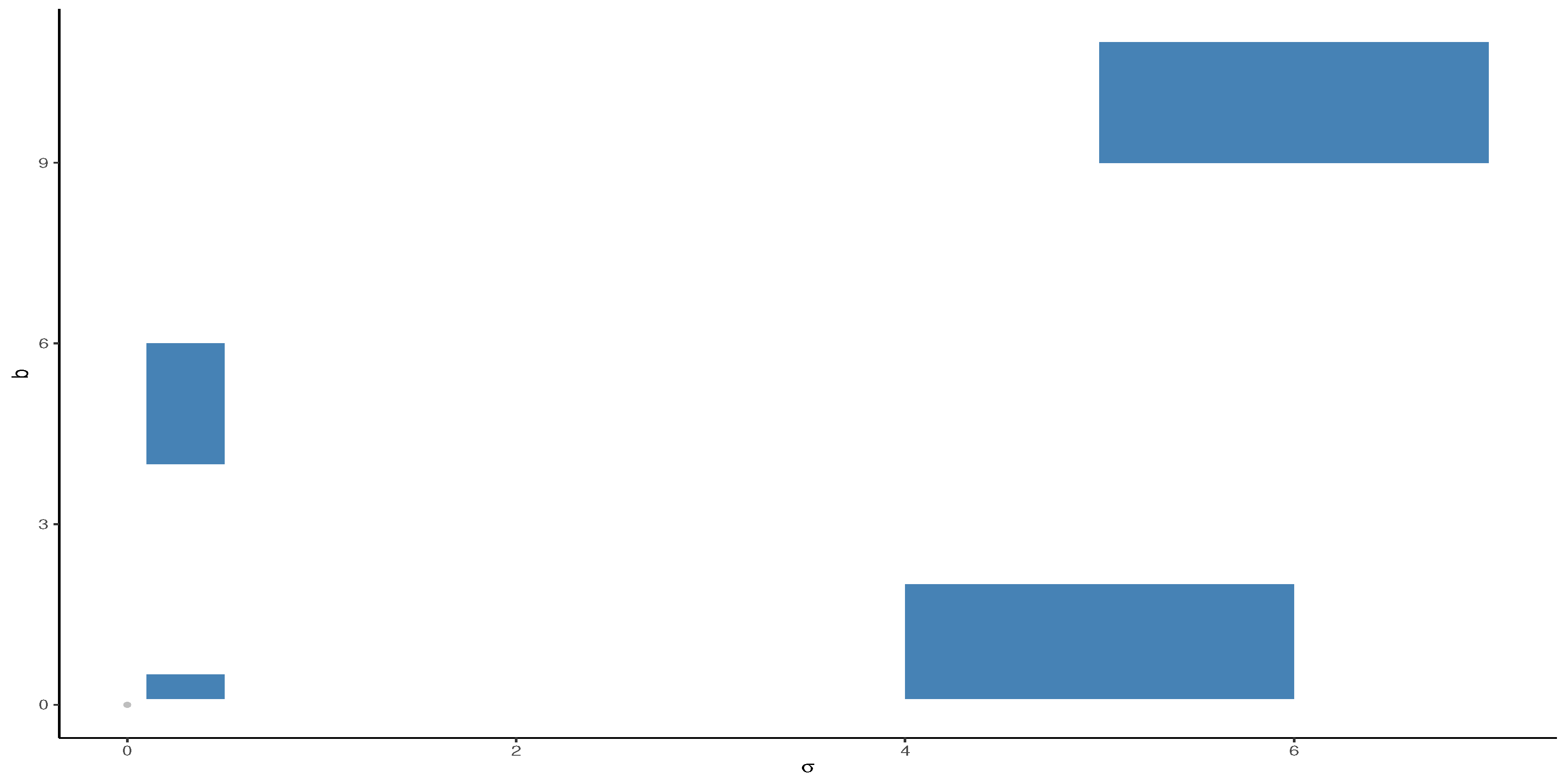
. In
Figure 2, we show the behavior of
on the subspace of
, say
, highlighting four region: (a)
; (b)
; (c)
; and (d)
. Thus, in general, note that the PDF of a Jeffreys prior takes extreme values when the scale parameter (
) is close to the origin and in greater degree when the shape (
b) is close to the origin (see
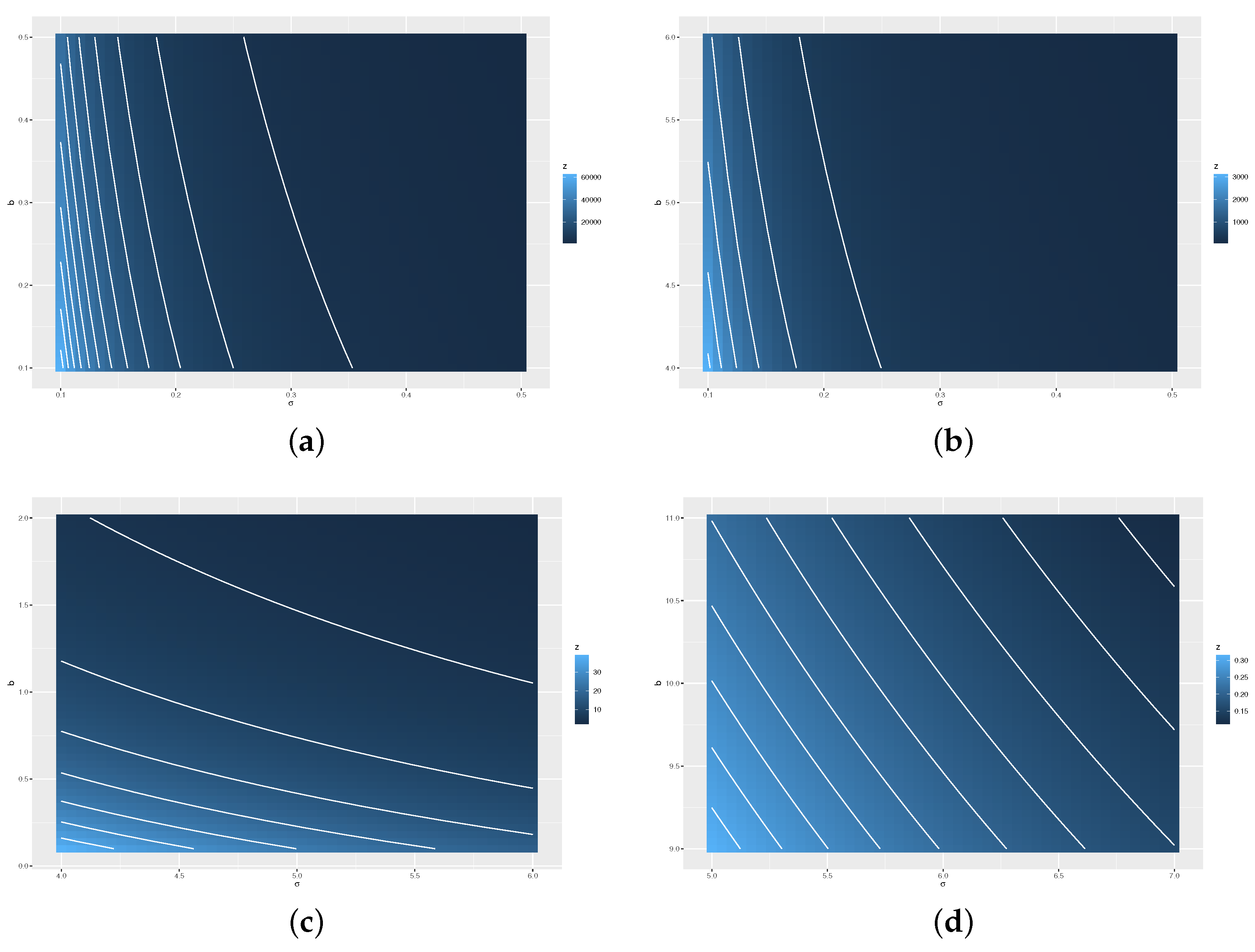
Figure 3a,b, respectively). Whereas if we move away from it (see
Figure 3c,d), the Jeffreys prior PDF (in this figure denoted as
z) takes smaller values. This is the reason why it is recommended to use it in cases where empirical asymmetry is positive, that is,
, in order to avoid those parts of the domain where the PDF has very strong changes and thus damages the efficiency of the algorithm. The above does not disregard the use of the independent and non-informative priors. To achieve a reasonable rejection rate, these results indicate to us that a Jeffrey priori on the region (c) should be considered.
Table 3 and
Table 4 report the results obtained for the posterior mean and median estimates, respectively, with the Bayesian method and 1000 replicates for the size samples, cases, parameter, and indicators mentioned. These results are quite satisfactory and helpful. We use the convergence Gelman–Rubin, Geweke, and Ljung-Box criteria, with their results being reported in
Table 5. From these results, we observe that all criteria employed here tell us that all chains converge, except, although debatable, in the case where the distribution has a severe negative skewness and with a small sample size. In a future study, we hope to provide a detailed discussion on the selection of priori distributions. We recall that the main objective of our study is to show that the Bayesian estimation is an alternative to the estimation problem of the three-parameter IGL distribution.
6. Empirical Application
Next, we present an application of real-world data corresponding to the solvent extraction (SX) process of copper. This process considers several stages of extraction and re-extraction with their respective operating variables. These variables, as in any process, often generate difficulties to the operation as the lack of efficiency on the copper recovery itself. Generally, difficulties occur in the following stage—the electrowinning (EW). Thus, it results from the dragging of unwanted impurities into the electrolyte. One of the purposes in the metallurgical area is to analyze the process in the stages of solvent extraction and electro-obtaining, identifying the most relevant variables, according to their: (i) impact on the process; (ii) empirical and design operational conditions; and (ii) parameters of control. The pregnant leach solution (or impure aqueous solution, known as PLS in short), from the leaching process, feeds the SX area which, by an organic solvent, is transferred to a pure and concentrated copper sulfate solution, called rich electrolyte, which is sent to the electro-obtaining area. The total PLS flow that feeds the plant is one of the main factors that determine the efficiency of copper extraction [
42].
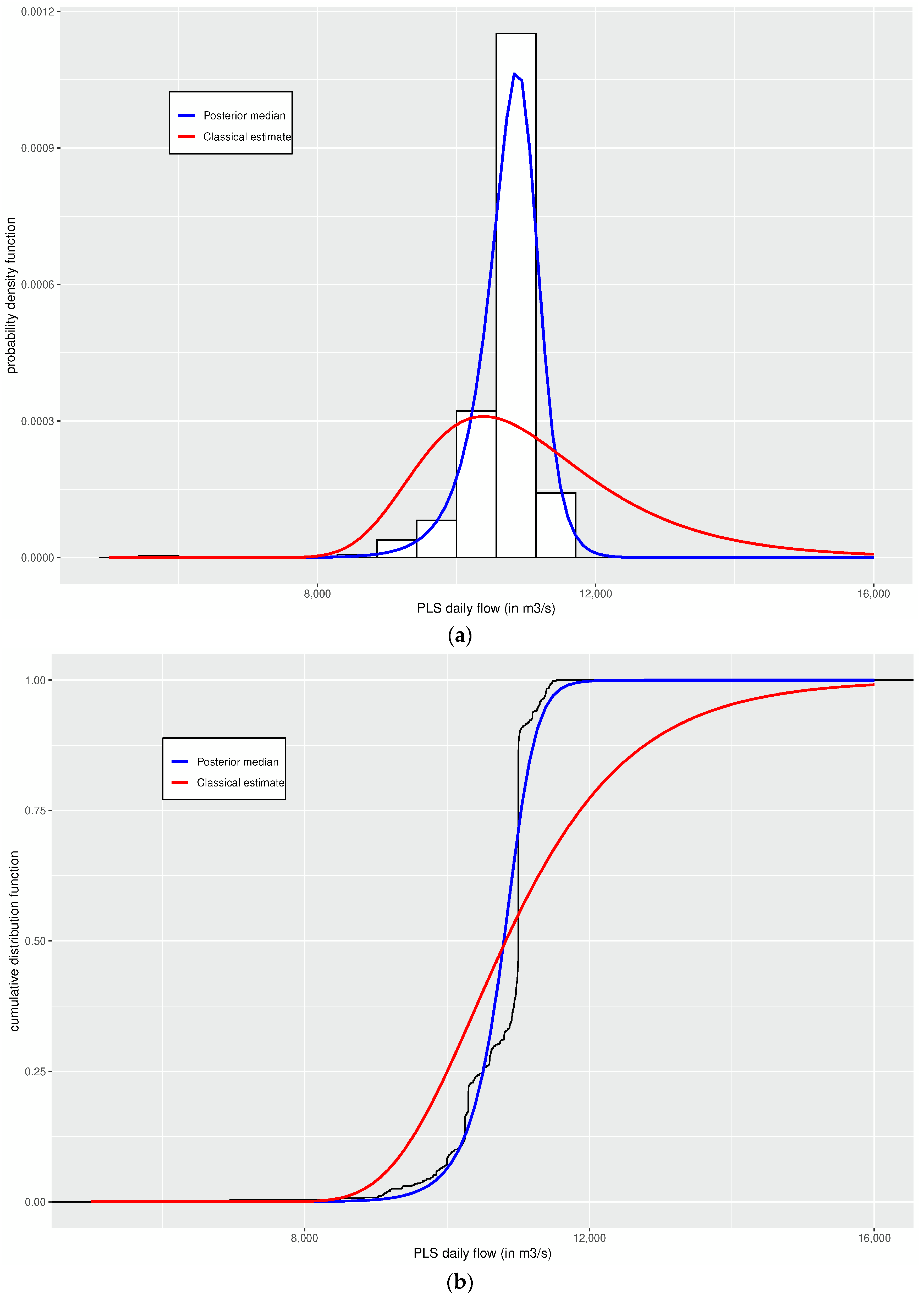
The PLS daily flow throughout the extraction process in the area of SX sulfides (
W) was registered between years 2015 and 2019, with a sample size of
. A descriptive summary, a histogram and the empirical cumulate distribution of the data set are shown in
Table 6 and
Figure 4, respectively. We can observe from
Table 6 and
Figure 4 that the data distribution has a moderate positive skewness. This is a very complex situation to estimate the parameters of the IGL distribution by the moment and ML methods, as it was shown in
Section 2 and simulation study of
Section 4. We use the Bayesian estimation method.
To apply Bayesian estimation, we consider independent and informative prior distributions for the parameter and , where and The hyperparameters are set by utilizing the criteria mentioned. For the kernels, we have:
E, Var,
E, Var,
E, Var.
In the diagnostic analysis, we have that the multivariate Gelman–Rubin factor is 1.01. The
p-values from the Geweke test are in
Table 7, from where we can observe that, only for the chains associated with the shape parameter
b, this was significant at 5%. Moreover, in
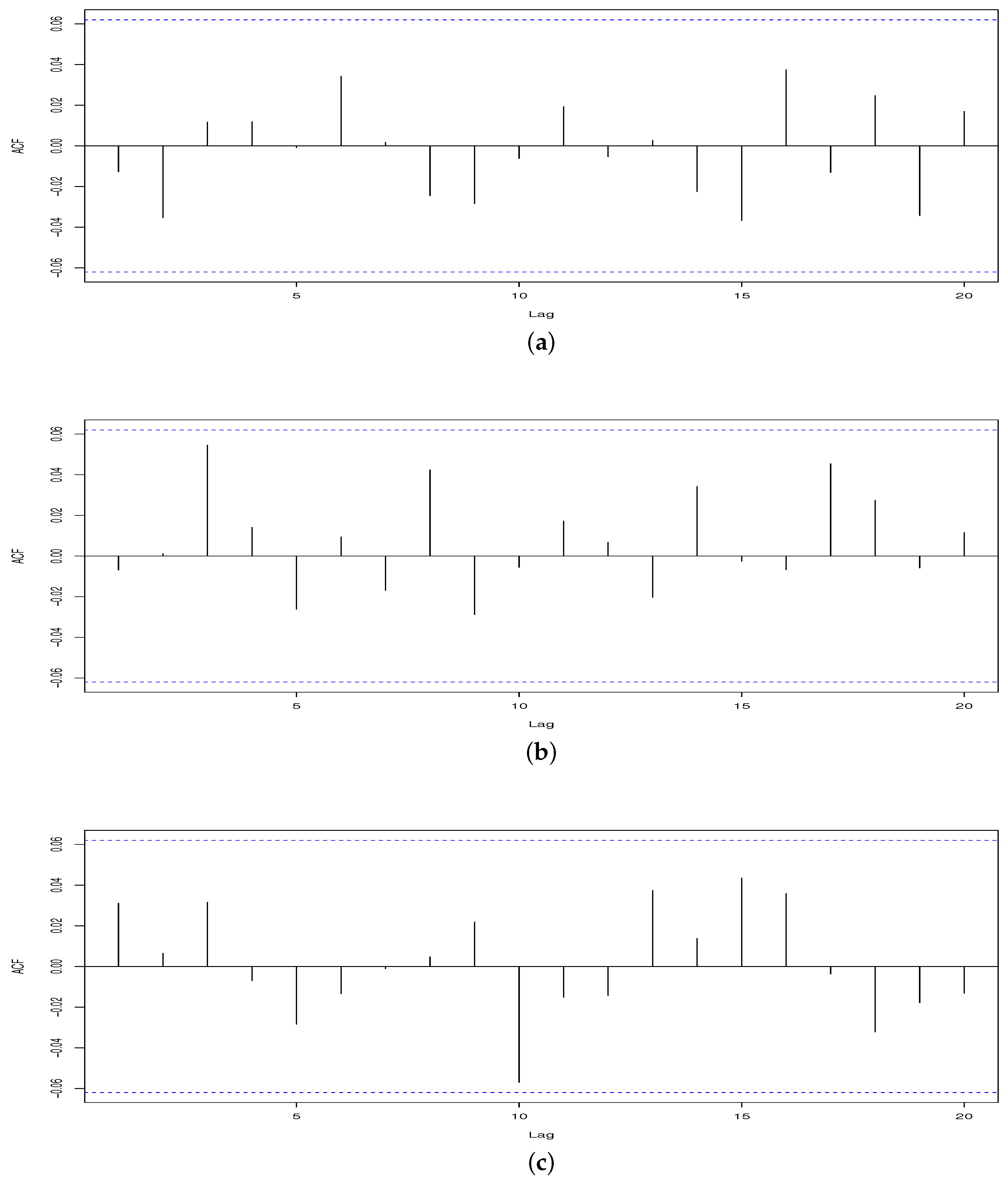
Figure 4, the histogram with the fitted IGL PDF (a) and the empirical cumulate distribution with the fitted IGL cumulative distribution function (b) are shown, from where we can see that a good fit was achieved in comparison to the other estimation methods considered in this article. The Bayesian estimate of
is reported in
Table 8, and the autocorrelation functions (ACFs) of the chains are shown in
Figure 5. Thus, by having the daily flow distribution of the PLS characterized via the estimated values of the parameters, and the solvent extraction process, the entire LX-SX-EW circuit is better controlled since the behavior of the PLS flow is better characterized. In this way, the control becomes more efficient.


 ,
, 


