Stability and Bifurcation Analysis of a Nonlinear Rotating Cantilever Plate System

Abstract

This paper investigates the bifurcation behavior and the stability of the rotating cantilever rectangular plate that is subjected to varying speed and centrifugal force. The local stability of the degenerated equilibrium of nonlinear system with symmetry is observed after analyzing the corresponding characteristic equation. In addition to complex phenomena such as static bifurcation and Hopf bifurcation, the 2-D torus bifurcation is investigated in this paper. Thereafter, the steady-state solutions and stability region are obtained using the center manifold theory and normal form method. Finally, numerical simulations are conducted to show the nonlinear dynamical behaviors of the rotating cantilever rectangular plate.

1. Introduction

With the rapid development of science and technology, many materials with outstanding and specific properties have appeared. Functionally graded materials (FGM) is a new kind of composite material whose composition and structure change continuously composed of two or more materials [1]. Recently, FGM has become more widely used in the aerospace industry and other fields, and its related research and application have grown rapidly, making it one of the research hotspots in the field of materials both at home and abroad.

Wang and Zu [2] studied the geometric nonlinear vibration problem of S-FGM plates. Based on D’Alembert’s principle, they derived the nonlinear motion equation of S-FGM plates, discretized and solved the motion equation, and studied the stability of the steady-state solution. Reddy [3] developed a finite element model of functionally graded material plates with changes in thickness direction using the high-order shear deformation plates theory and von Karman’s large deformation theory. Guo et al. [4] developed a nonlinear dynamic equation for four-sided simply supported fiber-reinforced composite laminates under the combined action of x-axis plane excitation and transverse excitation, and studied the dynamic behavior of its average equation. Wu [5] established the nonlinear dynamic equation of functionally gradient material rotating cantilever plate with variable rotation speed and analyzed the dynamic behavior of its average equation. Li et al. [6] obtained the four coupled nonlinear differential equations of FGM shell using new displacement field and analyzed the nonlinear transient dynamical behavior of the system. Sitli et al. investigated the buckling and post-buckling behaviors of FGM plate using the asymptotic numerical method [7], and meshfree radial point interpolation method [8].

Zhang et al. [9] investigate the local stability and bifurcation behavior of simply supported FGM rectangular plates in a uniform thermal environment by transverse and plane excitation, and three types of critical points of the system are discussed. It is found that the theoretical analysis is consistent with the numerical simulation, which is given with the help of Runge–Kutta method. Sharm et al. analyzed the bifurcation and stability behavior of the cholera model using the compound matrix technique [10,11]. Huseyin et al. studied the bifurcation and stability behavior of the nonlinear dynamical systems using unified technology and the critical point of the bifurcation response equation is defined by a simple zero, and a pair of purely imaginary eigenvalues [12], and two different pairs of purely imaginary eigenvalues [13], etc. [14,15]. Cai et al. [16] discussed the local stability switches and Hopf bifurcation of modified Van der Pol–Duffing equation using the $\tau$-decomposition method and center manifold theory.

A perturbation method for calculating the normal form is proposed in references [17,18,19,20]. Combined with the multi-scale method, the unique normal form of the given nonlinear dynamic systems can be obtained. Meanwhile, several physical models are given to verify the method. Algaba et al. [21,22] analyzed the orbital normal form of the nondegenerate Hopf-zero singularity and applied the results to discuss the three-dimensional Fitzhugh-Nagumo system. Kincaid and Cheney [23] discussed the Runge-Kutta method of order four, which is a high-precision algorithm widely used in engineering and is often used to numerically solve differential equations. When using computer simulation, this method saves the complex process of solving differential equations. Moreover, it has higher accuracy than Euler method and second-order Runge–Kutta method. In recent years, many scientists have proposed various methods for numerical simulation of nonlinear equations. Huang et al. [24,25] presented an incremental harmonic balance method to discuss the quasi-periodic response of the Van del Pol–Matheieu equation. Although these methods are in good agreement with fourth-order Runge–Kutta method in numerical simulation, the fourth-order Runge–Kutta method can better realize the numerical simulation on computer because its algorithm is relatively mature and its calculation accuracy is higher.

The contribution of this paper is the discovery of the complex nonlinear phenomena of the rotating cantilever plate system for the 1:1 internal resonance, principal parameter resonance, and 1/2 subharmonic resonance. By utilizing the normal form theory, the complex rotating cantilever plate system is simplified to its normal form which is qualitatively equivalent to its original system. Using the bifurcation theory, and stability theory, we discuss three types of degenerate equilibrium points and obtain the stability conditions and transition curves of the static bifurcation, Hopf bifurcation, and bifurcation of the two-dimensional torus. As we all know, the bifurcation will lead to harmful dynamic behavior of rotating cantilever plate system and make the system lose its original structural stability. Therefore, it is essential to select appropriate parameters of the rotating cantilever plate system. The findings show that the numerical and analytical results are essentially consistent.

The rest of the paper is organized as follows. In Section 2, the averaged equations of the motion of a functionally graded material rotating cantilever plate at variable speed and as well as the stability conditions of its initial equilibrium solution are given. In Section 3, the stability and the bifurcation analysis of the system near the three degradation equilibria are presented. In Section 4, some concluding remarks are made.

2. Problem Formulation

This paper focuses on the bifurcation and stability behaviors of the rotating cantilever FGM plate subjected to varying speed and centrifugal force. Figure 1 depicts a rotating cantilever FGM plate with dimensions $a$, $b$, and $h$. The rotational speed has the formula ${\mathsf{\Omega }}_r={\mathsf{\Omega }}_0+fcos\left(\mathsf{\Omega }t\right)$, where $f$ and $\mathsf{\Omega }$ are the amplitude and frequency of the velocity disturbance.

Figure 1. The model of rotating cantilever rectangular plate.

Using the Reddy’s high-order shear deformation theory, Hamilton’s principle and Galerkin’s method, the symmetric nonlinear dimensionless two-degree-of-freedom symmetry system of rotating cantilever FGM plate is written as follows [5],

$$\begin{array}{c}{\ddot{\omega }}_1+\left(g_1+f_{11}\mathit{sin}\left(\mathsf{\Omega }t\right)\right){\omega }_1+\left(g_2{\mathsf{\Omega }}_0+f_{12}\mathit{cos}\left(\mathsf{\Omega }t\right)\right){\dot{\omega }}_1+g_3{\omega }_1^2+g_4{\omega }_1{\omega }_2+g_5{\omega }_1{\omega }_2^2+g_6{\omega }_1^2{\omega }_2+g_7{\omega }_1^3+\\ g_8{\omega }_2^2+g_9{\omega }_2^3+\left(g_{10}+f_{13}\mathit{sin}\left(\mathsf{\Omega }t\right)\right){\omega }_2+\left(g_{11}+f_{14}\mathit{cos}\left(\mathsf{\Omega }t\right)\right){\dot{\omega }}_2+g_{12}{\ddot{\omega }}_2=0,\end{array}$$

(1a)

$$\begin{array}{c}{\ddot{\omega }}_2+\left(h_1+f_{21}\mathit{sin}\left(\mathsf{\Omega }t\right)\right){\omega }_2+\left(h_2{\mathsf{\Omega }}_0+f_{22}\mathit{cos}\left(\mathsf{\Omega }t\right)\right){\dot{\omega }}_2+h_3{\omega }_2^2+h_4{\omega }_1{\omega }_2+h_5{\omega }_1{\omega }_2^2+h_6{\omega }_1^2{\omega }_2+h_7{\omega }_2^3+\\ h_8{\omega }_1^2+h_9{\omega }_1^3+\left(h_{10}+f_{23}\mathit{sin}\left(\mathsf{\Omega }t\right)\right){\omega }_1+\left(h_{11}+f_{24}\mathit{cos}\left(\mathsf{\Omega }t\right)\right){\dot{\omega }}_1+h_{12}{\ddot{\omega }}_1=0,\end{array}$$

(1b)

where all the coefficients can be found in reference [5]. Using the asymptotic perturbation method, the average equation of the system in rectangular coordinates with symmetry is obtained as follows

$${\dot{x}}_1=\left(-{\mu }_1{\mathsf{\Omega }}_0+{\alpha }_1\right)x_1+{\sigma }_1{x}_2+\left(-{\mu }_2{\mathsf{\Omega }}_0+{\alpha }_3\right)x_3+{\alpha }_2{x}_4+N{g}_1^1,$$

(2a)

$${\dot{x}}_2=-{\sigma }_1{x}_1-\left({\mu }_1{\mathsf{\Omega }}_0+{\alpha }_1\right)x_2+{\alpha }_2{x}_3-\left({\mu }_2{\mathsf{\Omega }}_0+{\alpha }_3\right)x_4+N{g}_2^1,$$

(2b)

$${\dot{x}}_3=\left(-{\mu }_4{\mathsf{\Omega }}_0+{\beta }_3\right)x_1-{\beta }_2{x}_2+\left(-{\mu }_3{\mathsf{\Omega }}_0+{\beta }_1\right)x_3+{\sigma }_2{x}_4+N{g}_3^1,$$

(2c)

$${\dot{x}}_4={\beta }_2{x}_1-\left({\mu }_4{\mathsf{\Omega }}_0+{\beta }_3\right)x_2-{\sigma }_2{x}_3-\left({\mu }_3{\mathsf{\Omega }}_0+{\beta }_1\right)x_4+N{g}_4^1,$$

(2d)

where ${\omega }_1$ and ${\omega }_2$ are two different linear frequencies, ${\sigma }_1$ and ${\sigma }_2$ are two different detuning parameters, ${\mu }_i$ are damping parameters. The nonlinear functions $N{g}_i^1$ can be found in reference [5].

The Jacobi matrix of symmetric system (2) at equilibrium point $E=\left(x_1,x_2,x_3,x_4\right)=\left(0,0,0,0\right)$ takes the following form:

$$A=\left[\begin{array}{cccc}-{\mu }_1{\mathsf{\Omega }}_0+{\alpha }_1& {\sigma }_1& -{\mu }_2{\mathsf{\Omega }}_0+{\alpha }_3& {\alpha }_2\\ -{\sigma }_1& -\left({\mu }_1{\mathsf{\Omega }}_0+{\alpha }_1\right)& {\alpha }_2& -\left({\mu }_2{\mathsf{\Omega }}_0+{\alpha }_3\right)\\ -{\mu }_4{\mathsf{\Omega }}_0+{\beta }_3& -{\beta }_2& -{\mu }_3{\mathsf{\Omega }}_0+{\beta }_1& {\sigma }_2\\ {\beta }_2& -\left({\mu }_4{\mathsf{\Omega }}_0+{\beta }_3\right)& -{\sigma }_2& -\left({\mu }_3{\mathsf{\Omega }}_0+{\beta }_1\right)\end{array}\right].$$

(3)

Calculating the characteristic polynomial of (3), we have

$$f\left(\lambda \right)={\lambda }^4+b_1{\lambda }^3+b_2{\lambda }^2+b_3\lambda +b_4,$$

(4)

where the parameters $b_i\left(i=1,2,3,4\right)$ are elided. According to the Hurwitz criterion, one can also argue that while

$$b_1>0,b_1{b}_2-b_3>0,b_4>0,b_3\left(b_1{b}_2-b_3\right)-b_1^2{b}_4>0,$$

(5)

We get $E$ is stable, otherwise, $E$ is unstable and bifurcation may occur. The parameter values affect the stability of the equilibrium point.

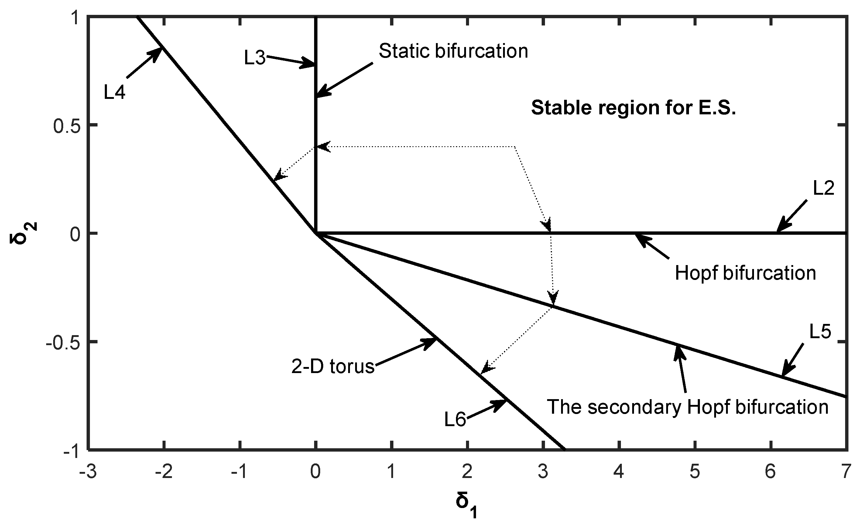
3. Bifurcation and Stability Analysis

In this section, we consider Equation (2) and turn to the local stability and bifurcation analysis of equilibrium points. The values of the two damping parameters ${\mu }_1$ and ${\mu }_3$ will be varied to study the effects on the system (2) that has symmetry.

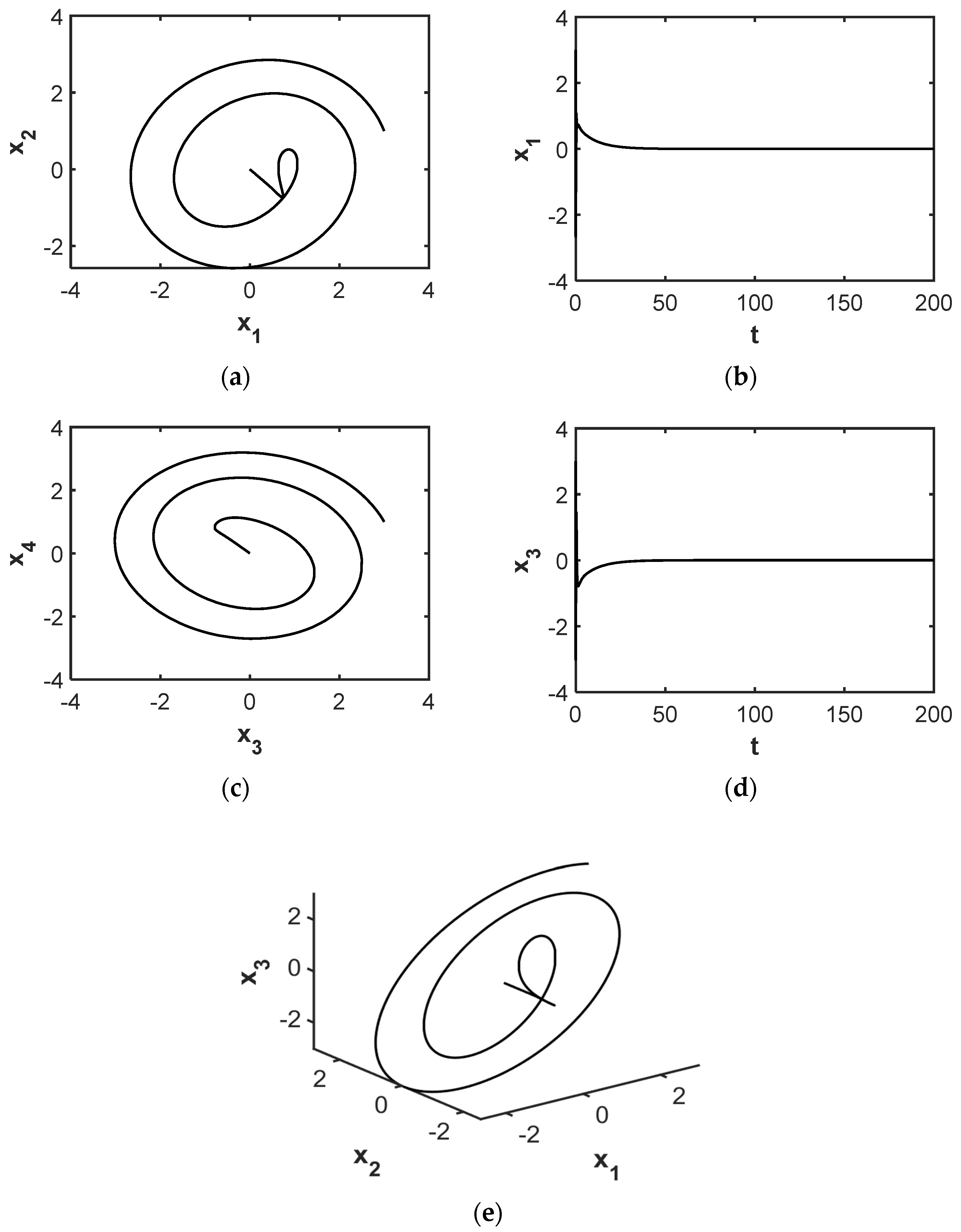
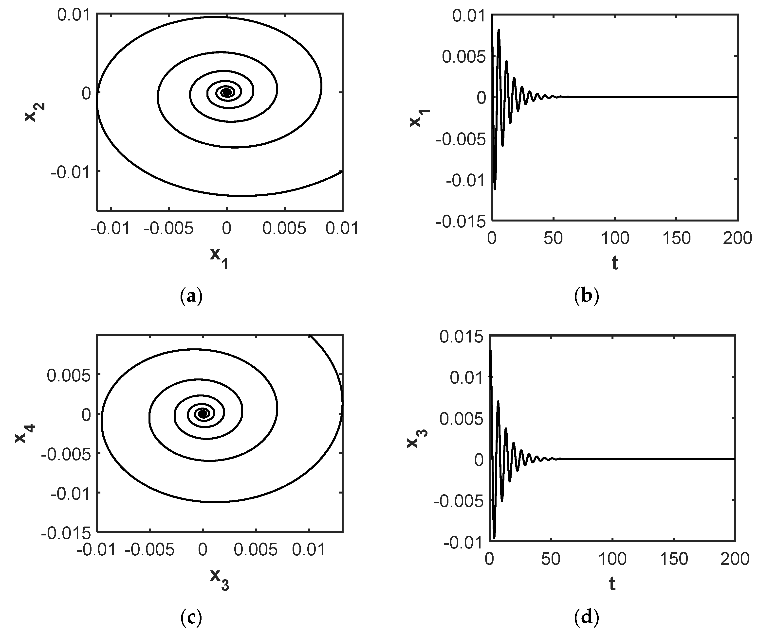
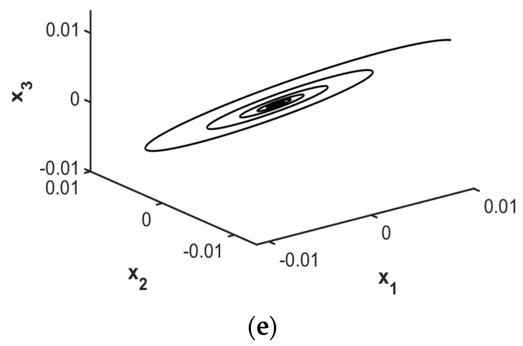
3.1. Case of Double Zero and Two Negative Eigenvalues

Taking parameters of the system (2) as ${\mu }_1={\mu }_2={\mu }_3={\mu }_4=1,{\mathsf{\Omega }}_0=1,{\sigma }_1=2,{\sigma }_2=-2,{\alpha }_1=2,{\alpha }_2={\alpha }_3=0,{\beta }_1=-2,{\beta }_2={\beta }_3=0$, which implies that $b_1=b_2=4,b_3=b_4=0$ and the Jacobi matrix (3) has the eigenvalues ${\lambda }_{1,2}=0,{\lambda }_{3,4}=-2$.

Consider the parameters ${\mu }_1$ and ${\mu }_3$ as perturbation parameters. Using the parameter transformations ${\mu }_1=1+{\delta }_1,{\mu }_3=1+{\delta }_2$ and the state variable transformations:

$$\left[\begin{array}{c}{x}_1\\ x_2\\ x_3\\ x_4\end{array}\right]=\left[\begin{array}{cccc}-3& -2& -1& -2\\ 2& 1& 2& 3\\ 1& 0& 1& 0\\ 0& 1& 0& 1\end{array}\right]\left[\begin{array}{c}{z}_1\\ z_2\\ z_3\\ z_4\end{array}\right].$$

(6)

yields

$${\dot{z}}_1=\left(\frac{1}{2}{\delta }_2-\frac{3}{2}{\delta }_1\right)z_1+\left({\delta }_2-{\delta }_1\right)z_2+\frac{1}{2}\left({\delta }_2-{\delta }_1\right)z_3+\left({\delta }_2-{\delta }_1\right)z_4+N{g}_1^2$$

(7a)

$${\dot{z}}_2=\left({\delta }_1-{\delta }_2\right)z_1+\left(\frac{1}{2}{\delta }_1-\frac{3}{2}{\delta }_2\right)z_2+\left({\delta }_1-{\delta }_2\right)z_3+\frac{3}{2}\left({\delta }_1-{\delta }_2\right)z_4+N{g}_2^2$$

(7b)

$${\dot{z}}_3=\frac{3}{2}\left({\delta }_1-{\delta }_2\right)z_1+\left({\delta }_1-{\delta }_2\right)z_2+\left(\frac{1}{2}{\delta }_1-\frac{3}{2}{\delta }_2-2\right)z_3+\left({\delta }_1-{\delta }_2\right)z_4+N{g}_3^2$$

(7c)

$${\dot{z}}_4=\left({\delta }_2-{\delta }_1\right)z_1+\frac{1}{2}\left({\delta }_2-{\delta }_1\right)z_2+\left({\delta }_2-{\delta }_1\right)z_3+\left(\frac{1}{2}{\delta }_2-\frac{3}{2}{\delta }_1-2\right)z_4+N{g}_4^2$$

(7d)

where the nonlinear terms $N{g}_i^2\left(i=1,2,3,4\right)$ are omitted since they are not crucial in the following discussion.

Computing the Jacobi matrix at equilibrium point $E=\left(0,0,0,0\right)$, we get

$$J_{\left(z_i=0\right)}=\left[\begin{array}{cccc}0& 0& 0& 0\\ 0& 0& 0& 0\\ 0& 0& -2& 0\\ 0& 0& 0& -2\end{array}\right].$$

(8)

Based on the center manifold theory, we can see that the local dynamic behaviors of the symmetric system (2) are determined by critical variables $z_1$ and $z_2$. The bifurcation solutions for the noncritical variables $z_3$ and $z_4$ can be obtained from (7c) and (7d) as follows,

$$z_3=\frac{3}{4}\left({\delta }_1-{\delta }_2\right)z_1+\frac{1}{2}\left({\delta }_1-{\delta }_2\right)z_2+N{g}_3^3,$$

(9a)

$$z_4=\frac{1}{2}\left({\delta }_2-{\delta }_1\right)z_1+\frac{1}{4}\left({\delta }_2-{\delta }_1\right)z_2+N{g}_4^3,$$

(9b)

where the nonlinear terms $N{g}_i^3\left(i=3,4\right)$ are omitted. We need only study the equations (10), to investigate the stability and bifurcation behaviors of the system (9) near-equilibrium point.

$${\dot{z}}_1=\left(-\frac{3}{2}{\delta }_1+\frac{1}{2}{\delta }_2+\frac{1}{8}{\delta }_1^2+\frac{1}{8}{\delta }_2^2-\frac{1}{4}{\delta }_1{\delta }_2\right)z_1+\left({\delta }_2-{\delta }_1\right)z_2+N{g}_1^3,$$

(10a)

$${\dot{z}}_2=\left({\delta }_1-{\delta }_2\right)z_1+\left(\frac{1}{2}{\delta }_1-\frac{3}{2}{\delta }_2+\frac{1}{8}{\delta }_1^2+\frac{1}{8}{\delta }_2^2-\frac{1}{4}{\delta }_1{\delta }_2\right)z_2+N{g}_2^3,$$

(10b)

where $N{g}_i^3\left(i=1,2\right)$ are also omitted.

The stability conditions of the equilibrium point $\left(z_1,z_2\right)=\left(0,0\right)$ are determined by the following Jacobi matrix,

$$J=\left[\begin{array}{cc}-\frac{3}{2}{\delta }_1+\frac{1}{2}{\delta }_2+\frac{1}{8}{\delta }_1^2+\frac{1}{8}{\delta }_2^2-\frac{1}{4}{\delta }_1{\delta }_2& {\delta }_2-{\delta }_1\\ {\delta }_1-{\delta }_2& \frac{1}{2}{\delta }_1-\frac{3}{2}{\delta }_2+\frac{1}{8}{\delta }_1^2+\frac{1}{8}{\delta }_2^2-\frac{1}{4}{\delta }_1{\delta }_2\end{array}\right],$$

(11)

The characteristic polynomial is

$$f\left(\lambda \right)={\lambda }^2+({\delta }_1+{\delta }_2-\frac{1}{4}{\left({\delta }_1-{\delta }_2\right)}^2)\lambda +{[\frac{1}{8}{\left({\delta }_1-{\delta }_2\right)}^2-\frac{1}{2}\left({\delta }_1+{\delta }_2\right)]}^2,$$

(12)

So the stability conditions for the equilibrium point $\left(z_1,z_2\right)=\left(0,0\right)$ are:

$${\delta }_1+{\delta }_2-\frac{1}{4}{\left({\delta }_1-{\delta }_2\right)}^2>0,{[\frac{1}{8}{\left({\delta }_1-{\delta }_2\right)}^2-\frac{1}{2}\left({\delta }_1+{\delta }_2\right)]}^2>0.$$

(13)

As we all know, ${[\frac{1}{8}{\left({\delta }_1-{\delta }_2\right)}^2-\frac{1}{2}\left({\delta }_1+{\delta }_2\right)]}^2>0$ is satisfied unless $\left({\delta }_1,{\delta }_2\right)=0$. Thus, the initial equilibrium solution is stable if ${\delta }_1+{\delta }_2-\frac{1}{4}{\left({\delta }_1-{\delta }_2\right)}^2>0$. Therefore, the transition curve $L_1$ is derived,

$$L_1:{\delta }_1+{\delta }_2-\frac{1}{4}{\left({\delta }_1-{\delta }_2\right)}^2=0.$$

(14)

The transition curve is shown in Figure 2. When the point $\left({\delta }_1,{\delta }_2\right)$ lies in the region I in Figure 2, the initial equilibrium solution is stable. In addition, the initial equilibrium solution is unstable when the point $\left({\delta }_1,{\delta }_2\right)$ lies in the region II.

Figure 2. Transition curves for the case of double zero and two negative eigenvalues.

Since the study here is focused on the local dynamic behaviors in the vicinity of a critical point, the parameter values $\left({\delta }_1,{\delta }_2\right)$ should be chosen near the point $\left({\delta }_1,{\delta }_2\right)=\left(0,0\right)$. According to the above criterion, choosing the parameter values $\left({\delta }_1,{\delta }_2\right)$ from the stable region for the initial equilibrium solution, such as $\left({\delta }_1,{\delta }_2\right)=\left(0.1,0.1\right)$, the numerical solution starting from $\left(x_1,x_2,x_3,x_4\right)=\left(3,1,3,1\right)$ converges to the origin, implying the initial equilibrium solution is stable, and the behaviors are shown in Figure 3.

Figure 3. Trajectory projection starting from $\left(x_1,x_2,x_3,x_4\right)=\left(3,1,3,1\right)$ converges to E.S. when $\left({\delta }_1,{\delta }_2\right)=\left(0.1,0.1\right)$. Diagrams (a,c) are, respectively, the trajectory projection converging to the origin on the planes $\left(x_1, x_2\right)$ and $\left(x_3, x_4\right)$. Diagrams (b,d) are the wave forms on the planes $\left(t, x_1\right)$ and $\left(t, x_3\right)$, and diagram (e) represents the trajectory projection converging to the origin in the space $\left(x_1,x_2,x_3\right)$.

3.2. Case of a Simple Zero and a Pair of Pure Imaginary Eigenvalu3

Taking parameters as ${\mu }_1=1,{\mu }_2={\mu }_3={\mu }_4=0,{\mathsf{\Omega }}_0=1,{\sigma }_1={\sigma }_2=1,{\alpha }_1=\sqrt{2},{\alpha }_2=1,{\alpha }_3={\beta }_1={\beta }_2={\beta }_3=0$, which implies that $b_1=b_3=2,b_2=1,b_4=0$ and the Jacobi matrix (5) has the eigenvalues ${\lambda }_1=0,{\lambda }_{2,3}=\pm i,{\lambda }_4=-2$.

We consider parameters ${\mu }_1$ and ${\mu }_3$ as perturbation parameters. Using the parameter transformations ${\mu }_1=1+{\delta }_1,{\mu }_3={\delta }_2$ and the state variable transformations:

$$\left[\begin{array}{c}{x}_1\\ x_2\\ x_3\\ x_4\end{array}\right]=\left[\begin{array}{cccc}-1-\sqrt{2}& \frac{2\sqrt{2}+2}{5}& \frac{-\sqrt{2}-1}{5}& 1-\sqrt{2}\\ 1& \frac{\sqrt{2}-1}{5}& \frac{2\sqrt{2}-2}{5}& 1\\ 0& 1& 0& 0\\ 0& 0& 1& 0\end{array}\right]\left[\begin{array}{c}{z}_1\\ z_2\\ z_3\\ z_4\end{array}\right].$$

(15)

into (3) yields

$${\dot{z}}_1=-{\delta }_1{z}_1+\frac{1}{2}\left({\delta }_1-{\delta }_2\right)z_2+\frac{\sqrt{2}-1}{2}\left({\delta }_2-{\delta }_1\right)z_3+N{g}_1^4,$$

(16a)

$${\dot{z}}_2=-{\delta }_2{z}_2+z_3+N{g}_2^4,$$

(16b)

$${\dot{z}}_3=-z_2-{\delta }_2{z}_3+N{g}_3^4,$$

(16c)

$${\dot{z}}_4=\frac{2\sqrt{2}+3}{10}\left({\delta }_2-{\delta }_1\right)z_2+\frac{\sqrt{2}-1}{10}\left({\delta }_1-{\delta }_2\right)z_3+\left(-2-{\delta }_1\right)z_4+N{g}_4^4,$$

(16d)

where $N{g}_i^4\left(i=1,2,3,4\right)$ denote the nonlinear functions and they are omitted since they are not significant in the following analysis.

The Jacobi matrix of system (16) evaluated at the initial equilibrium solution $\left(x_1,x_2,x_3,x_4\right)=\left(0,0,0,0\right)$ at critical point ${\delta }_1={\delta }_2=0$ is in the following canonical form,

$$J_{\left(z_i=0\right)}=\left[\begin{array}{cccc}0& 0& 0& 0\\ 0& 0& 1& 0\\ 0& -1& 0& 0\\ 0& 0& 0& -2\end{array}\right].$$

(17)

Based on the center manifold theory, we know that the local dynamic behaviors of the system (16) are determined by critical variables $z_1$, $z_2$ and $z_3$. Introducing a near identity nonlinear transform $z_i=y_i+g_i\left(y_j\right)$ (which are omitted since they are not significant in the following analysis) and a cylindrical coordinate transform $z_1=y,z_2=rcos\theta ,z_3=rsin\theta ,z_4=z_4$, we get the normal form of system (16) as follows,

$$\dot{y}=y(-{\delta }_1+(\frac{14}{5}+\frac{8}{5}\sqrt{2})r^2+(4+2\sqrt{2})y^2),$$

(18a)

$$\dot{r}=r(-{\delta }_2+(-\frac{8}{25}-\frac{4}{25}\sqrt{2})r^2+(-\frac{6}{5}-\frac{6}{5}\sqrt{2})y^2),$$

(18b)

and

$$\dot{\theta }=-1+\left(\frac{46}{25}+\frac{28}{25}\sqrt{2}\right)r^2+(\frac{42}{5}+\frac{32}{5}\sqrt{2})y^2.$$

(19)

We now discuss steady-state solutions and their stability basis of (20). It is worth noting that the characteristics of the steady-state solutions can be validated by calculating the Jacobian of the system (18). The discussion can be divided into four categories, and the Jacobi matrix of (20) is as follows:

$$J=\left[\begin{array}{cc}-{\delta }_1+\left(\frac{14}{5}+\frac{8}{5}\sqrt{2}\right)r^2+6\left(2+\sqrt{2}\right)y^2& \left(\frac{28}{5}+\frac{16}{5}\sqrt{2}\right)yr\\ \left(-\frac{12}{5}-\frac{12}{5}\sqrt{2}\right)yr& -{\delta }_2-\frac{12}{25}\left(2+\sqrt{2}\right)r^2-\frac{6}{5}\left(1+\sqrt{2}\right)y^2\end{array}\right].$$

(20)

(I) The initial equilibrium solution (E.S.)

$$y=r=0.$$

(21)

The Jacobi matrix of system (18) is as follows,

$$J=\left[\begin{array}{cc}-{\delta }_1& 0\\ 0& -{\delta }_2\end{array}\right].$$

(22)

Thus, the stability conditions for the E.S. at the initial equilibrium solution are ${\delta }_1>0$ and ${\delta }_2>0$, or the initial E.S. is unstable. So, the transition curves which define the stability boundaries of the E.S. are $L_2:{\delta }_2=0({\delta }_1>0)$ and $L_2:{\delta }_2=0({\delta }_1>0)$.

(II) The static bifurcation solution (S.B.):

$$y^2=\frac{2-\sqrt{2}}{4}{\delta }_1,r=0.$$

(23)

It is obvious that there exists an S.B. solution when ${\delta }_1>0$. The Jacobi matrix of (20) is as follows

$$J=\left[\begin{array}{cc}2{\delta }_1& 0\\ 0& -\frac{3\sqrt{2}}{10}{\delta }_1-{\delta }_2\end{array}\right].$$

(24)

Thus, the stability conditions for the S.B. solution are ${\delta }_1<0$ and $-\frac{3\sqrt{2}}{10}{\delta }_1-{\delta }_2<0$. So the S.B. solution is unstable when ${\delta }_1>0$. In addition, we can get a transition curve $L_4:{\delta }_2+\frac{3\sqrt{2}}{10}{\delta }_1=0({\delta }_1<0)$.

(III) The incipient Hopf bifurcation solution (H.B.(I)):

$$y=0,r^2=-\frac{25}{8+4\sqrt{2}}{\delta }_2.$$

(25)

The incipient H.B. solution exists when ${\delta }_2<0$. The Jacobi matrix of (20) is as follows,

$$J=\left[\begin{array}{cc}-{\delta }_1-\frac{5\sqrt{2}+30}{4}{\delta }_2& 0\\ 0& 2{\delta }_2\end{array}\right].$$

(26)

Thus, the stability conditions for the H.B.(I) solution are $-{\delta }_1-\frac{5\sqrt{2}+30}{4}{\delta }_2<0$ and ${\delta }_2<0$. Therefore, the transition curves which define the stability boundaries of the H.B.(I) solution are $L_2:{\delta }_2=0({\delta }_1>0)$ and $L_5:{\delta }_1+\frac{5\sqrt{2}+30}{4}{\delta }_2=0({\delta }_2<0)$.

(IV) The secondary solution H.B.(II):

$$y^2=\frac{-2\left(6-\sqrt{2}\right){\delta }_1-85{\delta }_2}{86\sqrt{2}+62},r^2=\frac{75\sqrt{2}{\delta }_1+50{\delta }_2}{32+34\sqrt{2}}.$$

(27)

The secondary H.B. solution exists when ${\delta }_1+\frac{5\sqrt{2}+30}{4}{\delta }_2<0,3{\delta }_1+\sqrt{2}{\delta }_2>0$. The Jacobi matrix of (20) is as follows,

$$J=\left[\begin{array}{cc}4\left(2+\sqrt{2}\right)y^2& \frac{4\left(7+4\sqrt{2}\right)}{5}yr\\ -\frac{12\left(1+\sqrt{2}\right)}{5}yr& -\frac{8\left(2+\sqrt{2}\right)}{25}{r}^2\end{array}\right].$$

(28)

Thus, the stability conditions for the H.B.(II) solution are $Tr=\frac{-2\left(358\sqrt{2}+640\right){\delta }_1-2\left(1617\sqrt{2}+1484\right){\delta }_2}{236\sqrt{2}+743}<0$ and $Det=\frac{16\left(25\sqrt{2}+33\right)}{25}{y}^2{r}^2>0$. When the H.B.(II) solution exists, the condition $Det=\frac{16\left(25\sqrt{2}+33\right)}{25}{y}^2{r}^2>0$ must be met. So ${\delta }_1+\frac{5\sqrt{2}+30}{4}{\delta }_2<0,3{\delta }_1+\sqrt{2}{\delta }_2>0,\left(358\sqrt{2}+640\right){\delta }_1+\left(1617\sqrt{2}+1484\right){\delta }_2>0$, H.B.(II) solution is stable and exists. Therefore, the transition curves which define the stability boundaries of the H.B.(II) solution are $L_5:{\delta }_1+\frac{5\sqrt{2}+30}{4}{\delta }_2=0({\delta }_2<0)$ and $L_6:\left(358\sqrt{2}+640\right){\delta }_1+\left(1617\sqrt{2}+1484\right){\delta }_2=0({\delta }_1+\frac{5\sqrt{2}+30}{4}{\delta }_2<0)$.

As a result, we can conclude: The incipient H.B. solution first bifurcates from the initial E.S. along the transition curve $L_2$; when the parameters cross the transition curve $L_5$, the incipient H.B. solution loses its stability and bifurcates into a family of limit cycle (H.B.(II)); and finally, the H.B.(II) solution loses its stability and bifurcates into a two-dimensional torus along the transition curve $L_6$. The transition curves are illustrated in Figure 4.

Figure 4. Transition curves for the case of a simple zero and a pair of pure imaginary eigenvalues.

Now, we select different parameter values in different areas of Figure 4 to prove the analysis results. First, choosing $\left({\delta }_1,{\delta }_2\right)=\left(0.1,0.1\right)$ which is located in the stable region for the E.S., the trajectory starting from $\left(x_1,x_2,x_3,x_4\right)=\left(0.1,0.1,0.1,0.1\right)$ converges to the origin shown in Figure 5. Second, choosing $\left({\delta }_1,{\delta }_2\right)=\left(0.1,-0.001\right)$ which is located in the stable region for H.B.(I) solution, the trajectory starting from $\left(x_1,x_2,x_3,x_4\right)=\left(0.1,0.1,0.1,0.1\right)$ yields a stable limit cycle shown in Figure 6. Finally, choosing $\left({\delta }_1,{\delta }_2\right)=\left(0.1,-0.011\right)$ which is located in the stable region for H.B.(II) solution, the trajectory starting from $\left(x_1,x_2,x_3,x_4\right)=\left(0.1,0.1,0.1,0.1\right)$ yields a stable limit cycle shown in Figure 7.

Figure 5. Trajectory projection starting from $\left(x_1,x_2,x_3,x_4\right)=\left(0.1,0.1,0.1,0.1\right)$ converges to the E.S. when $\left({\delta }_1,{\delta }_2\right)=\left(0.1,0.1\right)$. Diagrams (a,c) are, respectively, the trajectory projection converging to E.S. on the planes $\left(x_1, x_2\right)$ and $\left(x_3, x_4\right)$. Diagrams (b,d) are the wave forms on the planes $\left(t, x_1\right)$ and $\left(t, x_3\right)$, and diagram (e) shows the trajectory projection converging to E.S. in the space $\left(x_1,x_2,x_3\right)$.

Figure 6. Trajectory projection starting from $\left(x_1,x_2,x_3,x_4\right)=\left(0.1,0.1,0.1,0.1\right)$ yields a stable limit cycle when $\left({\delta }_1,{\delta }_2\right)=\left(0.1,-0.001\right)$. Diagrams (a,c) are, respectively, the trajectory projection converging to H.B.(I) on the planes $\left(x_1, x_2\right)$ and $\left(x_3, x_4\right)$. Diagrams (b,d) are the wave forms on the planes $\left(t, x_1\right)$ and $\left(t, x_3\right)$, and diagram (e) shows the trajectory projection converging to H.B.(I) in the space $\left(x_1,x_2,x_3\right)$.

Figure 7. Trajectory projection starting from $\left(x_1,x_2,x_3,x_4\right)=\left(0.1,0.1,0.1,0.1\right)$ yields a stable limit cycle when $\left({\delta }_1,{\delta }_2\right)=\left(0.1,-0.011\right)$. Diagrams (a,c) are, respectively, the trajectory projection converging to H.B.(II) on the planes $\left(x_1,x_2\right)$ and $\left(x_3,x_4\right)$. Diagrams (b,d) are the wave forms on the planes $\left(t,x_1\right)$ and $\left(t,x_3\right)$, and diagram (e) indicates the trajectory projection converging to H.B.( II) in the space $\left(x_1,x_2,x_3\right)$.

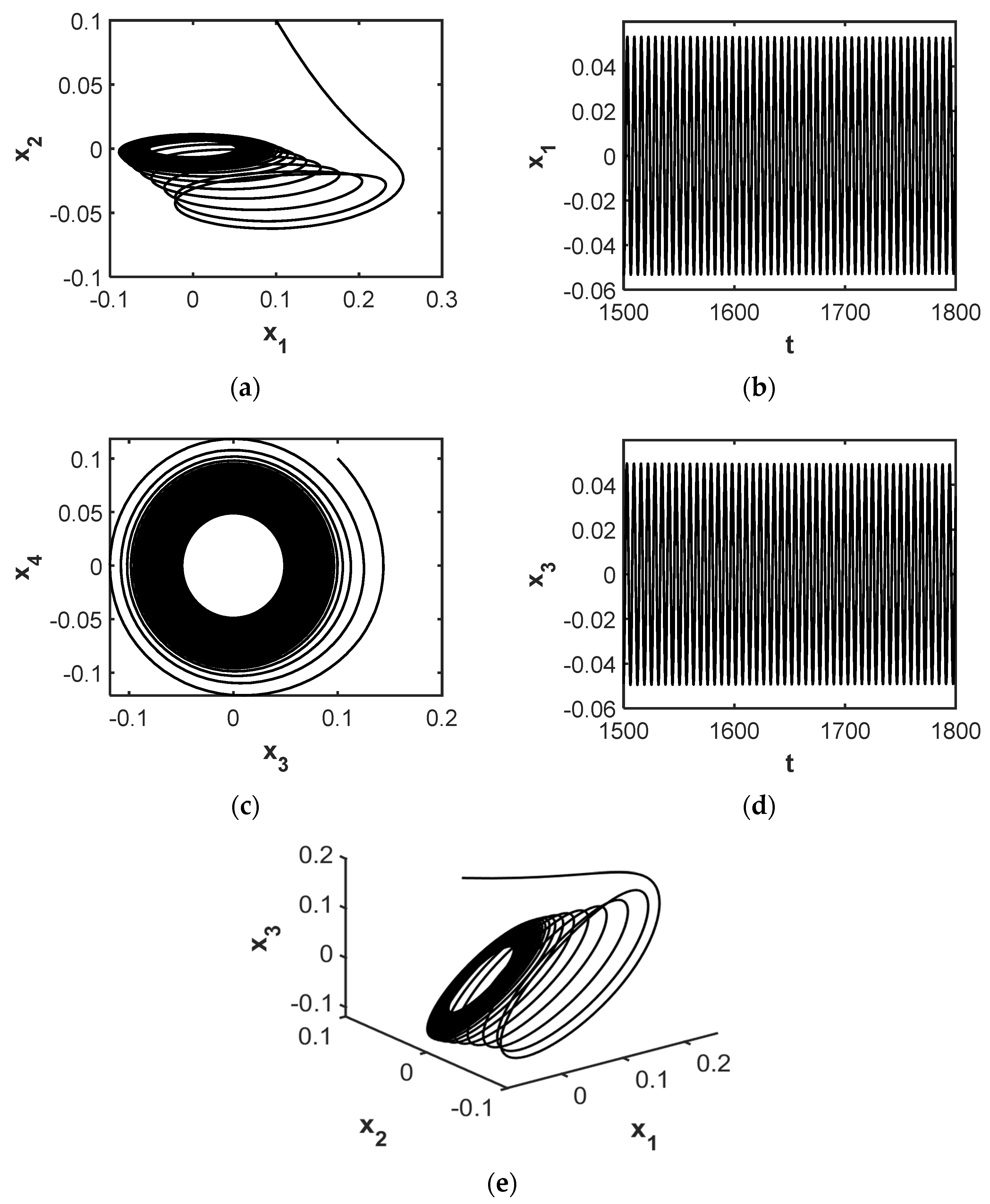
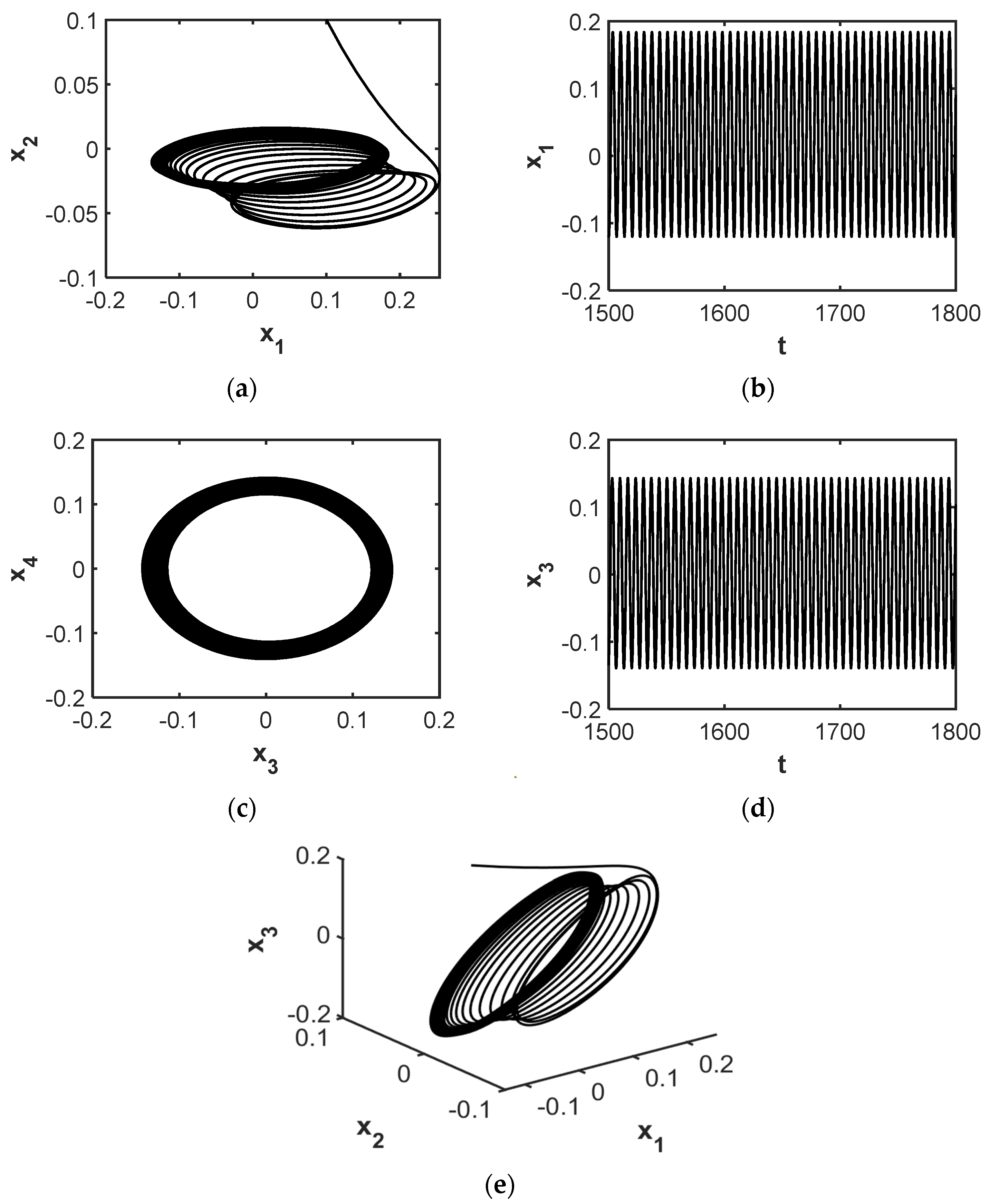
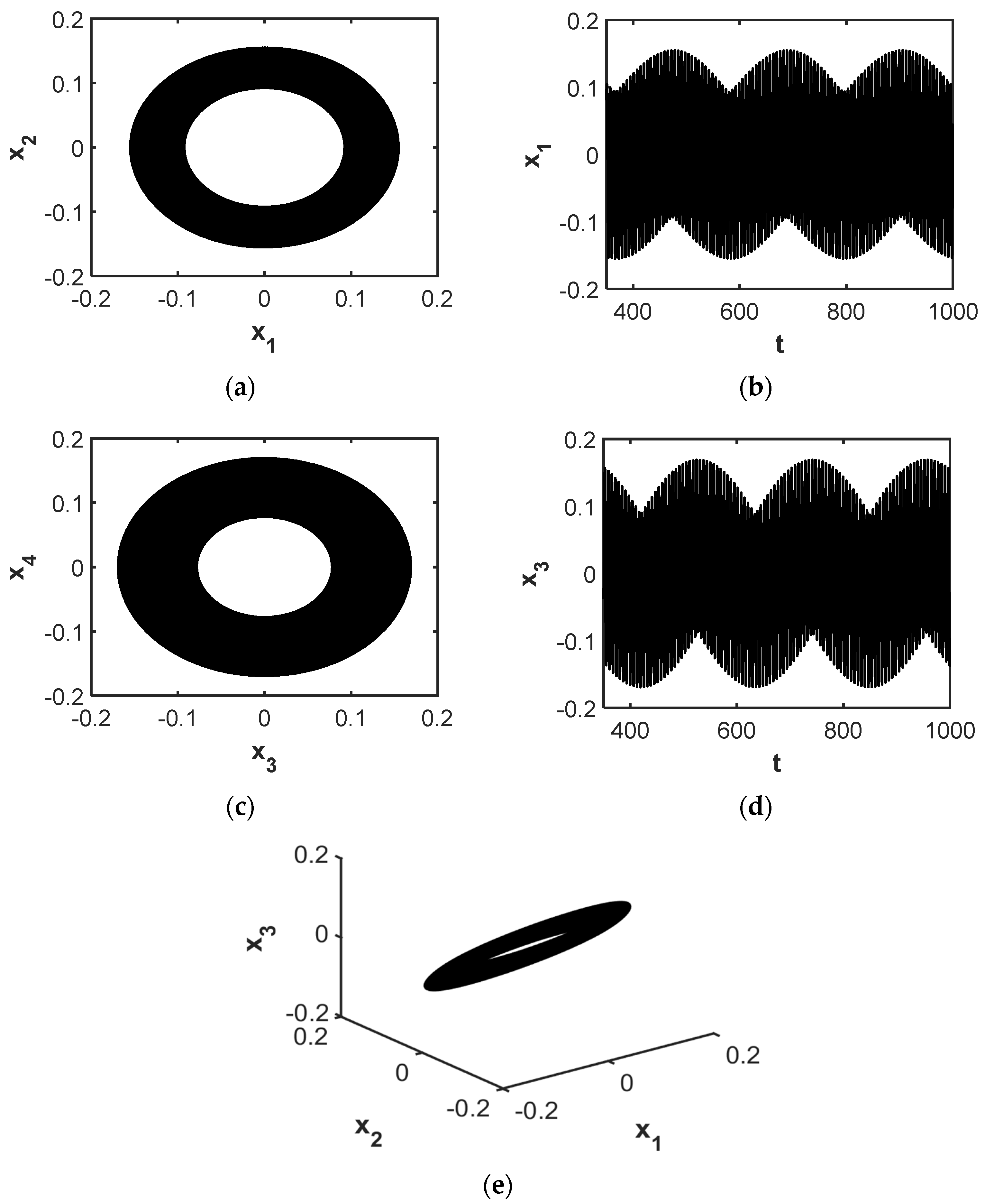
3.3. Case of Two Different Pairs of Pure Imaginary Eigenvalues

Taking parameters as ${\mu }_1={\mu }_3=0,{\mu }_2=2,{\mu }_4=3,{\mathsf{\Omega }}_0=1,{\sigma }_1=-1,{\sigma }_2=4,{\alpha }_1={\alpha }_2={\alpha }_3={\beta }_1={\beta }_2={\beta }_3=0,$ which implies that $b_1=b_3=0,b_2=5,b_4=4$ and the Jacobi matrix (5) has the eigenvalues ${\lambda }_{1,2}=\pm i,{\lambda }_{3,4}=\pm 2i$.

We consider parameters ${\mu }_1$ and ${\mu }_3$ as perturbation parameters. Using the parameter transformations ${\mu }_1={\delta }_1,{\mu }_3={\delta }_2$ and the state variable transformations:

$$\left[\begin{array}{c}{x}_1\\ x_2\\ x_3\\ x_4\end{array}\right]=\left[\begin{array}{cccc}0& 1& 0& \frac{2}{3}\\ -1& 0& -\frac{2}{3}& 0\\ 1& 0& 1& 0\\ 0& 1& 0& 1\end{array}\right]\left[\begin{array}{c}{z}_1\\ z_2\\ z_3\\ z_4\end{array}\right].$$

(29)

into (2) yields

$${\dot{z}}_1=\left(-3{\delta }_1+2{\delta }_2\right)z_1+z_2+\left(-2{\delta }_1+2{\delta }_2\right)z_3+N{g}_1^5,$$

(30a)

$${\dot{z}}_2=-z_1+\left(-3{\delta }_1+2{\delta }_2\right)z_2+\left(-2{\delta }_1+2{\delta }_2\right)z_4+N{g}_2^5,$$

(30b)

$${\dot{z}}_3=\left(3{\delta }_1-3{\delta }_2\right)z_1+\left(2{\delta }_1-3{\delta }_2\right)z_3+2z_4+N{g}_3^5,$$

(30c)

$${\dot{z}}_4=\left(3{\delta }_1-3{\delta }_2\right)z_2-2z_3+\left(2{\delta }_1-3{\delta }_2\right)z_4+N{g}_4^5,$$

(30d)

where $N{g}_i^5\left(i=1,2,3,4\right)$ denote the nonlinear functions and they are omitted since they are not significant in the following analysis.

The Jacobi matrix of symmetric system (30) evaluated at the initial E.S. $\left(x_1,x_2,x_3,x_4\right)=\left(0,0,0,0\right)$ at critical point ${\delta }_1={\delta }_2=0$ is in the following canonical form,

$$J_{\left(z_i=0\right)}=\left[\begin{array}{cccc}0& 1& 0& 0\\ -1& 0& 0& 0\\ 0& 0& 0& 2\\ 0& 0& -2& 0\end{array}\right].$$

(31)

We use a near identity nonlinear transform $z_i=y_i+g_i\left(y_j\right)$ (which are omitted since they are not significant in the following analysis) and a polar coordinate transform $y_1=r_{1}cos{\theta }_1,y_2=r_{1}sin{\theta }_1,y_3=r_{2}cos{\theta }_2,y_4=r_{2}sin{\theta }_2$, we get the normal form of symmetric system (30) as follows,

$$\dot{r_1}=r_1\left(-3{\delta }_1+2{\delta }_2-5r_1{}^2-\frac{70}{9}{r}_2{}^2\right),$$

(32a)

$$\dot{r_2}=r_2\left(2{\delta }_1-3{\delta }_2+10r_1{}^2+\frac{35}{9}{r}_2{}^2\right),$$

(32b)

and

$$\dot{{\theta }_1}=1+r_1{}^2+\frac{1}{9}{r}_2{}^2,$$

(33a)

$$\dot{{\theta }_2}=2+4r_1{}^2+\frac{19}{9}{r}_2{}^2.$$

(33b)

We now discuss the bifurcation and stability behaviors of the symmetric system (30). Note that the characters of the steady-state solutions can be verified by evaluating the Jacobian of the system (32). The discussion can fall into four categories and the Jacobi matrix of (34) is as follows,

$$J=\left[\begin{array}{cc}-3{\delta }_1+2{\delta }_2-15r_1{}^2-\frac{70}{9}{r}_2{}^2& -\frac{140}{9}{r}_1{r}_2\\ 20r_1{r}_2& 2{\delta }_1-3{\delta }_2+10r_1{}^2+\frac{35}{3}{r}_2{}^2\end{array}\right].$$

(34)

(I) The initial E.S.:

$$r_1=r_2=0.$$

(35)

The Jacobi matrix of (34) is as follows,

$$J=\left[\begin{array}{cc}-3{\delta }_1+2{\delta }_2& 0\\ 0& 2{\delta }_1-3{\delta }_2\end{array}\right].$$

(36)

Thus, the stability conditions for the E.S. at the initial equilibrium solution are $3{\delta }_1-2{\delta }_2>0$ and $2{\delta }_1-3{\delta }_2<0$, or the initial E.S. is unstable. So the transition curves which define the stability boundaries of the E.S. are $L_7:3{\delta }_1-2{\delta }_2=0(2{\delta }_1-3{\delta }_2<0)$ and $L_8:2{\delta }_1-3{\delta }_2=0(3{\delta }_1-2{\delta }_2>0)$.

(II) The incipient H.B. solution (I):

$$r_1{}^2=\frac{-3{\delta }_1+2{\delta }_2}{5},r_2=0.$$

(37)

It is obvious that there exists H.B.(I) solution when $3{\delta }_1-2{\delta }_2<0$. The Jacobi matrix of (34) is as follows,

$$J=\left[\begin{array}{cc}2\left(3{\delta }_1-2{\delta }_2\right)& 0\\ 0& -4{\delta }_1+{\delta }_2\end{array}\right].$$

(38)

Thus, the stability conditions for the H.B.(I) solution are $3{\delta }_1-2{\delta }_2<0$ and $4{\delta }_1-{\delta }_2>0$. So we can get two transition curves $L_7:3{\delta }_1-2{\delta }_2=0(2{\delta }_1-3{\delta }_2<0)$ and $L_9:4{\delta }_1-{\delta }_2=0(3{\delta }_1-2{\delta }_2<0)$.

(III) The secondary H.B. solution (II):

$$r_1=0,r_2{}^2=-\frac{9}{35}\left(2{\delta }_1-3{\delta }_2\right).$$

(39)

H.B.(II) solution exists when $2{\delta }_1-3{\delta }_2<0$. The Jacobi matrix of (34) is as follows,

$$J=\left[\begin{array}{cc}{\delta }_1-4{\delta }_2& 0\\ 0& 2\left(3{\delta }_2-2{\delta }_1\right)\end{array}\right].$$

(40)

Thus, the stability conditions for the H.B.(II) solution are ${\delta }_1-4{\delta }_2<0$ and $2{\delta }_1-3{\delta }_2>0$. So, the H.B.(II) solution is unstable when $2{\delta }_1-3{\delta }_2<0$. Therefore, the transition curves which define the stability boundaries of the H.B.(II) solution are $L_8:2{\delta }_1-3{\delta }_2=0(3{\delta }_1-2{\delta }_2>0)$ and $L_{10}:{\delta }_1-4{\delta }_2=0(2{\delta }_1-3{\delta }_2>0)$.

(IV) Quasi-periodic solution (2-D torus):

$$r_1{}^2=\frac{1}{15}\left(4{\delta }_2-{\delta }_1\right),r_2{}^2=\frac{3}{35}\left(-4{\delta }_1+{\delta }_2\right).$$

(41)

The Quasi-periodic solution exists when ${\delta }_1-4{\delta }_2<0,4{\delta }_1-{\delta }_2<0$. The Jacobi matrix of (34) is as follows,

$$J=\left[\begin{array}{cc}-10r_1{}^2& -\frac{140}{9}{r}_1{r}_2\\ 20r_1{r}_2& \frac{70}{9}{r}_2{}^2\end{array}\right].$$

(42)

Thus, the stability conditions for the Quasi-periodic solution are $Tr=-2\left({\delta }_1+{\delta }_2\right)<0$ and $Det=\frac{700}{3}{r}_1{}^2{r}_2{}^2>0$. When the Quasi-periodic solution exists, the condition $Det=\frac{700}{3}{r}_1{}^2{r}_2{}^2>0$ must be met. So, when ${\delta }_1-4{\delta }_2<0, 4{\delta }_1-{\delta }_2<0, {\delta }_1+{\delta }_2>0$, Quasi-periodic solution is stable and exists. Therefore, the transition curves which define the stability boundaries of the Quasi-periodic solution are $L_9:4{\delta }_1-{\delta }_2=0(3{\delta }_1-2{\delta }_2<0)$ and $L_{11}:{\delta }_1+{\delta }_2=0 (4{\delta }_1-{\delta }_2<0)$.

As a result, we can draw the following conclusions: The initial E.S. occurs first when the parameters are in the region between $L_7$ and $L_8$; then, the incipient H.B. solution bifurcates from the initial E.S. along the transition curve $L_7$; and finally, when the parameters pass-through $L_9$ from $L_7$, the incipient H.B. solution loses its stability and bifurcates into a two-dimensional torus along the transition curve $L_9$. The transition curves are illustrated in Figure 8.

Figure 8. Transition curves for the case of two different pairs of pure imaginary eigenvalues.

Now we select different parameter values in different areas of Figure 8 to prove the analysis results. First, choosing $\left({\delta }_1,{\delta }_2\right)=\left(0.1,0.1\right)$ which is located in the stable region for the E.S., the trajectory starting from $\left(x_1,x_2,x_3,x_4\right)=\left(0.01,-0.01,0.01,0.01\right)$ converges to the origin shown in Figure 9. Second, choosing $\left({\delta }_1,{\delta }_2\right)=\left(0.03,0.05\right)$ which is located in the stable region for H.B.(I) solution, the trajectory starting from $\left(x_1,x_2,x_3,x_4\right)=\left(0.001,-0.001,0.001,0.001\right)$ yields a stable limit cycle shown in Figure 10. Finally, choosing $\left({\delta }_1,{\delta }_2\right)=\left(0.01,0.06\right)$ which is located in the stable region for Quasi-periodic solution, the trajectory starting from $\left(x_1,x_2,x_3,x_4\right)=\left(0.1,-0.1,0.1,0.1\right)$ yields a stable 2-D torus shown in Figure 11.

Figure 9. Trajectory projection starting from $\left(x_1,x_2,x_3,x_4\right)=\left(0.01,-0.01,0.01,0.01\right)$ converges to the E.S. when $\left({\delta }_1,{\delta }_2\right)=\left(0.1,0.1\right)$. Diagrams (a,c) are, respectively, the trajectory projection converging to the origin on the planes $\left(x_1,x_2\right)$ and $\left(x_3,x_4\right)$. Diagrams (b,d) are the wave forms on the planes $\left(t,x_1\right)$ and $\left(t,x_3\right)$, and diagram (e) means the trajectory projection converging to the origin in the space $\left(x_1,x_2,x_3\right)$.

Figure 10. Trajectory projection starting from $\left(x_1,x_2,x_3,x_4\right)=\left(0.001,-0.001,0.001,0.001\right)$ yields a stable limit cycle when $\left({\delta }_1,{\delta }_2\right)=\left(0.03,0.05\right)$. Diagrams (a,c) are, respectively, the trajectory projection converging to H.B.(I) on the planes $\left(x_1,x_2\right)$ and $\left(x_3,x_4\right)$. Diagrams (b,d) are the wave forms on the planes $\left(t,x_1\right)$ and $\left(t,x_3\right)$, and diagram (e) indicates the trajectory projection converging to H.B.(I) in the space $\left(x_1,x_2,x_3\right)$.

Figure 11. Trajectory projection starting from $\left(x_1,x_2,x_3,x_4\right)=\left(0.1,-0.1,0.1,0.1\right)$ yields a stable 2-D torus when $\left({\delta }_1,{\delta }_2\right)=\left(0.01,0.06\right)$. Diagrams (a,c) are, respectively, the trajectory projection converging to 2-D torus on the planes $\left(x_1,x_2\right)$ and $\left(x_3,x_4\right)$. Diagrams (b,d) are the wave forms on the planes $\left(t,x_1\right)$ and $\left(t,x_3\right)$, and diagram (e) shows the trajectory projection converging to 2-D torus in the space $\left(x_1,x_2,x_3\right)$.

4. Conclusions

In this paper, the dynamic behavior of the bifurcation equations near the three critical points of the symmetric FGM rotating cantilever plate system in the case of the 1:1 internal resonance is studied. The three types of degenerate equilibrium points are analyzed using the central manifold theory, normal form theory, bifurcation theory, and stability theory, and the stability conditions and transition curves leading to S.B., H.B., and bifurcation of the two-dimensional torus are obtained. We use the fourth-order Runge–Kutta method to solve the numerical solution, and the results show that the numerical results are consistent with the analytical results.

From the above analysis, we can obtain that the calculation of the normal form of nonlinear system brings great convenience to simplify the engineering model and study the bifurcation and stability behaviors of the nonlinear dynamic system. As we all know, the nonlinear system may have different qualitative structures under different disturbance conditions, the type of singularity may change, and the qualitative structure and topology of the trajectory near the singularity will also be affected. In engineering, many special nonlinear dynamic behaviors, such as wing instability and automatic rotation, are closely related to bifurcation behavior. Therefore, it is necessary to use the bifurcation and stability theory to analyze and simulate the dynamic mechanism of the FGM plate.

References

- Miyamoto, Y.; Kaysser, W.A.; Rabin, B.H.; Kawasaki, A.; Ford, R.G. Functionally Graded Materials: Design, Processing and Applications; Springer Science and Business Media: Berlin/Heidelberg, Germany, 2013. [Google Scholar]
- Wang, Y.Q.; Zu, J.W. Nonlinear oscillations of sigmoid functionally graded material plates moving in longitudinal direction. Appl. Math. Mech. 2017, 38, 1533–1550. [Google Scholar] [CrossRef]
- Reddy, J.N. Analysis of functionally graded plates. Int. J. Numer. Methods Eng. 2000, 47, 663–684. [Google Scholar] [CrossRef]
- Guo, X.Y.; Zhang, B.; Cao, D.X.; Sun, L. Influence of nonlinear terms on dynamical behavior of graphene reinforced laminated composite plates. Appl. Math. Model. 2020, 78, 169–184. [Google Scholar] [CrossRef]
- Zhang, W.; Wu, Z.; Guo, X.Y. Nonlinear dynamics of rotating cantilever FGM rectangular plate with varying rotating speed. Sci. Technol. Rev. 2012, 30, 30–37. [Google Scholar]
- Li, Z.N.; Hao, Y.X.; Zhang, W.; Zhang, J.H. Nonlinear Transient Response of Functionally Graded Material Sandwich Doubly Curved Shallow Shell Using New Displacement Field. Acta Mech. Solida Sin. 2018, 31, 108–126. [Google Scholar] [CrossRef]
- Sitli, Y.; Mhada, K.; Bourihane, O.; Rhanim, H. Buckling and post-buckling analysis of a functionally graded material (FGM) plate by the asymptotic numerical method. Structure 2021, 31, 1031–1040. [Google Scholar] [CrossRef]
- Tao, C.; Dai, T. Analyses of thermal buckling and secondary instability of post-buckled S-FGM plates with porosities based on a meshfree method. Appl. Math. Model. 2021, 89, 268–284. [Google Scholar] [CrossRef]
- Zhang, X.H.; Chen, F.Q.; Zhang, H.L. Stability and local bifurcation analysis of functionally graded material plate under transversal and in-plane excitations. Appl. Math. Model. 2013, 37, 6639–6651. [Google Scholar] [CrossRef]
- Sharma, S.; Singh, F. Bifurcation and stability analysis of a cholera model with vaccination and saturated trearment. Chaos Solitons Fractals 2021, 146, 110912. [Google Scholar] [CrossRef]
- Tian, X.; Xu, R.; Lin, J. Mathematical analysis of a cholera infection model with vaccination strategy. Appl. Math. Comput. 2019, 361, 517–535. [Google Scholar] [CrossRef]
- Yu, P.; Huseyin, K. A perturbation analysis of interactive static and dynamic bifurcations. IEEE Trans. Autom. Control. 1988, 33, 28–41. [Google Scholar] [CrossRef]
- Yu, P.; Huseyin, K. On bifurcation into nonresonant quasi-periodic motions. Appl. Math. Model. 1988, 12, 189–201. [Google Scholar]
- Yu, P.; Huseyin, K. Bifurcations associated with a three-fold zero eigenvalue. Q. Appl. Math. 1988, 46, 193–216. [Google Scholar] [CrossRef]
- Yu, P.; Huseyin, K. Bifurcations associated with a double zero and a pair of pure imaginary eigenvalues. SIAM J. Appl. Math. 1988, 48, 229–261. [Google Scholar] [CrossRef][Green Version]
- Cai, T.Y.; Jin, H.L.; Yu, H.; Xie, X.P. On stability switches and bifurcation of the modified autonomous Van der Pol-Duffing equations via delayed state feedback control. Symmetry 2021, 13, 2336. [Google Scholar] [CrossRef]
- Yu, P. Analysis on double Hopf bifurcation using computer algebra with the aid of multiple scales. Nonlinear Dyn. 2002, 27, 19–53. [Google Scholar] [CrossRef]
- Gazor, M.; Mokhtari, F. Norm forms of Hopf-zero singularity. Int. J. Bifurc. Chaos 2008, 18, 2293–3408. [Google Scholar] [CrossRef]
- Yu, P. Symbolic computation of normal forms for resonant double Hopf bifurcations using a perturbation technique. J. Sound Vib. 2001, 247, 615–632. [Google Scholar] [CrossRef][Green Version]
- Xue, M.; Gou, J.T.; Xia, Y.B.; Bi, Q.S. Computation of the normal form as well as the unfolding of the vector field with zero-zero-Hopf bifurcation at the origin. Math. Comput. Simul. 2021, 190, 377–397. [Google Scholar] [CrossRef]
- Algaba, A.; Fuentes, N.; Gamero, E.; Garcia, C. Orbital normal forms for a class of three-dimensional systems with an application to Hopf-zero bifurcation analysis of Fitzhugh–Nagumo system. Appl. Math. Comput. 2020, 369, 124893. [Google Scholar] [CrossRef]
- Algaba, A.; Fuentes, N.; Gamero, E.; Garcia, C. On the integrability problem for the Hopf-zero singularity and its relation with the inverse Jacobi multiplier. Appl. Math. Comput. 2021, 405, 126241. [Google Scholar] [CrossRef]
- Kincaid, D.; Cheney, W. Numerical Analysis: Mathematics of Science Computing; American Mathematical Society: Providence, RI, USA, 2009. [Google Scholar]
- Huang, J.L.; Wang, T.; Zhu, W.D. An incremental harmonic balance method with two-scales for quasi-periodic responses of a Van der Pol-Mathieu equation. Int. J. Non-Linear Mech. 2021, 135, 103767. [Google Scholar] [CrossRef]
- Huang, J.L.; Zhou, W.J.; Zhu, W.D. Quasi-periodic motions of high-dimensional nonlinear models of a translating beam with a stationary load subsystem under harmonic boundary excitation. J. Sound Vib. 2019, 462, 114870. [Google Scholar] [CrossRef]
Publisher’s Note: MDPI stays neutral with regard to jurisdictional claims in published maps and institutional affiliations. |
© 2022 by the authors. Licensee MDPI, Basel, Switzerland. This article is an open access article distributed under the terms and conditions of the Creative Commons Attribution (CC BY) license (https://creativecommons.org/licenses/by/4.0/).