Decision Making of Software Release Time at Different Confidence Intervals with Ohba’s Inflection S-Shape Model

Abstract

Software developers need information for deciding the optimal time for software release with improved software reliability. However, it is not easy for them to decide when and how to release newly developed software to the market. For a decision, the reliability and test costs of the software need to be balanced carefully for avoiding unnecessary confusion and users’ complaints. To address this need, related research has been carried out to propose an appropriate tool for such decisions. In many studies, software reliability growth models (SRGMs) were applied using the concept of confidence intervals to estimate the reliability of software. Confidence intervals were calculated on the basis of the assumption of a normal distribution showing the symmetrical occurrence of data with the mean as a center. However, the reliability data of software do not always have such symmetry for assuming the normal distribution. Therefore, it is necessary to propose a method for overcoming the mean value randomness that causes asymmetry in the related data. In previous studies, estimating variance and mean of errors of software was not considered, which led to the unreliable estimation of the confidence intervals of the mean value for decision making. Previous studies also lacked practicability in applications due to statistics from the asymmetrical data distribution. As a result, software developers could not effectively evaluate the possible risk related to the software release time. To improve the estimation, we employ the inflection S-shape model to propose the SRGM on the basis of confidence intervals assumed to come from the normal distribution. The proposed model allows determining the optimal time for software release with the consideration of its potential risk. For efficient determination, the architecture and user interface of the computation system are also proposed.

1. Introduction

As a fundamental issue in improving software quality, software reliability must meet user satisfaction and lower the cost of software testing when the software is released to the market. Software developers need to balance between software test costs and reliability. To decrease costs throughout software testing/debugging, software developers need to consider to what extent the reliability of software has to be secured. The development process of software is managed by considering the reliability, cost, and release time into the market. Thus, estimating the reliability of software is essential to the software industry throughout the testing/debugging process and is directly related to the total cost of development. Therefore, an appropriate model for estimating the reliability and testing costs is based on the assumptions of a symmetrical Gaussian distribution of data. However, previous models were only appropriate for limited testing data, thus having limited applications. The limited data cause a problem when assuming a symmetric normal distribution of data, which is mandatory for calculating statistical parameters. Thus, a new method is required to solve such problems by finding a solution from the possible asymmetrical data for the decision of testing and releasing software to the market.

Software reliability may be related to imperfections in its coding. Imperfections were discussed for hardware production by Bucolo et al., who tried to find out the causes of the occurrence of chaotic oscillation in electronic circuits. Such unexpected and chaotic occurrence of imperfection may also occur in software development [1]. Previously, software reliability growth models (SRGMs) have been proposed to optimally reduce software failure using the nonhomogeneous Poisson process (NHPP) to model such imperfection. The optimal approach for a reduction in imperfection is to decrease software errors such that their occurrence follows an S- or exponential shape with decreasing confidence intervals of the mean values of the frequency of error. Thus, a new SRGM is needed for improving the software reliability by representing S- and exponential-shaped confidence intervals to get rid of imprecise assumptions from the asymmetry of the data.

Software developers and testers utilize SRGMs to balance between the reliability and the testing cost of the software. It is critical to choose the best time of software release with optimal software reliability. Therefore, we present a model with a stochastic differential equation (SDE). The proposed model is proposed to evaluate the software reliability by considering S-shaped confidence intervals of mean values in software error occurrences. The model is expected to solve the problems of the previous models and help to precisely estimate the software reliability. Additionally, the optimal time for software release is estimated according to the confidence level. The result provides a new way to decide a software release time to the market with an acceptable balance between testing costs and reliability for the software.

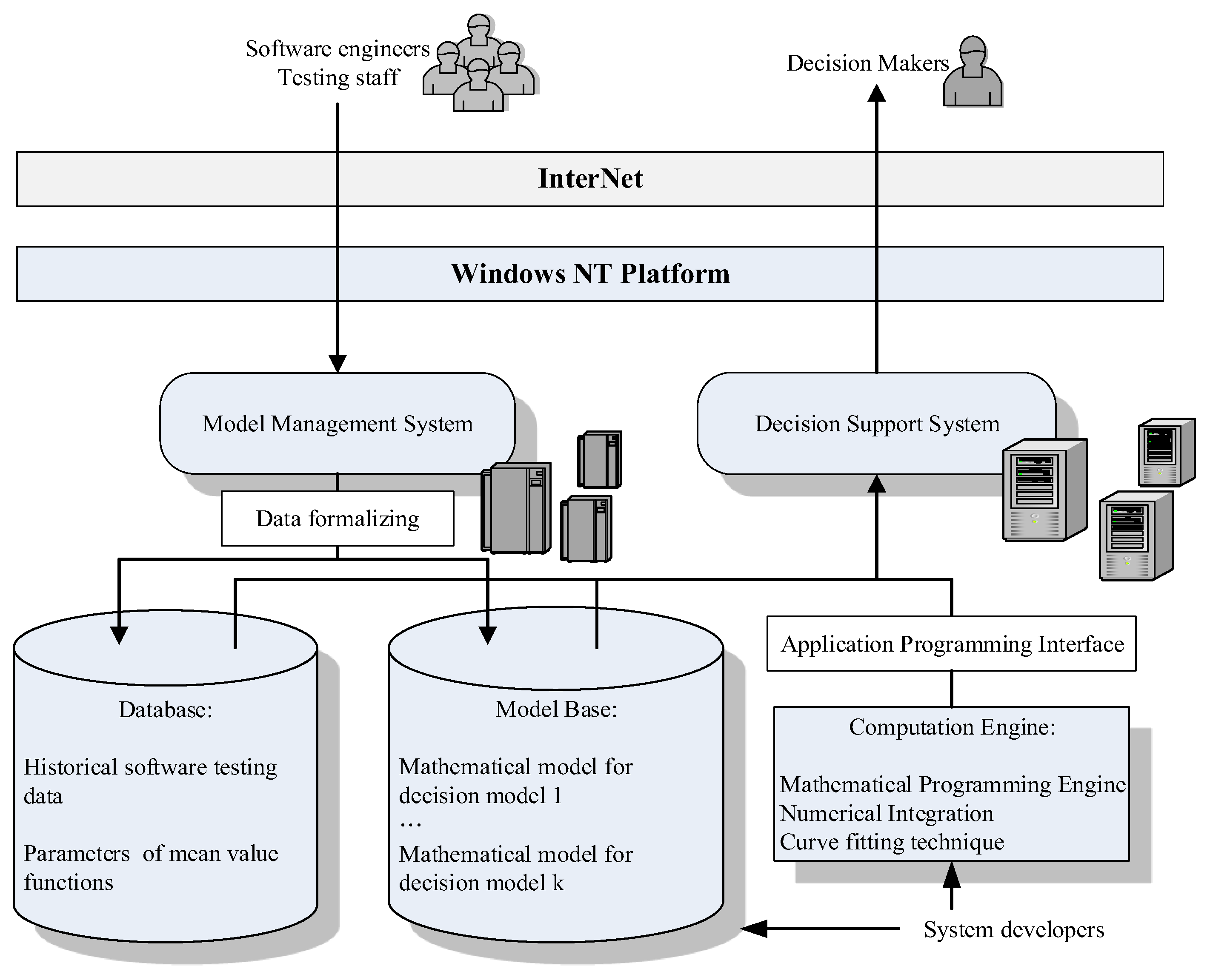
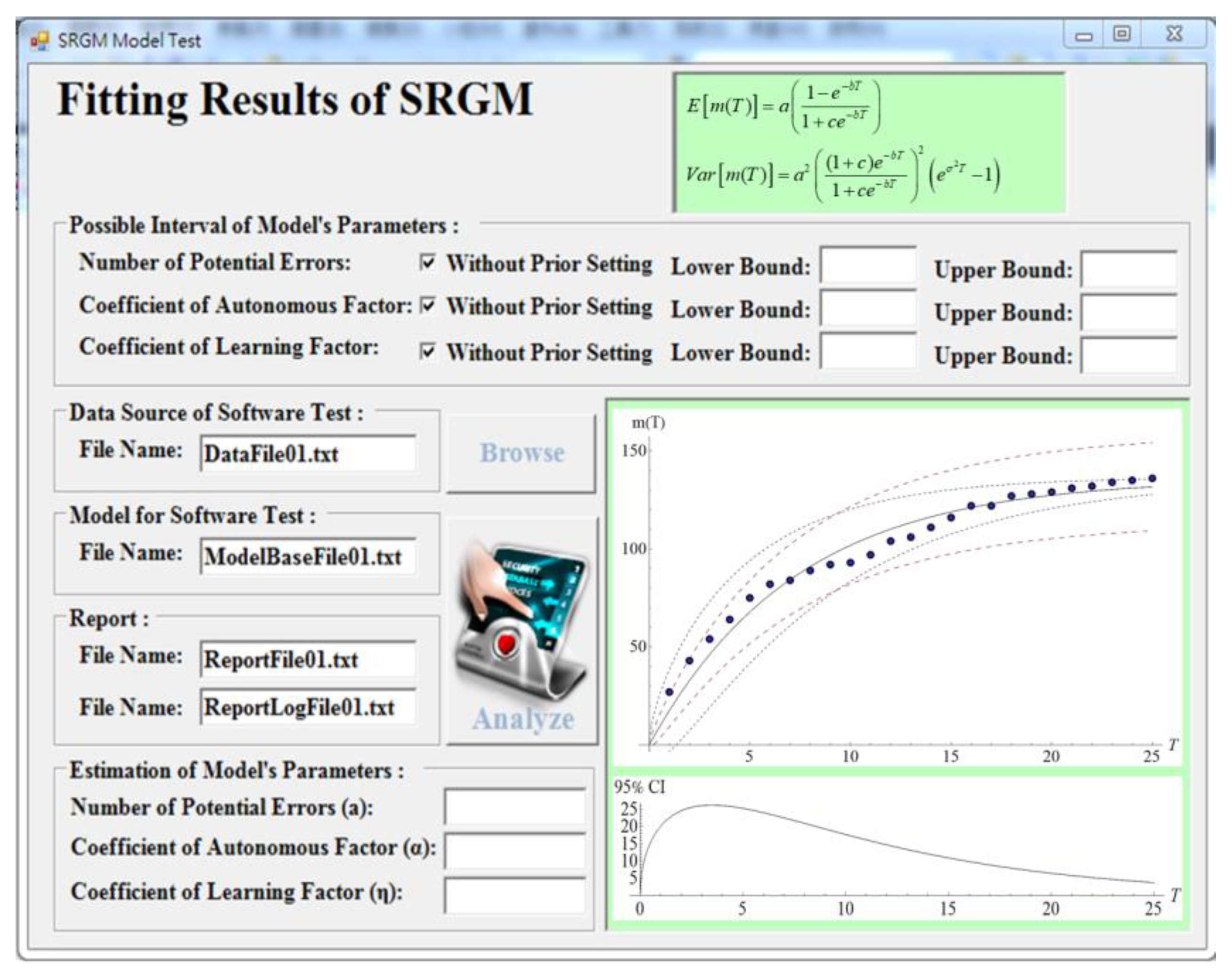
In this paper, Section 2 presents a brief literature review related to SRGMs. Section 3 explains Ohba’s SRGM that uses stochastic differential equations for the error detection rate. Estimation of the specification and validation of the result of the proposed model are also presented in this section. Section 4 describes an optimal software release model. Section 5 illustrates the architecture and the designed user interface of the decision support system for the proposed model. Section 6 summarizes the result of the model in this study to demonstrate its effectiveness. Lastly, the conclusions and suggestions for further research are presented in Section 7.

2. Literature Review

During testing and debugging, software reliability is useful for decision making. In the software industry, increasing reliability and reducing costs are the main goals [2]. The software developer needs to ensure the higher quality and the lower cost of the developed software as the most important objective during software development. Therefore, SRGMs are necessary to decide the release time of software and reduce its testing and debugging cost. Generally, SRGMs include exponential-shaped models, S-shaped models, or a mixture of both models [3].

NHP is commonly used to find the causes of the failure of software development. To illustrate the error detection of software development, Goel and Okumoto (1979) and Musa (1984) proposed exponential SRGMs in different aspects [4,5], which were generalizations or modifications of SRGMs. Musa, Yamada et al., and Yamada and Ohba respectively proposed exponential-shaped, S-shaped, and inflection S-shaped SRGMs for increasing the reliability of data testing [6,7,8]. For assessing the reliability, Pham and Zhang proposed an SRGM with combined estimations of testing and quality assurance [9]. Moreover, to analyze system reliability and performance, Huang tried to combine a logical testing effort function with change-point parameters to construct an SRGM [10].

The competitiveness of the project is determined by the timing of software release and quality and cost. Therefore, the accurate estimation of reliability and cost is subject to the efforts and resources of the testing project. SRGMs need to be reiterated on the basis of failure data. However, how programming designers learn from this during software testing and debugging is not considered in SRGMs. This learning effect affects the reliability of software without changing the cost of testing and debugging, as the experience of detecting errors according to the testers’ patterns is efficient. However, since software testing has uncertainties, the software developer needs to consider the risk and possible inaccuracy.

It is critical to understand a process of an accurate estimation of the confidence intervals of the mean value and the reliability of software. Most of the previous SRGMs adopted NHPP using the confidence interval of mean values. The confidence interval is calculated as $\widehat{m}\left(T\right)\pm Z_{CR/2}. \sqrt{\widehat{m}\left(T\right)}$, where CR is the critical region, $Z_{CR/2}$ is the critical value of a given area, and CR/2 is the standard normal distribution. Yamada and Osaki utilized different confidence intervals in their applications [11]. According to their study, the maximum likelihood method is efficient in estimating confidence intervals and related parameters. They considered a variance of testing time since the standard deviation is positively correlated with testing time. The confidence interval follows the assumption of NHPP; hence, they believed that the variance increased with the time for testing. However, as the occurrence of software defects is finite, the variance decreases as the testing time elapses. Therefore, the cumulative number of software errors decreases. This is different from the result of the estimation method of NHPP for hardware.

There have been efforts to improve the estimation of the confidence interval. Lee et al. and Tamura and Yamada thought that the variance is caused by the error detecting procedure, and the mean is estimated by stochastic differential equations (SDEs) [12,13]. Despite the effectiveness in assessing the mean value, the inference process still has problems. For instance, Ho et al. proposed an Itô-type SDE model with a changeable error detection rate [14]. Lee et al. (2004) extended the SRGMs [12] from Ohba [8] and Yamada [6] without the estimated variance. They used an Itô-type SDE method to improve the estimation of the confidence intervals so that a decision-maker can reasonably estimate the variability of software reliability and cost of testing software. Fang and Yeh [15] extended the SRGM of Tamura and Yamada [13] to propose flexible SDE models. However, their model did not obtain parameters; thus, the mean value and variance were not obtained.

Accurate estimation of risk is critical for software developers in deciding software release time. An SRGM assists decision-makers in finding the right timing for software release by estimating cost, system reliability, and required constraints. The environment for testing is important for software development and its release in time. Cortellessa et al. proposed an optimization-based approach to minimize costs on the basis of reliability and performance constraints [16]. Awad proposed to use software reliability and increased testing time to reduce system failure under limited time, resources, and cost [17]. According to Kooli et al. [18], there are differences in time and cost for reliability tests. Li and Pham suggested a reliability model based on the uncertainty in the operating environment [19]. The model determines the optimal release date of software with the reliability of software and testing cost. Zhu and Pham noted [20] that complete removal of software errors for each release is almost impossible due to limited resources. Thus, it is necessary to set an acceptable threshold for multiple software releases. Cao et al. proposed a model to minimize the cost of testing software and penalty after software releases [21]. A threshold was adopted for effectively determining the optimal time and cost of the software. Some imperfect systems regarding electronic circuits may also cause the risk of reliability [1]. Kim et al. [22] developed a software reliability model under the assumption that software failures occur in a dependent manner, which is different to the general assumption of independent manner. A policy of real-time software rejuvenation was proposed by Levitin et al. [23] by taking the distribution of transition times into account in the cost evaluation model.

On the basis of the previous study results, an improved model is proposed for the estimation of the mean and the confidence interval of system reliability and testing cost based on an SDE with an error detection function. It provides software developers with the relevant information for the risk management of software reliability and cost estimation.

3. Ohba’s DRGM with Stochastic Differential Equation

3.1. Model Development

SRGMs are effective in predicting the increase in software reliability. To fit the data into a model, the below SRGM based on NHPP is chosen. The methods of calculating error detection rate and mean value function are presented in

Table 1. Summary of previous models.

Model	Calculation of Error Detection Rate and Mean Value Function
Goel and Okumoto’s model	$D\left(t\right)=\beta$  $m\left(t\right)=a\left(1-e^{-\beta t}\right)$
Delayed, S-shaped model (Yamada)	$D\left(t\right)=\frac{{\beta }^{2}t}{1+\beta t}$  $m\left(t\right)=a\left(1-\left(1+\beta t\right)e^{-\beta t}\right)$
Musa’s exponential model	$D\left(t\right)=\frac{\gamma }{n\kappa }$  $m\left(t\right)=a\left(1-e^{-\left(\frac{\gamma t}{n\kappa }\right)}\right)$
Ohba’s inflection S-shaped model	$D\left(t\right)=\frac{\beta }{1+\gamma e^{-\beta t}}$  $m\left(t\right)=a\left(\frac{1-e^{-\beta t}}{1+\gamma e^{-\beta t}}\right)$

.

No method for calculating the confidence interval is presented in Table 1. Without it, software developers cannot estimate the increase in software reliability and cost in the testing and debugging process of software. Thus, we calculated confidence intervals using Ohba’s inflection S-shaped model as the confidence interval helps software developers evaluate potential changes in software reliability and cost to make a conservative decision for testing software. To obtain the confidence interval, the variance of the efficiency of debugging software is assumed to fluctuate with the detection rate of error and changes with testing time. The following notation is used to derive the proposed model in this study:

• $a$: the potential errors number are hidden in the system without any software debugging process;
• $m\left(t\right)$: the mean is calculated with the expected number of detected errors in the testing time range $\left(0,t\right)$;
• $\mathsf{\Phi }\left(t\right)$: the function of the residual error in a system at the testing time t and defined as $\mathsf{\Phi }\left(t\right)=a-m\left(t\right)$;
• $D\left(t\right)$: the error detection rate at testing time t;
• $\psi \left(t\right)$: the continuous-time stochastic process that indicates the magnitude of irregular fluctuations from the error detection rate $D\left(t\right)$;
• $\sigma$: the standard deviation of $\psi \left(t\right)$.

According to the definition of previous SRGMs, the error detection rate is regarded as the proportion of errors detected at time t and residual errors in a system. The rate is represented as $D\left(t\right)=\left(\frac{\mathrm{d}m\left(t\right)}{\mathrm{d}t}\right)/\left(a-m\left(t\right)\right)$. However, the fluctuation in the number of debugging software is not considered since the fluctuation originates from the function to calculate mean values. Therefore, we propose a new definition of fluctuation. In practice, the detection rate usually fluctuates during a test even with a trend due to the instability of human work. Accordingly, in debugging, the fluctuation of an error detection rate is presented as follows:

$$\frac{\frac{\mathrm{d}m(t)}{\mathrm{d}t}}{a-m(t)}=D(t)+\sigma \mathrm{d}\psi (t),$$

(1)

where $\psi \left(t\right)$ denotes the irregular fluctuations of the error detection rate. To deduce and solve the above equation smoothly, we define the function $\mathsf{\Phi }\left(t\right)$ that is equal to $a-m\left(t\right)$. Therefore, substituting $\mathsf{\Phi }\left(t\right)$ for $a-m\left(t\right)$ transforms Equation (1) to

$$\frac{\frac{\mathrm{d}\mathsf{\Phi }(t)}{\mathrm{d}t}}{\mathsf{\Phi }(t)}=-\left(D(t)+\sigma \mathrm{d}\psi (t)\right).$$

(2)

Taking a logarithm of $\mathsf{\Phi }\left(t\right)$ and making it equal to $\mathsf{\Omega }\left(t\right)$, the following equation is obtained with Itô’s method:

$$\frac{\frac{\mathrm{d}\mathsf{\Phi }(t)}{\mathrm{d}t}}{\mathsf{\Phi }(t)}=\mathrm{d}\mathsf{\Omega }(t)=\left\{-D(t)-\frac{1}{2}{\sigma }^2\right\}\mathrm{d}t-\sigma \mathrm{d}\psi (t)\left(\because \mathsf{\Omega }(t)=\ln \left[\mathsf{\Phi }(t)\right]\right).$$

(3)

As the integral of the derivative of $\mathsf{\Omega }\left(t\right)$ from 0 to $T$, $\mathsf{\Omega }\left(\mathrm{t}\right)$ is defined as

$${\displaystyle {\mathsf{\int }}_0^T\mathrm{d}\mathsf{\Omega }}(t)={\mathsf{\Omega }(t)|}_0^T=-{\displaystyle {\int }_0^{T}D(t)\mathrm{d}t}-{\displaystyle {\mathsf{\int }}_0^T\frac{1}{2}{\sigma }^2\mathrm{d}t}-{\displaystyle {\mathsf{\int }}_0^T\sigma \mathrm{d}\psi (t)},$$

(4)

where $\underset{0}{\overset{T}{{\displaystyle \mathsf{\int }}}}D\left(t\right)\mathrm{d}t$ is as follows:

$${\displaystyle {\int }_0^{T}D(t)\mathrm{d}t}=-\ln \left[\frac{(1+\gamma )e^{-\beta T}}{1+\gamma e^{-\beta T}}\right].$$

(5)

Therefore, Equation (4) is arranged as

$${\mathsf{\Omega }(t)|}_0^T=\ln \left[\frac{(1+\gamma )e^{-\beta T}}{1+\gamma e^{-\beta T}}\right]-{\displaystyle {\int }_0^T\frac{1}{2}{\sigma }^2\mathrm{d}t}-{\displaystyle {\int }_0^T\sigma \mathrm{d}\psi (t)}.$$

(6)

Since $\Omega \left(t\right)$ is equal to $\ln \left[\mathsf{\Phi }\left(t\right)\right]$, Equation (6) is rewritten as follows:

$$\ln \left[\mathsf{\Phi }(T)\right]=\ln \left[\frac{(1+\gamma )e^{-\beta T}}{1+\gamma e^{-\beta T}}\right]-{\displaystyle {\int }_0^T\frac{1}{2}{\sigma }^2\mathrm{d}t}-{\displaystyle {\int }_0^T\sigma \mathrm{d}\psi (t)}+c.$$

(7)

By solving Equation (7), $\mathsf{\Phi }\left(T\right)$ is defined as

$$\mathsf{\Phi }(T)=\frac{(1+\gamma )e^{-\beta T}}{1+\gamma e^{-\beta T}}{e}^{-\frac{1}{2}{\sigma }^{2}T-\sigma \psi (T)+c}.$$

(8)

$\mathsf{\Phi }\left(T\right)$ is for random variables that are normally distributed. To obtain the expected value of $\mathsf{\Phi }\left(T\right)$, Equation (8) needs to be further processed by applying the probability theory as follows:

$$E\left[\mathsf{\Phi }(T)\right]=E\left[\frac{(1+\gamma )e^{-\beta T}}{1+\gamma e^{-\beta T}}{e}^{-\frac{1}{2}{\sigma }^{2}T-\sigma \psi (T)+c}\right]=\frac{(1+\gamma )e^{-\beta T}}{1+\gamma e^{-\beta T}}{e}^{c-\frac{1}{2}{\sigma }^{2}T}E\left[e^{-\sigma \psi (T)}\right],$$

(9)

where $E\left[e^{-\sigma \psi \left(T\right)}\right]$ is deduced from ${{\displaystyle \int }}_{-\infty }^{\infty }\frac{1}{\sqrt{2\pi T}}{e}^{-\sigma x}{e}^{-\frac{x^2}{2T}}\mathrm{d}x=e^{\frac{1}{2}{\sigma }^{2}T}$. Then, Equation (8) is simplified as

$$E\left[\mathsf{\Phi }(T)\right]=\frac{(1+\gamma )e^{-\beta T}}{1+\gamma e^{-\beta T}}{e}^{c-\frac{1}{2}{\sigma }^{2}T}{e}^{\frac{1}{2}{\sigma }^{2}T}=\frac{(1+\gamma )e^{-\beta T}}{1+\gamma e^{-\beta T}}{e}^c.$$

(10)

Due to the initial condition of $\mathsf{\Phi }\left(0\right)=a$, the constant $c$ of the equations is equal to $\ln \left[a\right]$. Therefore, the expected mean, $E\left[m\left(T\right)\right]$ is obtained as follows:

$$E\left[m(T)\right]=E\left[a-\mathsf{\Phi }(T)\right]=a\left(\frac{1-e^{-\beta T}}{1+\gamma e^{-\beta T}}\right).$$

(11)

The variance of the mean $Var\left[m\left(T\right)\right]$ is defined as

$$Var\left[m(T)\right]=Var\left[\mathsf{\Phi }(T)\right]=E\left[\mathsf{\Phi }{(T)}^2\right]-E{\left[\mathsf{\Phi }(T)\right]}^2.$$

(12)

For obtaining $Var\left[m\left(T\right)\right]$, the value of $E\left[\mathsf{\Phi }{\left(T\right)}^2\right]$ needs to be calculated first. As given by Equation (7), $\mathsf{\Phi }\left(t\right)$ is used to obtain the real form of $E\left[\mathsf{\Phi }{\left(T\right)}^2\right]$. The following mathematical deduction leads to $E\left[\mathsf{\Phi }{\left(T\right)}^2\right]$:

$$\begin{array}{l}E\left[\mathsf{\Phi }{(T)}^2\right]=E\left[a^2{\left(\frac{(1+\gamma )e^{-\beta T}}{1+\gamma e^{-\beta T}}\right)}^2{e}^{-{\sigma }^{2}T-2\sigma \psi (T)}\right]\\ =a^2{\left(\frac{(1+\gamma )e^{-\beta T}}{1+\gamma e^{-\beta T}}\right)}^{2}E\left[e^{-{\sigma }^{2}T-2\sigma \psi (T)}\right]\end{array}.$$

(13)

Furthermore, as $E\left[e^{-2\sigma \psi \left(T\right)}\right]={{\displaystyle \int }}_{-\infty }^{\infty }\frac{1}{\sqrt{2\pi T}}{e}^{-2\sigma x}{e}^{-\frac{x^2}{2T}}\mathrm{d}x=e^{2{\sigma }^{2}T}$, Equation (13) is rewritten as

$$E\left[\mathsf{\Phi }{(T)}^2\right]=a^2{\left(\frac{(1+\gamma )e^{-\beta T}}{1+\gamma e^{-\beta T}}\right)}^2{e}^{{\sigma }^{2}T}.$$

(14)

Similarly, since $E\left[\mathsf{\Phi }\left(T\right)\right]=a\left(e^{-{{\displaystyle \int }}_0^{T}D\left(t\right)\mathrm{d}t}\right)$, $E{\left[\mathsf{\Phi }\left(T\right)\right]}^2$ is defined as

$$E{\left[\mathsf{\Phi }(T)\right]}^2={\left(a\left(\frac{(1+\gamma )e^{-\beta T}}{1+\gamma e^{-\beta T}}\right)\right)}^2.$$

(15)

On the basis of Equations (14) and (15), the variance $Var\left[\mathsf{\Phi }\left(T\right)\right]$ of the mean value is obtained as

$$\begin{array}{ll}Var\left[\mathsf{\Phi }(T)\right]& =E\left[\mathsf{\Phi }{(T)}^2\right]-E{\left[\mathsf{\Phi }(T)\right]}^2\\ & =a^2\left(e^{{\sigma }^{2}T}-1\right){\left(\frac{(1+\gamma )e^{-\beta T}}{1+\gamma e^{-\beta T}}\right)}^2=\left(e^{{\sigma }^{2}T}-1\right){\left(a-m(T)\right)}^2\end{array}.$$

(16)

Since $Var\left[m\left(T\right)\right]$ is mapping $Var\left[\mathsf{\Phi }\left(T\right)\right]$, $Var\left[m\left(T\right)\right]=Var\left[\mathsf{\Phi }\left(T\right)\right]$ according to Equation (11).

Even with the expected and the variance of the mean, practical application is required for software developers. Section 3.3 describes how confidence intervals are applied to the decision making of the release time of software considering the testing cost and required reliability. Since the parameter of Ohba’s inflection S-shaped model needs to be estimated, Section 3.2 presents the least-squares estimation (LSE) and the maximum likelihood estimation (MLE) for the proposed model.

3.2. Estimating Parameters

LSE and MLE are proposed for estimating the parameters $\beta$, $\gamma$, and $a$ [24]. The MLE is used to estimate the parameters of a probability distribution by a maximized likelihood function. Suppose that the set of paired data $\left(T_i,m_i\right)$ is collected where $m_i$ is the detected number of errors until $T_i$. It is assumed that the unknown parameters of the specified SRGMs are obtained by the observed pairwise data $\left(m_0,T_0\right),\left(m_1,T_1\right),\left(m_2,T_2\right),\left(m_3,T_3\right),\dots ,\left(m_n,T_n\right)$. Therefore, the likelihood function of SRGMs is expressed as follows:

$$\begin{array}{ll}f(\beta ,\gamma ,a|T_i)& =\mathrm{Pr}\{\mathsf{\Delta }(T_1)=m_1,\mathsf{\Delta }(T_2)=m_2,\mathsf{\Delta }(T_3)=m_3,\dots ,\mathsf{\Delta }(T_n)=m_n\}\\ & ={\displaystyle \prod _{i=1}^n\left(e^{-(m(T_i)-m(T_{i-1}))}\right)\frac{{\left(m(T_i)-m(T_{i-1})\right)}^{(m_i-m_{i-1})}}{(m_i-m_{i-1})!}}\end{array}$$

(17)

To find the MLE, the likelihood function in Equation (17) is taken on the logarithmic scale as follows:

$$\begin{array}{ll}\ln \left[f(\beta ,\gamma ,a|T_i)\right]& ={\displaystyle \sum _{i=1}^n(m_i-m_{i-1})\ln \left[m(T_i)-m(T_{i-1})\right]}\\ & -{\displaystyle \sum _{i=1}^n\ln \left[(m_i-m_{i-1})!\right]}-{\displaystyle \sum _{i=1}^n\left(m(T_i)-m(T_{i-1})\right)}\end{array}.$$

(18)

On the basis of the above equation, the MLE of the model’s parameters $\widehat{\beta }$, $\widehat{\gamma }$, and $\widehat{a}$ is attained through the equation $\frac{\partial \ln [f(\beta ,\gamma ,a|T_i)]}{\partial \beta }=\frac{\partial \ln [f(\beta ,\gamma ,a|T_i)]}{\partial \gamma }=\frac{\partial \ln [f(\beta ,\gamma ,a|T_i)]}{\partial a}=0$.

Furthermore, LSE is also used to estimate the model’s parameters. The evaluation function of the LSE is presented as

$$\mathrm{Min}\begin{array}{c}\end{array}{\displaystyle \sum _{i=1}^n{\left(m_i-m(T_i)\right)}^2}.$$

(19)

Similarly, the LSE for the parameters $\widehat{\beta }$, $\widehat{\gamma }$, and $\widehat{a}$ is obtained by solving the simultaneous equations $\frac{\partial \left[{{\displaystyle \sum }}_{i=1}^n{\left(m_i-m\left(T_i\right)\right)}^2\right]}{\partial \beta }=\frac{\partial \left[{{\displaystyle \sum }}_{i=1}^n{\left(m_i-m\left(T_i\right)\right)}^2\right]}{\partial \gamma }=\frac{\partial \left[{{\displaystyle \sum }}_{i=1}^n{\left(m_i-m\left(T_i\right)\right)}^2\right]}{\partial a}=0$.

Moreover, the standard deviation of $\psi \left(t\right)$ is significant for measuring the confidence interval. Therefore, ${\widehat{\sigma }}^2$ needs to be determined. The relationship between $\sigma$ and $Var\left[m\left(T\right)\right]$ is recognized in Equation (16), thus defining the following equation:

$${\widehat{\sigma }}^2=\frac{1}{\left(n-k\right)}{\displaystyle \sum _{i=1}^n\left(1/T_i\right)\ln \left[\frac{{\left(m_i-m\left(T_i\right)\right)}^2}{{\left(\widehat{a}-m\left(T_i\right)\right)}^2}+1\right]},$$

(20)

where $k$ represents the number of the estimated parameters. On the basis of the above equations, the confidence interval of the mean and the corresponding software reliability are explained in the next section.

3.3. Estimating Confidence Intervals of Mean and Software Reliability

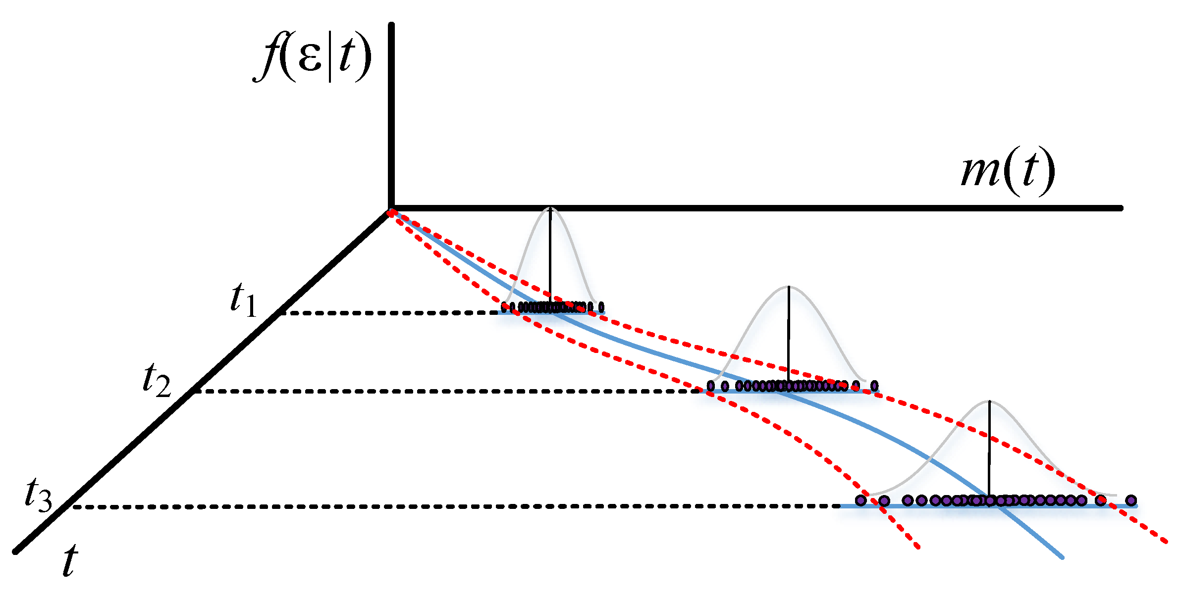
For the estimation of confidence intervals of SRGMs, many previous studies adopted Yamada and Osaki’s estimation method [11]. The estimation was developed for hardware reliability with the assumption of gradual increase and instability of the failure rate. The traditional method of estimating the confidence interval is as follows:

$$\mathrm{Upper} \mathrm{Bound} m_{UB}^{CR}(T): m(T)+\sqrt{m(T)}{\mathrm{Z}}_{CR/2},$$

(21)

$$\mathrm{Lower} \mathrm{Bound} m_{LB}^{CR}(T): m(T)-\sqrt{m(T)}{\mathrm{Z}}_{CR/2}.$$

(22)

$CR$ and $\sqrt{m\left(T\right)}$ denote the critical region and standard deviation, respectively. ${\mathrm{Z}}_{CR/2}$ represents the value of critical region $CR/2$ that follows a standard normal distribution. As the standard deviation (SD) $\sqrt{m\left(T\right)}$ is correlated with time $T$ positively, the confidence interval is enlarged during the test. However, in reality, the failure rate during the software debugging gradually decreases and becomes stable as the failures are removed during a testing period. Accordingly, it is inappropriate to apply Yamada and Osaki’s method.

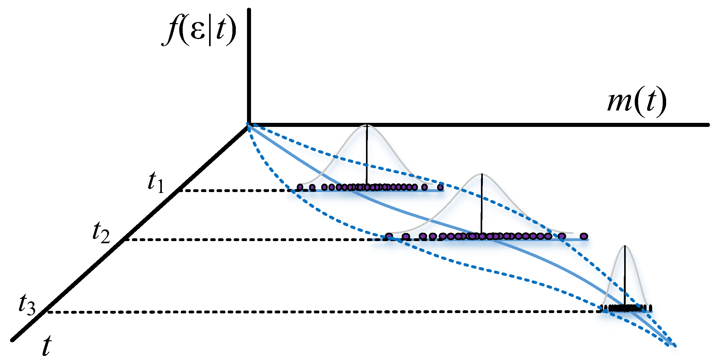
Therefore, the confidence interval is proposed with a consideration that the variance of efficiency of debugging depends on the error detection rate. By applying the abovementioned equations, the upper and lower boundaries of the confidence interval for the mean are calculated as follows:

$$\begin{gathered} \mathrm{Upper} \mathrm{Bound} m_{UB}^{CR}(T): \\ E\left[m(T)\right]+{\left(Var[m(T)]\right)}^{1/2}{\left(1+1/n+{\left(T-\overline{t}\right)}^2/{\displaystyle \sum _{i=1}^n{\left(t_i-\overline{t}\right)}^2}\right)}^{1/2}{t}_{CR/2,n-k}, \end{gathered}$$

(23)

$$\begin{gathered} \mathrm{Lower} \mathrm{Bound} m_{LB}^{CR}(T): \\ E\left[m(T)\right]-{\left(Var[m(T)]\right)}^{1/2}{\left(1+1/n+{\left(T-\overline{t}\right)}^2/{\displaystyle \sum _{i=1}^n{\left(t_i-\overline{t}\right)}^2}\right)}^{1/2}{t}_{CR/2,n-k}, \end{gathered}$$

(24)

where $t_{CR/2,n-k}$ represents the critical region $CR/2$ of Student’s t probability distribution with $n-k$ degrees of freedom. For simplifying the equations, the upper and lower boundaries of the mean are denoted as $m_{UB}^{CR}\left(T\right)$ and $m_{LB}^{CR}\left(T\right)$.

Traditional methods consider that the variance of the errors comes from $m\left(T\right)$, while the proposed method assumes that the variance comes from $D\left(T\right)$. Thus, the confidence interval of the traditional model becomes divergent in the later stage of the testing work. However, the possibility of finding new software errors decreases with testing time since the software errors are found to be much less at the end of testing than at previous stages. In other words, the variance and the fluctuation of errors decrease with testing time when the remaining errors become fewer at the end-stage. Therefore, the variance and the fluctuation of errors vary with the error detection rate, converging at the end-stage. 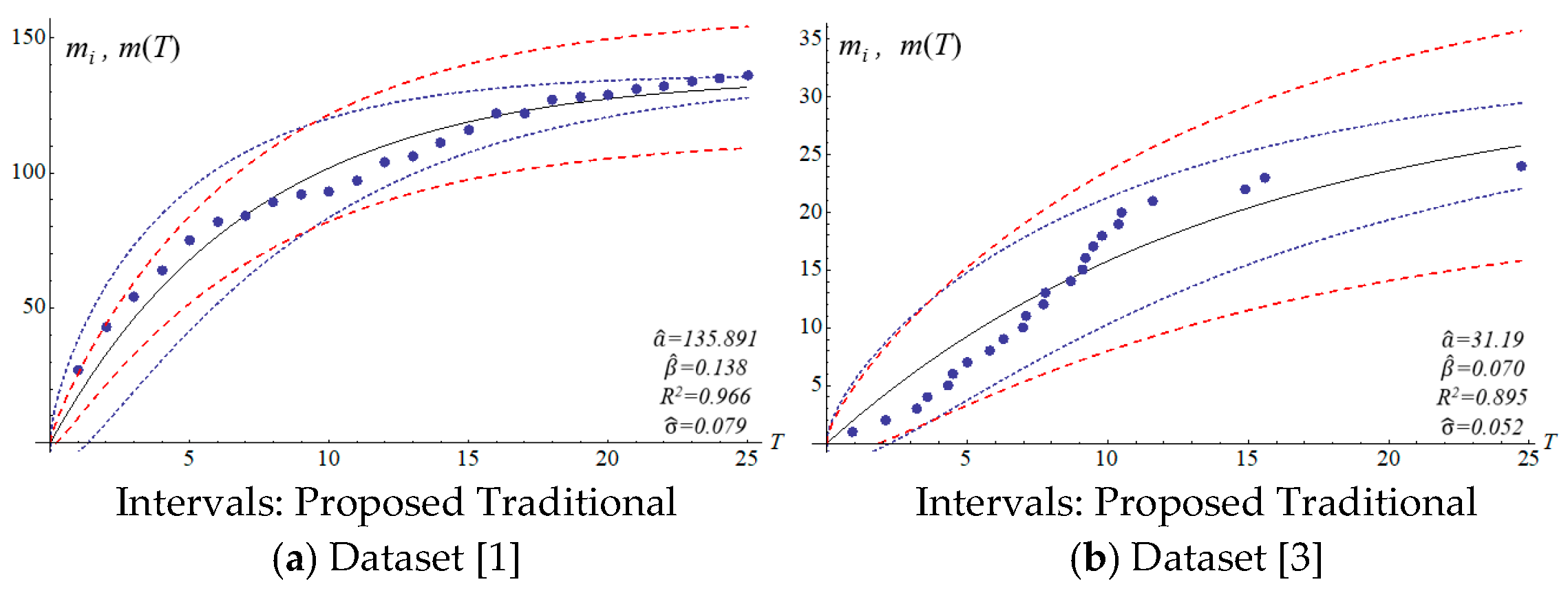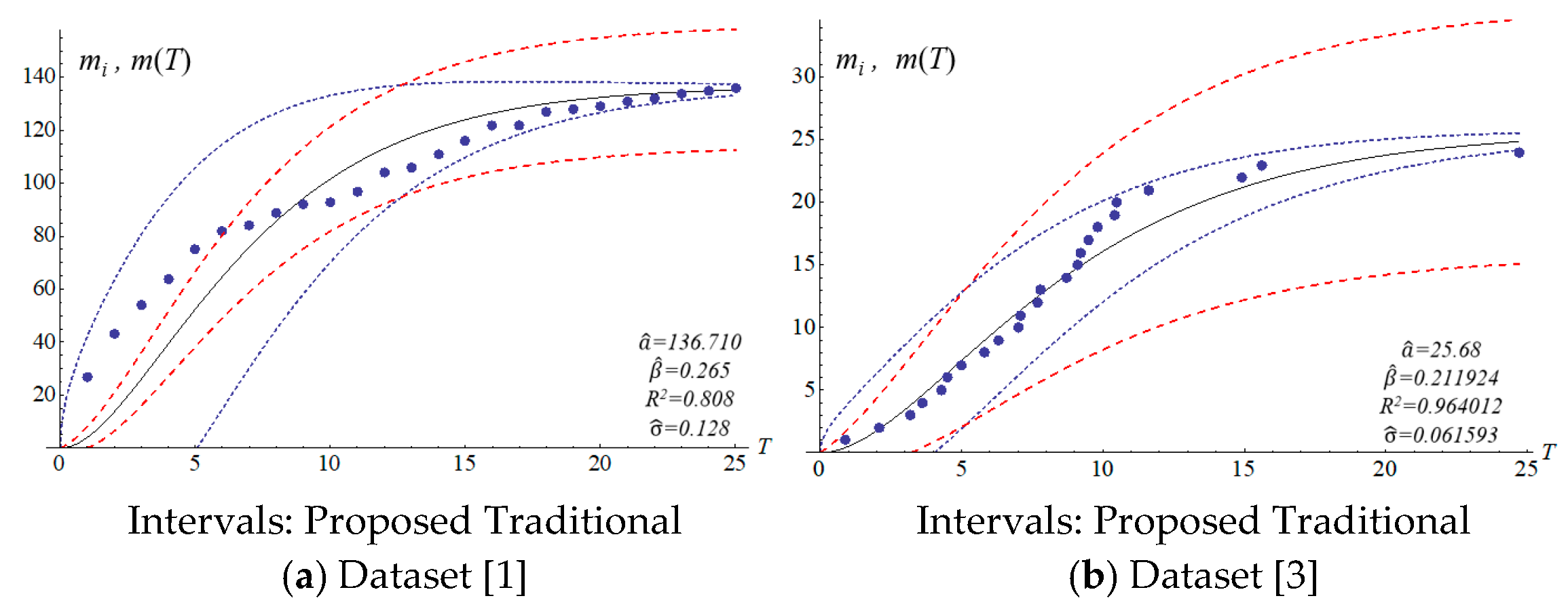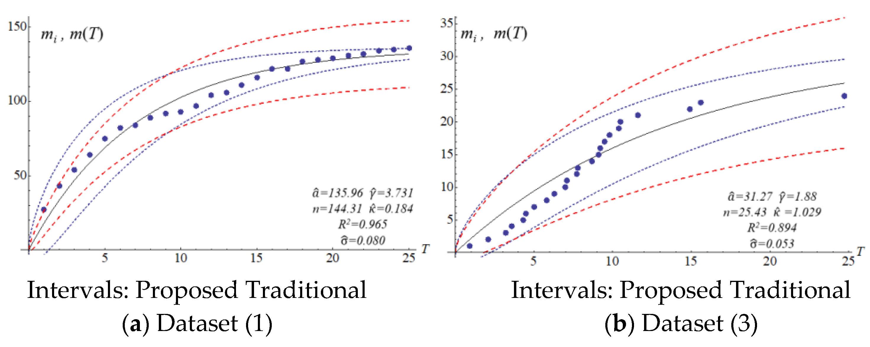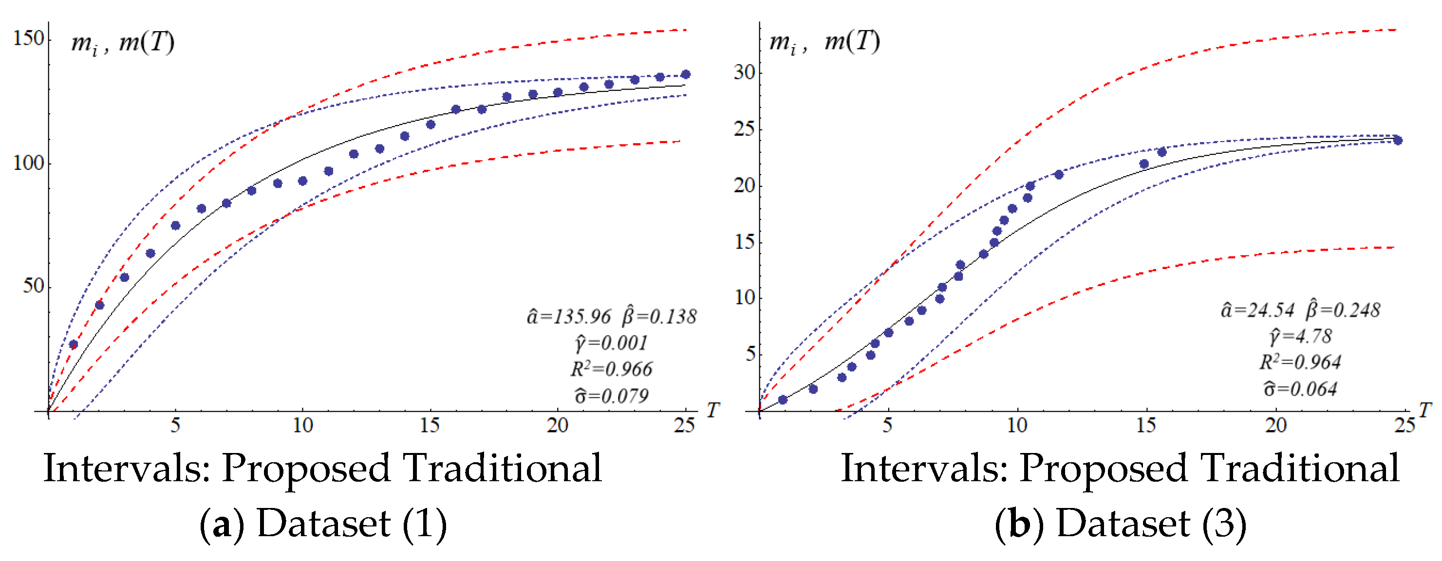Figure 1 and Figure 2 show the different confidence intervals between the traditional and proposed methods.

The reliability of software $R\left(x/T\right)$ is to measure the quality of a system software during a testing period, and the general definition is

$$R(x/T)=e^{-\left[m(T+x)-m(T)\right]}.$$

(25)

$R\left(x/T\right)$ is for the probability that no software error occurs during $\left[T, T+x\right]$, where $x$ is the predefined time of software operation. On the basis of Equation (25), the upper and lower boundaries of the reliability of software are inferred as follows:

$$\mathrm{Upper} \mathrm{Bound} R_{UB}^{CR}(x/T): e^{-\left[m_{UB}^{CR}(T+x)-m_{UB}^{CR}(T)\right]},$$

(26)

$$\mathrm{Lower} \mathrm{Bound} R_{LB}^{CR}(x/T): e^{-\left[m_{LB}^{CR}(T+x)-m_{LB}^{CR}(T)\right]}.$$

(27)

3.4. Model Validation

Various model parameters were validated in this section. Six datasets from different methods were used for evaluating the effectiveness of the estimation method in this study (

Table 2. Datasets for validation.

Dataset	Literature	Testing Dataset	Reference
(1)	Zhang and Pham (1998)	Failure dataset from Misra system	[25]
(2)	Shyur (2003)	Failure dataset from Misra system	[26]
(3)	Hossain and Dahiya (1993)	Failure dataset from NTDS system	[27]
(4)	Pham and Zhang (2003)	Failure dataset from Tandem software	[9]
(5)	Jeske and Zhang (2005)	Failure dataset from wireless data service system	[28]
(6)	Zhang and Pham (2006)	Failure dataset from telecommunication system	[29]

).

We applied the six datasets to four SRGMs to estimate their confidence intervals.

Table 3. Estimated values of parameters for classic models and software testing datasets.

Testing Dataset	Goel and Okumoto Model	Yamada’s Delayed S-Shaped Model	Musa’s Exponential Model	Ohba Inflection S-Shaped Model (Proposed Model)
(1)	$\widehat{a }$= 135.891 $\widehat{\beta }$= 0.138 R2 = 0.966 $\widehat{\sigma }$= 0.079	$\widehat{a}$= 136.710 $\widehat{\beta }$= 0.265 R2 = 0.808 $\widehat{\sigma }$= 0.128	$\widehat{a}$= 135.96  $\widehat{\gamma }$= 3.731 n = 144.31  $\widehat{\kappa }$= 0.184 R2 = 0.965 $\widehat{\sigma }$= 0.080	$\widehat{a}$= 135.96  $\widehat{\beta }$= 0.138 $\widehat{\gamma }$= 0.001 R2 = 0.966 $\widehat{\sigma }$= 0.079
(2)	$\widehat{a}$= 164.47 $\widehat{\beta }$= 0.063 R2 = 0.976 $\widehat{\sigma }$= 0.0273	$\widehat{a}$= 148.19 $\widehat{\beta }$= 0.174546 R2 = 0.948113 $\widehat{\sigma }$= 0.0601241	$\widehat{a}$= 165.61  $\widehat{\gamma }$= 1.677 n = 156.49  $\widehat{\kappa }$= 0.166 R2 = 0.975 $\widehat{\sigma }$= 0.0267	$\widehat{a}$= 184.88  $\widehat{\beta }$= 0.071 $\widehat{\gamma }$= 0.556 R2 = 0.990 $\widehat{\sigma }$= 0.016
(3)	$\widehat{a}$= 31.19 $\widehat{\beta }$= 0.070 R2 = 0.895 $\widehat{\sigma }$= 0.052	$\widehat{a }$= 25.68 $\widehat{\beta }$= 0.211924 R2 = 0.964012 $\widehat{\sigma }$= 0.061593	$\widehat{a }$= 31.27  $\widehat{\gamma }$= 1.88 n = 25.43  $\widehat{\kappa }$= 1.029 R2 = 0.894 $\widehat{\sigma }$= 0.053	$\widehat{a}$= 24.54  $\widehat{\beta }$= 0.248 $\widehat{\gamma }$= 4.78 R2 = 0.964 $\widehat{\sigma }$= 0.064
(4)	$\widehat{a}$= 122.64 $\widehat{\beta }$= 0.017 R2 = 0.987 $\widehat{\sigma }$= 0.011	$\widehat{a}$= 101.90 $\widehat{\beta }$= 0.050708 R2= 0.947729 $\widehat{\sigma }$= 0.040946	$\widehat{a }$= 122.77  $\widehat{\gamma }$= 1.850 n = 106  $\widehat{\kappa }$= 1 R2 = 0.988 $\widehat{\sigma }$= 0.011	$\widehat{a}$= 121.61  $\widehat{\beta }$= 0.020 $\widehat{\gamma }$= 0.275 R2 = 0.990 $\widehat{\sigma }$= 0.011
(5)	$\widehat{a}$= 22.86 $\widehat{\beta }$= 0.542 R 2= 0.984 $\widehat{\sigma }$= 0.108	$\widehat{a }$= 21.76 $\widehat{\beta }$= 1.361881 R2 = 0.964143 $\widehat{\sigma }$= 0.343911	$\widehat{a}$= 22.72  $\widehat{\gamma }$= 3.76511 n= 23.41  $\widehat{\kappa }$= 0.291 R2 = 0.986 $\widehat{\sigma }$= 0.106	$\widehat{a}$= 21.88  $\widehat{\beta }$= 0.788 $\widehat{\gamma }$= 0.486 R2 = 0.987 $\widehat{\sigma }$= 0.210
(6)	$\widehat{a }$= 134.41 $\widehat{\beta }$= 0.098 R2 = 0.864 $\widehat{\sigma }$= 0.078	$\widehat{a }$= 134.82 $\widehat{\beta }$= 0.246786 R2 = 0.974 $\widehat{\sigma }$= 0.033	$\widehat{a }$= 133.19  $\widehat{\gamma }$= 1.062 N = 105  $\widehat{\kappa }$= 0.1 R2 = 0.865 $\widehat{\sigma }$= 0.081	$\widehat{a}$= 111.68  $\widehat{\beta }$= 0.468 $\widehat{\gamma }$= 13.498 R2 = 0.990 $\widehat{\sigma }$= 0.038

presents the estimated parameters.

The four SRGMs and two datasets were used to compare the confidence interval of the models to that of the proposed model. Datasets (1) and (3) in Table 2 present the data distribution of a concave and an S-shape, respectively. Figure 3, Figure 4, Figure 5 and Figure 6 show that the variation of the confidence interval changes. The blue and red dashed lines of the figures respectively represent the estimation of confidence intervals for the traditional and proposed models. Results from the comparison show large differences in confidence intervals. The models of Goel and Okumoto and Musa with datasets (3) and (6) show R-squared values (0.8–0.9) that are not satisfactory. There are discrepancies in the distribution of dataset (3) in Figure 3b and Figure 5b. Thus, the model’s accuracy needs to be determined by the scatter pattern in the dataset. Accordingly, the performance of model fitting may depend on the pattern of a dataset. A model may fit for some datasets but it may not fit for all the datasets. In other words, both Goel and Okumoto’s and Musa’s models have a constant detection rate which is opposite to the scenario of a nonconstant detection rate of the Yamada model and the proposed model (Figure 3 and Figure 6). As a result, the detection rates for Goel and Okumoto’s and Musa’s models cannot be used to predict the pattern of S-shaped datasets. However, Yamada’s delayed S-shaped model and Ohba’s inflection model (the proposed model) are able to accurately estimate all the datasets with S-shaped or concave datasets. In summary, the proposed confidence interval converges with the testing time to reflect the actual situation. The number of software errors decreases with testing/debugging time. Figure 3, Figure 4, Figure 5 and Figure 6 present that the difference between actual and estimated errors is the greatest when the testing/debugging process begins and then decreases with time. After debugging and testing, the actual number and the estimated number of software errors are almost identical. When compared with the traditional models, the estimation of the proposed model shows a narrower 95% confidence interval. For example, the confidence intervals for the traditional models are large and are not indicative of datasets (1) or (3).

4. Decision with Confidence Levels

Software developers aim to reduce the cost of development and secure the quality of software by deciding when testing is completed and software is released. In general, a longer testing period results in more reliable software. However, a software developer cannot prolong the testing period indefinitely as this increases the costs and loses business opportunities. Therefore, a software developer considers a trade-off between testing period and software quality. Zhang and Pham suggested a cost–reliability model for the best policy for software releases [25]. Thus, the model was adopted in this study to develop a software release model based on different confidence levels. The proposed cost–reliability model has the following six factors in deciding when to release the software:

(1)

Setup cost ($StC$) for testing concerning necessary equipment and initial investment before the testing project begins;

(2)

Routine expense ($RtC\left({\theta }_{Rt},T\right)$) for testing including salary, insurance, rent, and so on during a planned testing period $\left[0,T\right]$. ${\theta }_R$ denotes the routine expense per unit time, and the routine expense is calculated by ${\theta }_{Rt}T$;

(3)

Debugging expense ($DC\left({\theta }_E,{\xi }_E,m\left(T\right)\right)$) for removing software errors during a planned testing period $\left[0,T\right]$. The estimation of the expense is related to the expense of omitting an error per unit time ${\theta }_E$ and the average required time to delete an error ${\xi }_E$. Therefore, the debugging expense is calculated by ${\rho }_{E}m\left(T\right){\xi }_E$;

(4)

The cost of risk of a software failure after its release ($RkC\left({\theta }_{Rk},R\left(x/T\right)\right)$ is estimated by ${\theta }_{Rk}\left(1-R\left(x/T\right)\right)$. The parameter ${\theta }_{Rk}$ is calculated by estimating how much risk cost for users or customers is caused by the 1% loss of software reliability at release time $T$;

(5)

Opportunity cost ($OpC\left({\theta }_O,{\varpi }_1,{\varpi }_2,T\right)$), as tangible and intangible losses caused by postponing software release, is defined as ${\theta }_O{\left({\varpi }_1+T\right)}^{{\varpi }_2}$ in this study. ${\varpi }_1$ and ${\varpi }_2$ are parameters for the power-law function, estimated by marketing experts. ${\theta }_O$ denotes the scale for base opportunity cost;

(6)

Minimal requirement of software reliability $R_0$ is a standard indicator for the requirement of users or customers for which the operation of a software system must meet.

By considering the factors, the software release model for the average case is presented as follows:

$$\begin{array}{ll}Minimize TC\left(T\right)=StC& +RtC\left({\theta }_{Rt},T\right)+DC\left({\theta }_E,{\xi }_E,m(T)\right)\\ & +RkC\left({\theta }_{Rk},R(x/T)\right)+OpC\left({\theta }_O,{\varpi }_1,{\varpi }_2,T\right)\\ Subject to: R(x/T)\ge R_0\end{array}$$

(28)

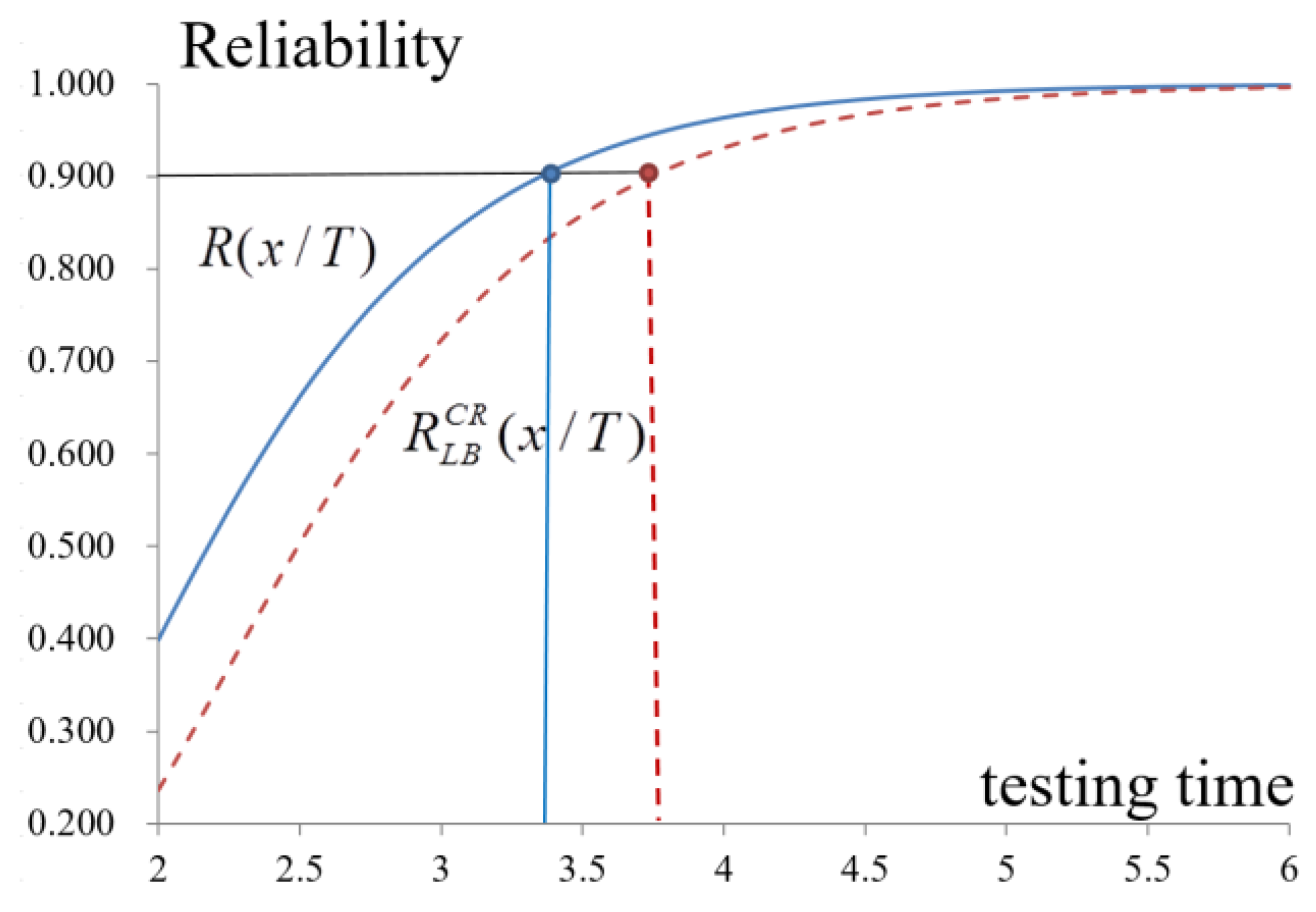
Since the model is only for a general case, decision-makers cannot effectively evaluate the potential risk due to the extension of the testing schedule. Various possibilities of the delay need to be considered to handle the extra cost and prepare for postponing the software release. The reliability of software does not reach the desired level in most testing cases. Thus, decision-makers need conservative estimations for the cost and reliability, which leads to the consideration of the worst case in making decisions. Thus, according to Equation (28), the lower bound estimation $m_{LB}^{CR}\left(T\right)$ and $R_{LB}^{CR}\left(x/T\right)$ at a specific confidence level, $CR$ was taken into consideration to apply the decision model in this study. Equation (29) presents the proposed decision model. Decision-makers can use this model by setting an appropriate confidence level to determine the best release time of the software.

$$\begin{array}{ll}Minimize T{C}_{LB}^{CR}\left(T\right)=& StC+RtC\left({\theta }_{Rt},T\right)+DC\left({\theta }_E,{\xi }_E,m_{LB}^{CR}(T)\right)\\ & +RkC\left({\theta }_{Rk},R_{LB}^{CR}(x/T)\right)+OpC\left({\theta }_O,{\varpi }_1,{\varpi }_2,T\right)\\ Subject to: R_{LB}^{CR}(x/T)\ge R_0\end{array}$$

(29)

5. Computerized Implementation Architecture

5.1. Model Development

To effectively apply the result of this study, a computerized system is necessary for a problem-solving process. In this study, components such as an organized database, a model base, data formalizing modules, a specific application programming interface, and a designed computation engine are included in the system.

The database is designed to store the related costs, failure data of various systems, and experts’ inputs. A model base is created for the software growth model and the mathematical model to assess the impacts of different software release policies. By storing and/or accessing the database and model base, the formalized data structure is used to find the inconsistent data. The system has more efficiency and effectiveness in storing and accessing the formalized data than previous ones.

The proposed model requires programming algorithms and numerical integration methods. A powerful computation capability is needed to construct the system. The computation engine is developed by programmers or obtained from external software providers (e.g., from Python packages or Lingo Systems). To utilize a computation engine efficiently and conveniently, an appropriate mechanism of a programming interface is necessary for exchanging information among the components of the designed system.

5.2. System Design and Operation

The entire system is composed of two subsystems. Domain experts, software engineers, and testing staff need to provide various models and parameters for the model management system for enhancing applicability and manageability. The decision support system provides the relevant information for testing staff to make effective decisions. The operating system requires the engineers or testing staff to collect all relevant data in advance. They need to investigate all critical parameters, cost structures, previous testing data, and mathematical models to input into the system. The efficiency of software testing is important in determining the software release timing and estimating the testing cost. Therefore, domain experts need to choose and evaluate which SRGM is suitable for the current project. Moreover, all the engineers, domain experts, and managers are allowed to access their subsystems only because of commercial confidentiality. For upper-level management, the decision support system offers complete and integrated information to assist them in making the best decision. Decision-makers examine all constructive information in the database and model base to determine the optimal decision. To obtain an optimal decision, computation is required; hence, computation programs need to be developed. The system’s structure is shown in Figure 7, and an example of the system’s interface is presented in Figure 8.

6. Discussions

A software service provider develops commercial software applications. When the coding is completed, the service provider’s manager determines an appropriate release date. The inflection S-shape model by Ohba is appropriate for the determination based on historical data and expert evaluation. According to the potential error, the model has a standard deviation of $\widehat{\sigma }$ = 0.228, a potential error of $\widehat{a}$ up to 3350, parameter $\widehat{\gamma }$ of 0.015, and parameter $\widehat{\beta }$ of 1.35. In detecting errors, each employee works 10 h a day and 24 days a month, which pertains to $StC$= $2000, ${\theta }_{Rt}$= $6000, ${\theta }_E$= $12,000, ${\theta }_{Rk}$= $252,000, ${\theta }_O$= $3800, $x$= 1 h, ${\varpi }_1$= 2, ${\varpi }_2$= 1.6, and ${\xi }_E$= 0.5 h. As a software service provider wants to meet a minimum software reliability requirement ($R_0$= 0.9) at the confidence level of 95%, they need to identify the optimal software release time for general and worst cases.

By using spectrum analysis with Equations (28) and (29), when to release a software package, the expected cost of testing, and the safety of the software package before release are determined.

Table 4. Values of $R\left(x/T\right), TC\left(T\right), R_{LB}^{CR}\left(x/T\right)$ and $T{C}_{LB}^{CR}\left(T\right)$ vs. testing time.

Average Case			Worst Case (Confidence Level = 0.95)
T (months)	$\mathit{R}\left(\mathit{x}/\mathit{T}\right)$	$\mathit{E}\left[\mathit{C}\left(\mathit{T}\right)\right]$	T (Months)	${\mathit{R}}_{\mathit{L}\mathit{B}}^{\mathit{C}\mathit{R}}\left(\mathit{x}/\mathit{T}\right)$	${\mathit{E}}_{\mathit{L}\mathit{B}}^{\mathit{C}\mathit{R}}\left[\mathit{C}\left(\mathit{T}\right)\right]$
3	0.830	281,040	3	0.723	306,685
3.05	0.842	279,303	3.05	0.740	303,711
3.1	0.854	277,754	3.1	0.757	300,946
3.15	0.864	276,385	3.15	0.772	298,387
3.2	0.874	275,186	3.2	0.787	296,029
3.25	0.883	274,149	3.25	0.801	293,867
3.3	0.891	273,264	3.3	0.814	291,896
3.35	0.899	272,524	3.35	0.826	290,109
3.4	0.907	271,921	3.4	0.838	288,499
3.45	0.913	271,446	3.45	0.849	287,060
3.5	0.920	271,091	3.5	0.859	285,783
3.55	0.926	270,850	3.55	0.868	284,663
3.6	0.931	270,716	3.6	0.877	283,691
3.65	0.936	270,682 *	3.65	0.886	282,860
3.7	0.941	270,741	3.7	0.894	282,164
3.75	0.946	270,888	3.75	0.901	281,595
3.8	0.950	271,117	3.8	0.908	281,147
3.85	0.953	271,422	3.85	0.914	280,813
3.9	0.957	271,800	3.9	0.920	280,587
3.95	0.960	272,244	3.95	0.926	280,462
4	0.963	272,752	4	0.931	280,434 *
4.05	0.966	273,318	4.05	0.936	280,496
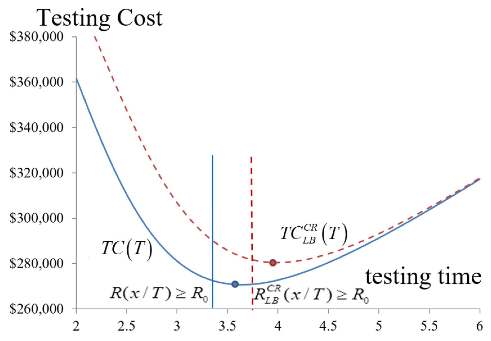
4.1	0.971	273,938	4.1	0.941	280,642

and Figure 9 show that the optimized release time for software, ${{\rm T}}^{\ast }$, is 3.65 months after the beginning of debugging and testing. The total cost and the reliability are estimated to be approximately $270,682 and 0.936 in the general case to satisfy the requirement of the reliability of software of 0.9. However, if the manager considers the possible delay of the testing at the confidence level of 0.95, the software reliability reaches 0.886, which does not meet the minimal requirement unless the testing time is prolonged to 3.75 months.

The expected testing costs decrease when the confidence level is considered (Figure 9 and Figure 10, and Table 4). Debugging and testing are, therefore, extended, which increases the expected testing cost, but enhances the reliability. Therefore, even in the worst case, the software quality meets the requirement, which results in the decision-maker extending the period for testing and debugging. Therefore, the optimal release time needs to be 4 months instead of 3.65 months in the worst case, and the total cost and reliability are $280,434 and 0.931, respectively. Managers set other confidence levels by considering actual requirements to improve the software quality to earn customer trust and confidence.

7. Conclusions

It is important for software developers to decide when to release developed software to the market with a certain level of reliability. Such a decision has been enabled with previous methods. However, the previous methods assessed the software reliability only on the basis of the confidence intervals of necessary statistics, which is not appropriate for estimating the reliability due to the asymmetry of the statistics. To refine the decision related to software testing, a more reasonable method is required for decision making. Therefore, a new method of estimating the reliability of software is proposed by using SDE that reasonably estimates confidence intervals from the fluctuation of error detection rates. By using the proposed method, software developers can precisely determine the optimal time for software release by considering different levels of confidence intervals. The result of this study indicates that the mean value and the confidence interval are highly correlated with time and variance. According to the estimation of expected quality and cost of software testing, the proposed model enables decision-makers to estimate an optimal time of software release at different statistical confidence levels.

There are two limitations of this study:

(1)

High-performance computing capability is needed for numerical analyses to obtain the results in a tolerable period. In general, workstation-class computers are required to solve the problem of this study.

(2)

Change-point problems of SRGM cannot be solved by the proposed model. During debugging or testing, factors can be changed, possibly leading to an increase or decrease in the failure rate.

Several problems still need to be resolved, especially with insufficient historical data. Mean values influence the estimation of the software testing cost. It is crucial to estimate the mean value accurately. In general, the decision-maker estimates the parameters from the historical data of previous software testing. For assessing the optimal release time, the data may be difficult to collect. The Bayesian approach may help solve such a problem when there is little historical information with the parameters estimated by experts or with a few specific data points. The combination of Bayesian analysis and the proposed model will provide more efficient and realistic decisions for future study.