Solving a System of Fractional-Order Volterra Integro-Differential Equations Based on the Explicit Finite Difference Approximation via the Trapezoid Method with Error Analysis

Abstract

The well-known central finite difference approximation was combined with the trapezoid quadrature method in this study to provide a numerical solution of the linear system of Volterra integro-fractional differential equations (LSVI-FDEs) of arbitrary orders, where the fractional derivative is described in the Caputo sense and the orders are between zero and one. The method works by first using the central finite difference approximation to approximate the Caputo derivative at any fixed point and then using the trapezoidal rule to obtain a finite difference expression for our fractional equation, while recalling the linear spline approximation for the first steps. This new, more efficient method involves converting sets of equations and conditions into matrix relationships, from which symmetry matrices can be created in some cases. We also present a new approach for error analysis of the discrete numerical scheme and the explicit numerical technique for LSVI-FDEs. The multi-level explicit finite difference approximation’s stability and convergence were explored, and a MatLab application was created to explain the results. Finally, several numerical examples are offered to demonstrate the technique’s application.

1. Introduction

Fractional calculus (FC) is one of the most important branches of mathematics that deals with arbitrary order integrals and derivatives. The concept of FC has been efficaciously investigated to focus on various problems in physics, signal-processing, engineering, bio-science, and different fields in recent years. Fluid waft, electrical networks, fractals’ theory, control theory, electromagnetic theory, facts, optics, capacity theory, diffusion, and viscoelasticity are just a few of the real-world applications of fractional calculus (see, for instance, [1,2,3,4,5,6,7,8]). Mathematical modeling transforms many applied problems into a set of fractional differential and integral equations [8,9,10]. Because the analytical solution of fractional differential equations is difficult to acquire, numerical techniques are used to estimate the solution of a system of integro-fractional differential equations.

Al-Nasir [11] used quadrature methods to solve Volterra integral equations of the second kind. Al-Rawi [12] used it to solve the first kind of integral equations of the convolution type. Saadati and Shakeri [13] used the trapezoidal rule to solve linear IDEs. Al-Timeme [14] used quadrature approximation for the first order of VIDEs [15]. Moreover, Ahmed and Hamasalih [16] applied quadrature with forward finite differences to solve numerically the linear Volterra integro-fractional differential equations. In another survey, Shen and Liu [17] and Liu et al. [18], using explicit finite differences to approximate the solution for special types of fractional diffusion equations, successfully discussed the theoretical error analysis and accuracy. In this work, the scheme was treated using a new technique for finding the solutions of LSVI-FDEs based on explicit central finite difference approximation via the trapezoidal rule combined with a linear spline approach. The first step was described, summarized in a decent algorithm, and, ultimately, a computer program MatLab was built.

In this paper, we consider the multi-order linear system of Volterra integro-fractional differential equations (LSVI-FDEs) of Caputo type with a constant coefficient, in the general form, for all $i=1,2,\dots ,m$:

$${}_a{}^{C}D_t^{{\sigma }_{in}}{u}_i\left(t\right)+{\displaystyle \sum }_{\ell =1}^{n-1}{a}_{i\ell }{}_a{}^{C}D_t^{{\sigma }_{i\left(n-\ell \right)}}{u}_i\left(t\right)+a_{in}{u}_i\left(t\right)=f_i\left(t\right)+\lambda {\displaystyle \sum }_{j=1}^m{{\displaystyle \int }}_a^t{k}_{ij}\left(t,s\right)u_j\left(s\right)ds, a\le t\le b.$$

(1)

together with initial conditions:

$${\left[D_t^{k_i}{u}_i\left(t\right)\right]}_{t=a}=b_i^{k_i};k_i=0,1,\dots ,{\mu }_i-1.$$

(2)

where $a_{i\ell }\in ℝ , {\sigma }_{i\ell }\in {ℝ}^{+},i=1,2,\dots ,m,\mathrm{and}\ell =1,2,\dots ,n,$ with ${\sigma }_{in}>{\sigma }_{i\left(n-1\right)}>\dots >{\sigma }_{i2}>{\sigma }_{i1}$ and ${\sigma }_{i0}=0$. The ${\mu }_i=\max \left\{m_{i\ell }|\ell =1,2,\dots ,n\right\} and m_{i\ell }=\lceil {\sigma }_{i\ell }\rceil$ for all $i$ and $\ell$, and $b_i^{k_i}\in ℝ$ for all $k_i=0,1,\dots ,{\mu }_i-1$ as well as $f_i\in \mathrm{C}\left(\left[a,b\right],ℝ\right)$ and $k_{ij}\in \mathrm{C}\left(\mathcal{S}\times ℝ,ℝ\right)$. The $\mathcal{S}=\left\{\left(t,s\right):a\le s\le t\le b\right\}$ denotes the given continuous functions for each $i,j=1,2,\dots ,m$. The $u_i\left(t\right)$ is the unknown functions, which are the solution of system (1). The $\lambda$ is a scalar parameter. The ${}_a{}^{C}D_t^{\gamma }$ indicates the $\gamma$-Caputo fractional derivative of $u_i\left(t\right)$ on $\left[a,b\right]$ and $\gamma =\left\{{\sigma }_{in},{\sigma }_{i\left(n-1\right)},\dots ,{\sigma }_{i2},{\sigma }_{i1}\right\}$ for all $i=1,2,\dots ,m$. Now, we give the definition and the basic properties of the fractional integral and derivative as follows.

2. Mathematical Preliminaries

In this section, we cover fractional-order operators and central finite difference approximation for arbitrary order. We also explain their features that are used in this paper.

Definition 1

([16,19]). A real, valued function $u$ is such that specific $u\left(t\right)={\left(t-a\right)}^{k}v\left(t\right)$ where $v\in C\left[a,b\right]$ and real number $k$ satisfy that $k>\gamma , \gamma \in ℝ$ on a closed bounded interval $\left[a,b\right]$. Then, we classify that $u$ is in the space $C_{\gamma }\left[a,b\right]$; it is said to be in the space $C_{\gamma }^n\left[a,b\right] iff u^{\left(n\right)}\left(x\right)\in C_{\gamma }\left[a,b\right]$ where $n\in {\mathbb{Z}}^{+}\mathrm{U}\left\{0\right\}$.

Definition 2

([4,20]). The Riemann–Liouville (R-L) fractional integral operator, ${}_a{}^{ }J{}_t^{\alpha }$, of order $\alpha \in {ℝ}^{+}$ of a function $u\in C_{\gamma \ge -1}\left[a,b\right]$ is defined as:

$$\begin{array}{c}{}_a{}^{}J_t^{\alpha }u\left(t\right)=\frac{1}{\mathsf{\Gamma }\left(\alpha \right)}{{\displaystyle \int }}_a^t{\left(t-x\right)}^{\alpha -1}u\left(x\right)dx, \alpha >0. \\ {}_a{}^{}J_t^0 u\left(t\right)=u\left(t\right). \end{array}$$

while all $\alpha \ge 0 and \beta \ge 0$ have a semi-group property ${}_a{}^{}J{}_t^{\alpha }{}_a{}^{}J{}_t^{\beta }u\left(t\right)={}_a{}^{}J{}_t^{\beta }{}_a{}^{}J{}_t^{\alpha }u\left(t\right)={}_{\alpha }{}^{}J{}_t^{\alpha +\beta }u\left(t\right)$ and where $\Gamma (.)$ is the gamma function with $\alpha \in (m-1,m] and m\in \mathbb{N}$. The usual way of representing the fractional derivatives is by the Riemann–Liouville formula.

Definition 3

([4,20]). The Riemann–Liouville fractional derivative operator ${}_a{}^{RL}D{}_t^{\alpha }$, of order $\alpha \ge 0$, $m=\lceil \alpha \rceil$, ceiling function, and $u\in C_{-1}^m\left[a,b\right]$, is normally defined as:

$$\begin{array}{c}{}_a{}^{RL}D{}_t^{\alpha }u\left(t\right)=D_t^m{}_a{}^{}J{}_t^{m-\alpha }u\left(t\right).\\ {}_a{}^{RL}D{}_t^{0}u\left(t\right)=u\left(t\right). \end{array}$$

where, if $\alpha =m ,m\in \mathbb{N}$, and $u\in C^m \left[a,b\right],$we have ${}_a{}^{RL}D{}_t^{m}u\left(t\right)=u^{\left(m\right)}\left(t\right)$.

Definition 4

([4,21]). The Caputo fractional derivative operator ${}_a{}^{C}D{}_t^{\alpha }$ of order $\alpha \in {ℝ}^{+}$ of a function $u\in C_{-1}^m\left[a,b\right]$ and $\alpha \in (m-1,m], m\in \mathbb{N}$ is defined as:

$${}_a{}^{C}D{}_t^{\alpha }u\left(t\right)={}_a{}^{}J{}_t^{m-\alpha }{D}_t^{m}u\left(t\right)=\frac{1}{\mathsf{\Gamma }\left(m-\alpha \right)}{{\displaystyle \int }}_a^t{\left(t-x\right)}^{m-\alpha -1}{D}_x^m\left[u\left(x\right)\right]dx, t\in \left[a,b\right].$$

Thus, for$\alpha =m,m\in \mathbb{N},$and$u\in C^m\left[a,b\right]$, we have${}_a{}^{C}D{}_t^{0}u\left(t\right)=u\left(t\right) and {}_a{}^{C}D{}_t^{m}u\left(t\right)=u^{\left(m\right)}\left(t\right).$

The following formulas describe the properties of the Caputo fractional-order derivative operator and the R–L fractional-order integral and derivative operators ([20,21,22]):

(1) 

For$\alpha \ge 0$and$\beta >0$, then${}_a{}^{}J{}_t^{\alpha }{\left(t-a\right)}^{\beta -1}=\frac{\Gamma \left(\beta \right)}{\Gamma \left(\beta +\alpha \right)}{\left(t-a\right)}^{\beta +\alpha -1}$.

(2) 

${}_a{}^{RL}D{}_t^{\alpha }\mathcal{A}=\mathcal{A}\frac{{\left(t-a\right)}^{-\alpha }}{\Gamma \left(1-\alpha \right)}$and${}_a{}^{C}D{}_t^{\alpha }\mathcal{A}=0$;$\mathcal{A}$is any constant; ($\alpha \ge 0, \alpha \notin \mathbb{N}$).

(3) 

Let$\alpha \ge 0 , m=\lceil \alpha \rceil ,$and$u\in C^m\left[a,b\right]$. The relationship between the R–L integral and the Caputo derivative is created at this point:

$$\begin{array}{c}{}_a{}^{C}D{}_t^{\alpha }{}_a{}^{}J{}_t^{\alpha }u\left(t\right)=u\left(t\right). \\ {}_a{}^{}J{}_t^{\alpha }{}_a{}^{C}D{}_t^{\alpha }u\left(t\right)=u\left(t\right)-{\displaystyle {\displaystyle \sum }_{k=0}^{m-1}}\frac{u^{\left(k\right)}\left(a\right)}{\mathsf{\Gamma }\left(k+1\right)}{\left(t-a\right)}^k.\end{array}$$

(4) 

${}_a{}^{C}D{}_t^{\alpha }u\left(t\right)={}_a{}^{RL}D{}_t^{\alpha }\left[u\left(t\right)-T_{m-1}\left[u;a\right]\right], m=\lceil \alpha \rceil ,$and$T_{m-1}\left[u;a\right]$denote the Taylor polynomial of degree$m-1$for the function$u$, centered at$a$.

Lemma 1

([23]). Let $\alpha \ge 0;m=\lceil \alpha \rceil$ and for $u\left(t\right)={\left(t-a\right)}^{\beta }$ for some $\beta \ge 0$. Then:

$${}_a{}^{C}D{}_t^{\alpha }u\left(t\right)=\{\begin{array}{c}0 if \beta \in \left\{0,1,2,\dots ,m-1\right\}\\ \frac{\mathsf{Г}\left(\beta +1\right)}{\mathsf{Г}\left(\beta +1-\alpha \right)}{\left(t-a\right)}^{\beta -\alpha } if \beta \in \mathbb{N} and \beta \ge m \\ or \beta \notin \mathbb{N} and \beta >m-1\end{array}$$

where $\lceil \alpha \rceil$ denotes the smallest integer greater than or equal to $\alpha$ in the present paper.

Lemma 2

([4,23]). Assume that $u\in C_{-1}^m\left[a,b\right]$ and that $\alpha \ge 0, \alpha \notin \mathbb{N},$ and $m=\lceil \alpha \rceil$. Then, on $\left[a,b\right]$, the $\alpha$-Caputo fractional derivative ${}_a{}^{C}D{}_t^{\alpha }u\left(t\right)$ is continuous on $\left[a,b\right]$ and $\underset{t\to a}{\mathit{lim}}\left[{}_a{}^{C}D{}_t^{\alpha }u\left(t\right)\right]$ vanishes.

Lemma 3.

The central finite difference approximation of the Caputo derivative for arbitrary order$\alpha \in \left(0,1\right]$at define points$t=t_k, k=1,2,\dots ,\overline{k}-1,$and$\overline{k}=\left(b-a\right)/h$, while$h$is known, is formed as

$${}_a{}^{C}D{}_t^{\alpha }u\left(t_k\right)\cong \frac{h^{-\alpha }}{2\mathsf{\Gamma }\left(2-\alpha \right)}{\displaystyle \sum }_{\ell =0}^{k-1}\left[u_{k-\ell +1}-u_{k-\ell -1}\right]g_{\ell }^{\alpha }.$$

(3)

where$u_k$denotes the computed approximation to$u\left(t_k\right)$for each mesh point$t_{k,}$and$g_j^{\alpha }$is defined by${\left(\ell +1\right)}^{1-\alpha }-{\ell }^{1-\alpha }$.

Proof. 

Let us suppose $h=\frac{t-a}{k}$, $where k$ is a positive integer. Recall the definition of the Caputo fractional derivative ${}_a{}^{C}D{}_t^{\alpha }$ of order $\alpha \in \left(0,1\right]$ and use first-order central difference approximation [24] for each $k$, such that:

$$\begin{array}{ll}{}_a{}^{C}D_t^{\alpha }u\left(t\right)& =\frac{1}{\mathsf{\Gamma }\left(1-\alpha \right)}{{\displaystyle \int }}_a^{\mathrm{t}}\frac{1}{{\left(t-s\right)}^{\alpha }}\left[\frac{\partial u\left(s\right)}{\partial s}\right]ds\stackrel{\xi =\mathrm{t}-s}{\overbrace{=}}\frac{-1}{\mathsf{\Gamma }\left(1-\alpha \right)}{{\displaystyle \int }}_0^{t-a}\left[\frac{\partial u\left(t-\xi \right)}{\partial \xi }\right]\frac{d\xi }{{\xi }^{\alpha }}\\ & =\frac{-1}{\mathsf{\Gamma }\left(1-\alpha \right)}{\displaystyle {\displaystyle \sum }_{\ell =0}^{k-1}}{{\displaystyle \int }}_{\ell h}^{\left(\ell +1\right)h}\left[\frac{\partial u\left(t-\xi \right)}{\partial \xi }\right]\frac{d\xi }{{\xi }^{\alpha }}\\ & \cong \frac{-1}{\mathsf{\Gamma }\left(1-\alpha \right)}{\displaystyle {\displaystyle \sum }_{\ell =0}^{k-1}}\left[\frac{u\left(t-\left(\ell +1\right)h\right)-u\left(t-\left(\ell -1\right)h\right)}{2h}\right]{{\displaystyle \int }}_{\ell h}^{\left(\ell +1\right)h}\frac{d\xi }{{\xi }^{\alpha }}\\ & =\frac{-h^{-\alpha }}{2\mathsf{\Gamma }\left(2-\alpha \right)}{\displaystyle {\displaystyle \sum }_{\ell =0}^{k-1}}\left[u\left(t-\left(\ell +1\right)h\right)-u\left(t-\left(\ell -1\right)h\right)\right]\left[{\left(\ell +1\right)}^{1-\alpha }-{\ell }^{1-\alpha }\right].\end{array}$$

We define $h$ as the grid step, $t=t_k$, $t_k=a+kh$ for all $k=1,2,\dots ,\overline{k}-1,$ and $\overline{k}=\left(b-a\right)/h$, while $h$ is known, so that $a\le t_k\le b$. Thus, the central finite difference of ${}_a{}^{C}D{}_t^{\alpha }u\left(t\right)$ at points $t=t_k$ can be formulated as follows, after letting $t_k-\left(\ell +1\right)h=\left(k-\ell -1\right)h$ and $t_k-\left(\ell -1\right)h=\left(k-\ell +1\right)h$:

$${{}_a{}^{C}D{}_t^{\alpha }u\left(t\right)|}_{t=t_k}\cong \frac{h^{-\alpha }}{2\mathsf{\Gamma }\left(2-\alpha \right)}{\displaystyle \sum }_{\ell =0}^{k-1}\left[u\left(t_{k-\ell +1}\right)-u\left(t_{k-\ell -1}\right)\right]g_{\ell }^{\alpha }, g_{\ell }^{\alpha }=\left[{\left(\ell +1\right)}^{1-\alpha }-{\ell }^{1-\alpha }\right].$$

(4)

□

3. Solution Techniques

In this section, we will investigate a new algorithm for treating a linear system of VIFDEs using TR-CFDA, trapezoidal methods with the aid of central finite difference approximation. The well-known trapezoidal approach splits the interval $\left[a,b\right]$ into $N$-subintervals of size $h=\left(b-a\right)/N;N\ge 1$ with grid points $t_i=a+ih$, $\left(i=0,1,2,\dots N\right)$. Then, the integration may be written as:

$${{\displaystyle \int }}_a^{b}u\left(t\right)dt=\frac{h}{2}\left[u\left(a\right)+2{\displaystyle \sum }_{i=1}^{N-1}u\left(t_i\right)+u\left(b\right)\right]=h{\displaystyle \sum }_{k=0}^N{w}_k^{t}u\left(t_k\right).$$

(5)

Hence, $w_k^t$ is weights for trapezoidal rule (5), where $w_0^t=w_N^t=\frac{1}{2},$ $w_i^t=1,\mathrm{and}(0<i<N)$ [24].

Recall Equation (1), for all strictly decreasing fractional orders $0<\underset{1\le i\le m}{\max }\left\{{\sigma }_{in}\right\}\le 1$ and ${\sigma }_{i0}=0$, with initial conditions $u_i\left(t_0\right)=u_{i0}=u_0^i$, taking $a_{i0}=1$ for all $i=1,2,\dots ,m$ and setting $t=t_r$ and $t_r=a+rh$ for all $r=1,2,\dots ,\mathrm{N}$ and step size $h=\left(b-a\right)/N$. Thus, for all $r=1,2,\dots ,N\left(\in \mathbb{N}\right)$ and for each $i=1,2,\dots ,m$:

$${\left[{\displaystyle \sum }_{\ell =0}^{n-1}{a}_{i\ell }{}_a{}^{C}D{}_t^{{\sigma }_{i\left(n-\ell \right)}}{u}_i\left(t\right)+a_{in}{u}_i\left(t\right)\right]}_{t=t_r}=f_i\left(t_r\right)+\lambda {\displaystyle \sum }_{j=1}^m{{\displaystyle \int }}_a^{t_r}{k}_{ij}\left(t_r,s\right)u_j\left(s\right)ds.$$

(6)

Thus, we approximated the fractional differential parts by central finite difference in Lemma 3, Equation (4) and the integral parts in Equation (6) by trapezoidal rule Equation (5); so, we obtained the following equation:

$$\begin{gathered} {\displaystyle \sum }_{\ell =0}^{n-1}{a}_{i\ell }\frac{h^{-{\sigma }_{i\left(n-\ell \right)}}}{2\mathsf{\Gamma }\left(2-{\sigma }_{i\left(n-\ell \right)}\right)}\left\{\left[u_i\left(t_{r+1}\right)-u_i\left(t_{r-1}\right)\right]+{\displaystyle \sum }_{𝒿=1}^{r-1}\left[u_i\left(t_{r-𝒿+1}\right)-u_i\left(t_{r-𝒿-1}\right)\right]g_{𝒿}^{{\sigma }_{i\left(n-\ell \right)}}\right\}+a_{in}{u}_i\left(t_r\right) \\ =f_i\left(t_r\right)+\lambda {\displaystyle \sum }_{j=1}^{m}h{\displaystyle \sum }_{p=0}^r{w}_p^t{k}_{ij}\left(t_r,s_p\right)u_j\left(s_p\right). \end{gathered}$$

(7)

We obtain the following equation for finding an approximation $u_r^i$ to $u_i\left(t_r\right)$ for all $i=1,2,\dots ,m$ and $r=1,2,\dots ,N-1$, while $u_0^i$ as initial beginning values are supplied from initial conditions after some basic manipulation:

$$\begin{gathered} \left({\displaystyle \sum }_{\ell =0}^{n-1}{a}_{i\ell }\frac{h^{-{\sigma }_{i\left(n-\ell \right)}}}{2\mathsf{\Gamma }\left(2-{\sigma }_{i\left(n-\ell \right)}\right)}\right)u_{r+1}^i=\left({\displaystyle \sum }_{\ell =0}^{n-1}{a}_{i\ell }\frac{h^{-{\sigma }_{i\left(n-\ell \right)}}}{2\mathsf{\Gamma }\left(2-{\sigma }_{i\left(n-\ell \right)}\right)}\right)u_{r-1}^i-a_{in}{u}_r^i \\ -{\displaystyle \sum }_{𝒿=1}^{r-1}\left[u_{r-𝒿+1}^i-u_{r-𝒿-1}^i\right]\left({\displaystyle \sum }_{\ell =0}^{n-1}{a}_{i\ell }\frac{h^{-{\sigma }_{i\left(n-\ell \right)}}}{2\mathsf{\Gamma }\left(2-{\sigma }_{i\left(n-\ell \right)}\right)}{g}_{𝒿}^{{\sigma }_{i\left(n-\ell \right)}}\right)+f_r^i+\lambda {\displaystyle \sum }_{j=1}^m\left(\frac{h}{2}{k}_{r0}^{ij}{u}_0^j+h{\displaystyle \sum }_{p=1}^{r-1}{k}_{rp}^{ij}{u}_p^j+\frac{h}{2}{k}_{rr}^{ij}{u}_r^j\right). \end{gathered}$$

(8)

whereas $k_{rp}^{ij}=k_{ij}\left(t_r,s_p\right)$ and denotes $f_r^i=f_i\left(t_r\right)$.

We can conclude the formula (11) for all $r=1,2,\dots ,N-1,$ and $i=1,2,\dots ,m$ after assuming that:

$$A_n^{{\sigma }_i}(\ell )=a_{i\ell }\frac{h^{-{\sigma }_{i\left(n-\ell \right)}}}{2\mathsf{\Gamma }\left(2-{\sigma }_{i\left(n-\ell \right)}\right)},\mathrm{for}\mathrm{each}\ell =0,1,2,\dots ,n-1;n\in {\mathbb{Z}}^{+}.$$

(9)

$$H_n^{{\sigma }_i}={\displaystyle \sum }_{\ell =0}^{n-1}{A}_n^{{\sigma }_i}(\ell ),\mathrm{for}\mathrm{each}i\mathrm{and}n\in {\mathbb{Z}}^{+}.$$

(10)

$$\begin{gathered} H_n^{{\sigma }_i} u_{r+1}^i=H_n^{{\sigma }_i}{u}_{r-1}^i-2A_n^{{\sigma }_i}\left(n\right)u_r^i-{\displaystyle \sum }_{𝒿=1}^{r-1}\left[u_{r-𝒿+1}^i-u_{r-𝒿-1}^i\right]\left({\displaystyle \sum }_{\ell =0}^{n-1}{A}_n^{{\sigma }_i}(\ell )g_{𝒿}^{{\sigma }_{i\left(n-\ell \right)}}\right)+f_r^i \\ +\lambda {\displaystyle \sum }_{j=1}^m\left(\frac{h}{2}{k}_{r0}^{ij}{u}_0^j+h{\displaystyle \sum }_{p=1}^{r-1}{k}_{rp}^{ij}{u}_p^j+\frac{h}{2}{k}_{rr}^{ij}{u}_r^j\right). \end{gathered}$$

(11)

Consequently, Scheme (11) can be rewritten in the following matrix form for all $r\ge 1$:

$$X{U}_{r+1}=F_r+{\displaystyle \sum }_{\ell =0}^r{Y}_{\ell }^r{U}_{r-\ell }-diag\left(2A_n^{{\sigma }_i}\left(n\right)\right)U_r.$$

(12)

where

$$\begin{array}{ccc}X=diag\left(H_n^{{\sigma }_1},H_n^{{\sigma }_2},\dots ,H_n^{{\sigma }_m}\right);& U_{\ell }={\left[u_{\ell }^1,u_{\ell }^2,\dots ,u_{\ell }^m\right]}^T;& F_{\ell }={\left[f_{\ell }^1,f_{\ell }^2,\dots ,f_{\ell }^m\right]}^T\end{array} .$$

(13)

$$\begin{gathered} Y_{\ell }^r=diag({\displaystyle \sum }_{p=0}^{n-1}{A}_n^{{\sigma }_1}\left(p\right)\left(g_{\ell -1}^{{\sigma }_{1\left(n-p\right)}}-g_{\ell +1}^{{\sigma }_{1\left(n-p\right)}}\right),{\displaystyle \sum }_{p=0}^{n-1}{A}_n^{{\sigma }_2}\left(p\right)\left(g_{\ell -1}^{{\sigma }_{2\left(n-p\right)}}-g_{\ell +1}^{{\sigma }_{2\left(n-p\right)}}\right),\dots , \\ {\displaystyle \sum }_{p=0}^{n-1}{A}_n^{{\sigma }_m}\left(p\right)\left(g_{\ell -1}^{{\sigma }_{m\left(n-p\right)}}-g_{\ell +1}^{{\sigma }_{m\left(n-p\right)}}\right))+\lambda h{K}^{″}\left(t_r,s_{r-\ell }\right) \end{gathered}$$

(14)

with assumptions that $g_{-1}^{\sigma }=g_r^{\sigma }=g_{r+1}^{\sigma }=0$ for each fractional order $\sigma$. The sign $\left(\prime \prime \right)$ denotes that the first kernel matrix and last kernel matrix (i.e., when $\ell =0$ and $\ell =r$) are multiply by $h/2$; other kernel matrices are multiplied by $h$ only. For more details of Equation (14), since ($r>1$):

$$\begin{gathered} Y_0^r=diag\left(-{\displaystyle \sum }_{p=0}^{n-1}{A}_n^{{\sigma }_1}\left(p\right)g_1^{{\sigma }_{1\left(n-p\right)}},-{\displaystyle \sum }_{p=0}^{n-1}{A}_n^{{\sigma }_2}\left(p\right)g_1^{{\sigma }_{2\left(n-p\right)}},\dots ,-{\displaystyle \sum }_{p=0}^{n-1}{A}_n^{{\sigma }_m}\left(p\right)g_1^{{\sigma }_{m\left(n-p\right)}}\right)+\frac{\lambda h}{2}K\left(t_r,s_r\right). \\ {Y}_{r-1}^r=diag\left({\displaystyle \sum }_{p=0}^{n-1}{A}_n^{{\sigma }_1}\left(p\right)g_{r-2}^{{\sigma }_{1\left(n-p\right)}},{\displaystyle \sum }_{p=0}^{n-1}{A}_n^{{\sigma }_2}\left(p\right)g_{r-2}^{{\sigma }_{2\left(n-p\right)}},\dots ,{\displaystyle \sum }_{p=0}^{n-1}{A}_n^{{\sigma }_m}\left(p\right)g_{r-2}^{{\sigma }_{m\left(n-p\right)}}\right)+\lambda hK\left(t_r,s_1\right). \\ {Y}_r^r=diag\left({\displaystyle \sum }_{p=0}^{n-1}{A}_n^{{\sigma }_1}\left(p\right)g_{r-1}^{{\sigma }_{1\left(n-p\right)}},{\displaystyle \sum }_{p=0}^{n-1}{A}_n^{{\sigma }_2}\left(p\right)g_{r-1}^{{\sigma }_{2\left(n-p\right)}},\dots ,{\displaystyle \sum }_{p=0}^{n-1}{A}_n^{{\sigma }_m}\left(p\right)g_{r-1}^{{\sigma }_{m\left(n-p\right)}}\right)+\frac{\lambda h}{2}K\left(t_r,s_0\right). \end{gathered}$$

Suppose that for each pair’s point $\left(t,s\right)$ we define the kernel matrix $K$ of dimension $m\times m$ as:

$$K\left(t,s\right)=\left[\begin{array}{cc}\begin{array}{cc}{k}_{11}\left(t,s\right)& k_{12}\left(t,s\right)\\ k_{21}\left(t,s\right)& k_{22}\left(t,s\right)\end{array}& \begin{array}{cc}\dots & k_{1m}\left(t,s\right)\\ \dots & k_{2m}\left(t,s\right)\end{array}\\ \begin{array}{cc}⋮& ⋮\\ k_{m1}\left(t,s\right)& k_{m2}\left(t,s\right)\end{array}& \begin{array}{cc}\ddots & ⋮\\ \dots & k_{mm}\left(t,s\right)\end{array}\end{array}\right] .$$

(15)

Note that, if $r=1$ in Equations (11) or (12), we must know $U_0$ and $U_1$ in order to compute $U_2$ in the first step, whereas we can determine $U_0$ from initial conditions but must develop a new technique to get $U_1$. Here, a piecewise linear function for the spline of degree one [25] is proposed as a linear classic spline approximation (LSA) approach. For all $i=1,2,\dots ,m$, can be written for our system:

$$L_i\left(t\right)=\{\begin{array}{cc}{L}_{i0}\left(t\right) & t\in \left[t_0,t_1 \right]\\ L_{i1}\left(t\right) & t\in \left[t_1,t_2 \right]\\ ⋮& ⋮\\ L_{i\left(N-1\right)}\left(t\right)& t\in \left[t_{N-1},t_N \right]\end{array}$$

For each $i$ and $L_i\left(t\right)$ that satisfy the conditions, the domain of $L_i$ is an interval $\left[a,b\right]$, each $L_i$ is continuous on $\left[a,b\right],$ and there is a partitioning of the interval $a=t_0<t_1<\dots <t_N=b$ such that each $L_i$ is a linear polynomial on each subinterval $[t_p,t_{p+1}]$, symbolized as $A_p\left(t\right)=\left(\frac{t_{p+1}-t}{h_p}\right)$ and $B_p\left(t\right)=\left(\frac{t-t_p}{h_p}\right)$, and we have the linear expression $L_i\left(t\right)=A_p\left(t\right)L_{ip}+B_p\left(t\right)L_{i\left(p+1\right)}$ where $h_p=t_{p+1}-t_p$, for all $p=0,1,\dots ,N-1$ and $i=1,2,\dots ,m$. The following lemma discusses how to generate a fractional derivative for all linear spline functions $L_i\left(t\right)$ using the Caputo fractional derivative of linear classic spline functions.

Lemma 4

([26]). The Caputo fractional derivative of linear classic spline functions $L_i\left(t\right)$ of order $\alpha$, $\alpha \in \left(0,1\right]$, for all $i=1,2,\dots ,m$, with respect to $t\in \left[a,b\right]$ formed as:

$${}_a{}^{C}D{}_t^{\alpha }{L}_i\left(t\right)=\frac{{(t-a)}^{1-\alpha }}{h_p \Gamma \left(2-\alpha \right)}[L_{i\left(p+1\right)}-L_{ip}], h_p=t_{p+1}-t_p, \forall p=0,1,\dots ,N-1.$$

where $L_{ip}=L_i\left(t_p\right)$. With $p=r-1$, $t=t_r$ (so we are working on interval $\left[t_{r-1},t_r\right]$ for all $r=1,2,\dots ,N$), and $h=h_r$ equal steps sizes, for all $i=1,2,\dots ,m$, $r=1,2,\dots ,N,$ and $0<\alpha \le 1,$ the Lemma 4 becomes:

$${{}_a{}^{C}D{}_t^{\alpha }{L}_i\left(t\right)|}_{t=t_r}=\frac{{(t_r-a)}^{1-\alpha }}{h \Gamma \left(2-\alpha \right)}[L_{ir}-L_{i\left(r-1\right)}\left]=\frac{h^{-\alpha } r^{1-\alpha }}{\mathsf{\Gamma }\left(2-\alpha \right)}[L_{ir}-L_{i\left(r-1\right)}\right].$$

(16)

For every $i=1,2,\dots ,m$, approximate $u_i\left(t\right)$ by $L_i\left(t\right)$. In system Equation (1), for every strictly decreasing fractional order $0<\max \left\{{\sigma }_{in}|i=1,2,\dots ,m\right\}\le 1$ and ${\sigma }_{i0}=0$, and putting $t=t_r$ and $t_r=a+rh$ for all $r=1,2,\dots ,N$ with step size $h=\left(b-a\right)/N$, with initial conditions $u_i\left(t_0\right)=u_0^i$, assume $a_{i0}=1$ for all $i$. Furthermore, using Lemma 4, Equation (16), and the definition of a basic linear spline function, we can rewrite Equation (1) as follows for every $r=1,2,\dots ,N$ and each $i=1,2,\dots ,m$:

$$\begin{gathered} {}_{}{}^{L}H_{n,r}^{{\sigma }_i}{L}_{ir}=f_{ir}+{\displaystyle \sum }_{\ell =0}^{n-1}{}_{}{}^{L}A{}_{n,r}^{{\sigma }_i}(\ell )L_{i\left(r-1\right)}+{\displaystyle \sum }_{j=1}^m{\displaystyle \sum }_{\ell =0}^{r-2}{{\displaystyle \int }}_{a+\ell h}^{a+\left(\ell +1\right)h}{k}_{ij}\left(t_r,s\right)\left[A_{\ell }\left(s\right)L_{j\ell }+B_{\ell }\left(s\right)L_{j\left(\ell +1\right)}\right]ds \\ +{\displaystyle \sum }_{j=1}^m{{\displaystyle \int }}_{t_{r-1}}^{t_r}{k}_{ij}\left(t_r,s\right)\left[A_{r-1}\left(s\right)L_{j\left(r-1\right)}+B_{r-1}\left(s\right)L_{jr}\right]ds. \end{gathered}$$

(17)

Note that we are using the ‘empty sum’ convention ${{\displaystyle \sum }}_{j=p}^q=0 if q<p$ and assume that:

$${}_{}{}^{L}A_{n,r}^{{\sigma }_i}(\ell )=a_{i\ell }\frac{h^{-{\sigma }_{i\left(n-\ell \right)}}{r}^{1-{\sigma }_{i\left(n-\ell \right)}}}{\mathsf{\Gamma }\left(2-{\sigma }_{i\left(n-\ell \right)}\right)}.$$

(18)

$${}_{}{}^{L}H_{n,r}^{{\sigma }_i}=a_{in}+{\displaystyle \sum }_{\ell =0}^{n-1}{}_{}{}^{L}A{}_{n,r}^{{\sigma }_i}(\ell ) .$$

(19)

For each $\ell =0,1,2,\dots ,n-1,\mathrm{and}n\in {\mathbb{Z}}^{+}$, give $L_{i0}=u_0^i$ from the initial conditions of (2).

As a result, for each $r=1,2,\dots ,N$, Scheme (17) may be expressed in the following matrix form:

$$G_r{L}_r=W_r.$$

(20)

where $L_p={\left[L_{1p},L_{2p},\dots ,L_{mp}\right]}^T$, for all $p=1,2,\dots ,r$, $r=1,2,\dots ,N,$ and $G_r=\left(g_{ij}^r\right)$ with $W_r=\left(w_i^r\right)$ for each $i,j=1,2,\dots ,m$, define $g_{ij}^r$ and $w_i^r$ in Equations (21) and (22), respectively, by:

$$g_{ij}^r=\{\begin{array}{cc}{}_{}{}^{L}H_{n,r}^{{\sigma }_i}-{{\displaystyle \int }}_{t_{r-1}}^{t_r}{k}_{ii}\left(t_r,s\right)B_{r-1}\left(s\right)ds & if i=j\\ -{{\displaystyle \int }}_{t_{r-1}}^{t_r}{k}_{ij}\left(t_r,s\right)B_{r-1}\left(s\right)ds & o.w.\end{array}$$

(21)

$$\begin{gathered} w_i^r=f_{ir}+{\displaystyle \sum }_{\ell =0}^{n-1}{}_{}{}^{L}A_{n,r}^{{\sigma }_i}(\ell )L_{i\left(r-1\right)}+{\displaystyle \sum }_{j=1}^m{\displaystyle \sum }_{\ell =0}^{r-2}{{\displaystyle \int }}_{a+\ell h}^{a+\left(\ell +1\right)h}{k}_{ij}\left(t_r,s\right)\left[A_{\ell }\left(s\right)L_{j\ell }+B_{\ell }\left(s\right)L_{j\left(\ell +1\right)}\right]ds \\ +{\displaystyle \sum }_{j=1}^m\left[{{\displaystyle \int }}_{t_{r-1}}^{t_r}{k}_{ij}\left(t_r,s\right)A_{r-1}\left(s\right)ds\right]L_{j\left(r-1\right)}. \end{gathered}$$

(22)

Therefore, for finding $u_1^i$ $\left(i=1,2,\dots ,m\right)$, approximate by $L_1={\left[L_{i1}\right]}^T$, while $L_{i0}=u_0^i$ are given from the initial conditions. Thus, Equations (20)–(22) for $r=1$ become $G_1{L}_1=W_1$ where $G_1=\left(g_{ij}^1\right)$ with $W_1=\left(w_i^1\right)$ for each $i,j=1,2,\dots ,m$. Define:

$$G_1=\left[\begin{array}{cccc}{}^L{H}_{n,1}^{{\sigma }_1}-{{\displaystyle \int }}_{t_0}^{t_1}{k}_{11}\left(t_1,s\right)B_0(s)ds& -{{\displaystyle \int }}_{t_0}^{t_1}{k}_{12}\left(t_1,s\right)B_0(s)ds& \cdots & -{{\displaystyle \int }}_{t_0}^{t_1}{k}_{1m}\left(t_1,s\right)B_0(s)ds\\ -{{\displaystyle \int }}_{t_0}^{t_1}{k}_{21}\left(t_1,s\right)B_0(s)ds& {}^L{H}_{n,1}^{{\sigma }_2}-{{\displaystyle \int }}_{t_0}^{t_1}{k}_{22}\left(t_1,s\right)B_0(s)ds& \cdots & -{{\displaystyle \int }}_{t_0}^{t_1}{k}_{2m}\left(t_1,s\right)B_0(s)ds\\ ⋮& ⋮& \ddots & ⋮\\ -{{\displaystyle \int }}_{t_0}^{t_1}{k}_{m1}\left(t_1,s\right)B_0(s)ds& -{{\displaystyle \int }}_{t_0}^{t_1}{k}_{m2}\left(t_1,s\right)B_0(s)ds& \cdots & {}^L{H}_{n,1}^{{\sigma }_m}-{{\displaystyle \int }}_{t_0}^{t_1}\cdots k_{mm}\left(t_1,s\right)B_0(s)ds\end{array}\right]$$

$$W_1=\left[\begin{array}{c}\begin{array}{c}{f}_{11}\\ f_{21}\end{array}\\ \begin{array}{c}⋮\\ f_{m1}\end{array}\end{array}\right]+\left[\begin{array}{cccc}{\displaystyle {\displaystyle \sum }_{\ell =0}^{n-1}}{}_{}{}^{L}A{}_{n,1}^{{\sigma }_1}\left(\ell \right)-{{\displaystyle \int }}_{t_0}^{t_1}{k}_{11}\left(t_1,s\right)A_0\left(s\right)ds& -{{\displaystyle \int }}_{t_0}^{t_1}{k}_{12}\left(t_1,s\right)A_0\left(s\right)ds& \cdots & -{{\displaystyle \int }}_{t_0}^{t_1}{k}_{1m}\left(t_1,s\right)A_0\left(s\right)ds\\ -{{\displaystyle \int }}_{t_0}^{t_1}{k}_{21}\left(t_1,s\right)A_0\left(s\right)ds& {\displaystyle {\displaystyle \sum }_{\ell =0}^{n-1}}{}_{}{}^{L}A{}_{n,1}^{{\sigma }_2}\left(\ell \right)-{{\displaystyle \int }}_{t_0}^{t_1}{k}_{22}\left(t_1,s\right)A_0\left(s\right)ds& \cdots & -{{\displaystyle \int }}_{t_0}^{t_1}{k}_{2m}\left(t_1,s\right)A_0\left(s\right)ds\\ ⋮& ⋮& \ddots & ⋮\\ -{{\displaystyle \int }}_{t_0}^{t_1}{k}_{m1}\left(t_1,s\right)A_0\left(s\right)ds& -{{\displaystyle \int }}_{t_0}^{t_1}{k}_{m2}\left(t_1,s\right)A_0\left(s\right)ds& \cdots & {\displaystyle {\displaystyle \sum }_{\ell =0}^{n-1}}{}_{}{}^{L}A{}_{n,1}^{{\sigma }_m}\left(\ell \right)-{{\displaystyle \int }}_{t_0}^{t_1}{k}_{mm}\left(t_1,s\right)A_0\left(s\right)ds\end{array}\right]\left[\begin{array}{c}\begin{array}{c}{L}_{10}\\ L_{20}\end{array}\\ \begin{array}{c}⋮\\ L_{m0}\end{array}\end{array}\right]$$

In matrices, the iterated integral is determined numerically using the Clenshaw–Curtis rule [27]. The Algorithm 1 obtains the CFDA solution for LSVI-FDEs of fractional order in $\left(0,1\right]$ using the TR employing LSA:

Algorithm 1. [ASVIFT-C (0,1]].

Step 1: $\mathrm{Put}h=\left(b-a\right)/N$$\mathrm{and}{t}_r=a+rh$$\mathrm{for}\mathrm{all}r=1,2,\dots ,N; N\in \mathbb{N}$. $\mathrm{Set}Z\left[0,i\right]=u_0^i=u_i\left(t_0\right),i=1,2,\dots ,m$, which, from initial conditions (2), are given. Step 2: $\mathrm{To}\mathrm{compute}{A}_n^{{\sigma }_i}(\ell )$$\mathrm{and}{}_{}{}^{L}A{}_{n,1}^{{\sigma }_i}(\ell )$$\mathrm{for}\mathrm{each}\ell =0,1,\dots ,n-1$$\mathrm{and}i=1,2,\dots ,m$, we use Equations (9) and (18), respectively. $\mathrm{Use}\mathrm{Equations}\left(10\right)\mathrm{and}\left(19\right),\mathrm{with}\mathrm{step}(2,\mathrm{a}),\mathrm{to}\mathrm{evaluate}{H}_n^{{\sigma }_i}$$\mathrm{and}{}_{}{}^{L}H{}_{n,1}^{{\sigma }_i}$$,\mathrm{respectively},\mathrm{for}\mathrm{each}i=1,2,\dots ,m$. Step 3:$\mathrm{For}r=1$: $\mathrm{Put}L\left[i,0\right]=Z\left[0,i\right]$$\mathrm{for}\mathrm{all}i=1,2,\dots ,m$$\mathrm{also}\mathrm{put}{\mathit{L}}_0={\left[L\left[1,0\right],L\left[2,0\right],\dots ,L\left[m,0\right]\right]}^T$. $\mathrm{For}\mathrm{each}i,j=1,2,\dots m$, apply numerically a rule (the Clenshaw–Curtis rule) to calculate: ${\mathit{A}}_{ij}={{\displaystyle \int }}_{t_0}^{t_1}{k}_{ij}\left(t_1,s\right)A_0\left(s\right)ds$$;\mathrm{where}{A}_0\left(t\right)=\left(t_1-t\right)/h$. ${\mathit{B}}_{ij}={{\displaystyle \int }}_{t_0}^{t_1}{k}_{ij}\left(t_1,s\right)B_0\left(s\right)ds$$;\mathrm{where}{B}_0\left(t\right)=\left(t-t_0\right)/h$. Apply the Jacobian iteration method [24] to solve the linear system: $$\left[diag{\left({}_{}{}^{L}H{}_{n,1}^{{\sigma }_i}\right)}_{i=1}^m-{\left({\mathit{B}}_{ij}\right)}_{i,j=1}^m\right]{\mathit{L}}_{\mathbf{1}}={\mathit{F}}_{\mathbf{1}}+\left[diag{\left({\displaystyle \sum }_{\ell =0}^{n-1}{}_{}{}^{L}A{}_{n,1}^{{\sigma }_i}(\ell )\right)}_{i=1}^m+{\left({\mathit{A}}_{ij}\right)}_{i,j=1}^m\right]{\mathit{L}}_{\mathbf{0}}$$ where $\begin{array}{cc}{\mathit{L}}_d={\left[\begin{array}{cc}\begin{array}{cc}{L}_{1d}& L_{2d}\end{array}& \begin{array}{cc}\cdots & L_{md}\end{array}\end{array}\right]}^T& {\mathit{F}}_{\mathbf{1}}={\left[\begin{array}{cc}\begin{array}{cc}{f}_{11}& f_{21}\end{array}& \begin{array}{cc}\cdots & f_{m1}\end{array}\end{array}\right]}^T\end{array}$ $\mathrm{Put}{u}_1^i=Z\left[1,i\right]={\mathit{L}}_{\mathbf{1}}$. Step 4:$\mathrm{For}\mathrm{each}r=2,3,\dots ,N$: $\mathrm{For}\mathrm{each}i=1,2,\dots ,m$$,\mathrm{assume}\mathrm{that}:Z\left[r,i\right]=u_r^i=u_i\left(t_r\right)$. Evaluate: $$V\left[r-1,i\right]=\frac{h}{2}{{\displaystyle \sum }}_{j=1}^m\left\{k_{ij}^{r-1,0}Z\left[0,j\right]+k_{ij}^{r-1,r-1}Z\left[r-1,j\right]\right\}.$$ $\mathrm{Calculate}\mathrm{and}\mathrm{evaluate}{u}_r^i$$\mathrm{for}\mathrm{each}i=1,2,\dots ,m$ $$u_r^i=\left\{H_n^{{\sigma }_i}Z\left[r-2,i\right]-a_{in}Z\left[r-1,i\right]+M_n^{{\sigma }_i}\left[r-1,i\right]+F_{r-1}^i\left(t_{r-1}\right)+V\left[r-1,i\right]\right\}/H_n^{{\sigma }_i}.$$ where $$M_n^{{\sigma }_i}\left[k,i\right]=-{{\displaystyle \sum }}_{j=1}^{k-1}\left\{\left[Z\left[k-j+1,i\right]-Z\left[k-j-1,i\right]\right]\left({{\displaystyle \sum }}_{p=0}^{n-1}{A}_n^{{\sigma }_i}\left(p\right)g_j^{{\sigma }_{i\left(n-p\right)}}\right)\right\}.$$ $$F_k^i\left(t\right)=f_i\left(t\right)+h{{\displaystyle \sum }}_{j=1}^m{{\displaystyle \sum }}_{p=1}^{k-1}{k}_{ij}^{k,\ell }Z\left[k-1,j\right].$$ $\mathrm{Hence},F_1^i\left(t\right)=f_i\left(t\right)$$\mathrm{and}{M}_n^{{\sigma }_i}\left[1,i\right]=0$$\mathrm{for}\mathrm{all}i=1,2,\dots ,m$$\mathrm{Furthermore}, g_{\ell }^{\sigma }={\left(1+\ell \right)}^{1-\sigma }-{\ell }^{1-\sigma }$$,0<\sigma \le 1,$$\mathrm{and}\ell =0,1,2,\dots$.

4. Error Estimate

In this part, we will evaluate the discretization error for both numerical techniques of LSVI-FDEs, and we will construct the main notion for numerical fractional problem solving (1) and (2).

Lemma 5.

Suppose that$u\left(t\right)$is a smooth function and let${}_a{}^C\widehat{D}{}_t^{\alpha } u\left(t\right)=\frac{h^{-\alpha }}{2\Gamma \left(2-\alpha \right)}{{\displaystyle \sum }}_{\ell =0}^{k-1}\left[u_{k-\ell +1}-u_{k-\ell -1}\right]g_{\ell }^{\alpha }$, with$h=\left(t-a\right)/k and \left(k\in {\mathbb{Z}}^{+}\right)$. Then,${}_a{}^{C}D{}_t^{\alpha } u\left(t\right)={}_a{}^C\widehat{D}{}_t^{\alpha } u\left(t\right)+O\left(h^{3-\alpha }\right)$for arbitrary order$\alpha \in \left(0,1\right]$.

Proof. 

From the Definition 3, for arbitrary order $\alpha \in \left(0,1\right]$, there is

$${}_a{}^{C}D{}_t^{\alpha }u\left(t\right)=\frac{1}{\mathsf{\Gamma }\left(1-\alpha \right)}\underset{a}{\overset{t}{{\displaystyle \int }}}{\left(t-s\right)}^{-\alpha }\left[\frac{\partial u\left(s\right)}{\partial s}\right]ds\stackrel{\left(\xi =t-s\right)}{\overbrace{=}}\frac{-1}{\mathsf{\Gamma }\left(1-\alpha \right)}{\displaystyle \sum }_{\ell =0}^{k-1}{{\displaystyle \int }}_{\ell h}^{\left(\ell +1\right)h}\left[\frac{\partial u\left(t-\xi \right)}{\partial \xi }\right]\frac{d\xi }{{\xi }^{\alpha }}.$$

(23)

□

We may derive the following using the classic first-order central difference formula [24]:

$$\begin{array}{ll}{}_a{}^C\widehat{D}_t^{\alpha }u\left(t\right)& =\frac{-1}{\mathsf{\Gamma }\left(1-\alpha \right)}{\displaystyle {\displaystyle \sum }_{\ell =0}^{k-1}}\left[{\frac{\partial u\left(t-\xi \right)}{\partial \xi }|}_{\xi =\ell h}+O\left(h^2\right)\right]{{\displaystyle \int }}_{\ell h}^{\left(\ell +1\right)h}\frac{d\xi }{{\xi }^{\alpha }}=\frac{-h^{1-\alpha }}{\mathsf{\Gamma }\left(2-\alpha \right)}{\displaystyle {\displaystyle \sum }_{\ell =0}^{k-1}}\left[{\frac{\partial u\left(t-\xi \right)}{\partial \xi }|}_{\xi =\ell h}+O\left(h^2\right)\right]g_{\ell }^{\alpha }\\ & =\frac{-h^{1-\alpha }}{\mathsf{\Gamma }\left(2-\alpha \right)}{\displaystyle {\displaystyle \sum }_{\ell =0}^{k-1}}\left[\frac{\partial u\left(t-\ell h\right)}{\partial \xi }\right]g_{\ell }^{\alpha }+\frac{-h^{1-\alpha }}{\mathsf{\Gamma }\left(2-\alpha \right)}\left({\displaystyle {\displaystyle \sum }_{\ell =0}^{k-1}}{g}_{\ell }^{\alpha }\right)O\left(h^2\right)\\ & =\frac{-h^{1-\alpha }}{\mathsf{\Gamma }\left(2-\alpha \right)}{\displaystyle {\displaystyle \sum }_{\ell =0}^{k-1}}\left[\frac{\partial u\left(t-\ell h\right)}{\partial \xi }\right]g_{\ell }^{\alpha }+\mathrm{K}{h}^{1-\alpha }O\left(h^2\right);\mathrm{K}=\left[\frac{-k^{1-\alpha }}{\mathsf{\Gamma }\left(2-\alpha \right)}\right]\\ & =\frac{-h^{1-\alpha }}{\mathsf{\Gamma }\left(2-\alpha \right)}{\displaystyle {\displaystyle \sum }_{\ell =0}^{k-1}}\left[\frac{\partial u\left(t-\ell h\right)}{\partial \xi }\right]g_{\ell }^{\alpha }+O\left(h^{3-\alpha }\right).\end{array}$$

(24)

Equation (23) is obtained using the integral mean value theorem [24] and the smoothness of $u\left(t\right)$:

$${}_a{}^{C}D{}_t^{\alpha }u\left(t\right)=\frac{-h^{1-\alpha }}{\mathsf{\Gamma }\left(2-\alpha \right)}{\displaystyle \sum }_{\ell =0}^{k-1}\left[\frac{\partial u\left(t-z_{\ell }\right)}{\partial \xi }\right]g_{\ell }^{\alpha }, \ell h<z_{\ell }<\left(\ell +1\right)h.$$

(25)

When the formulas (24) and (25) are combined, the result is

$$\begin{array}{l}|{}_a{}^C\widehat{D}{}_t^{\alpha }u\left(t\right)-{}_a{}^{C}D{}_t^{\alpha }u\left(t\right)|=\left|\frac{h^{1-\alpha }}{\mathsf{\Gamma }\left(2-\alpha \right)}{\displaystyle {\displaystyle \sum }_{\ell =0}^{k-1}}\left[\frac{\partial u\left(t-z_{\ell }\right)}{\partial \xi }-\frac{\partial u\left(t-\ell h\right)}{\partial \xi }\right]g_{\ell }^{\alpha }+O\left(h^{3-\alpha }\right)\right|\\ =\left|\frac{h^{1-\alpha }}{\mathsf{\Gamma }\left(2-\alpha \right)}\left[{\displaystyle {\displaystyle \sum }_{\ell =0}^{k-1}}{g}_{\ell }^{\alpha }\right]\left(O\left(h^2\right)\right)+O\left(h^{3-\alpha }\right)\right|=\left|\overline{K}{h}^{1-\alpha }O\left(h^2\right)+O\left(h^{3-\alpha }\right)\right|=O\left(h^{3-\alpha }\right),\\ \overline{K}=\frac{1}{\mathsf{\Gamma }\left(2-\alpha \right)}\left[{\displaystyle {\displaystyle \sum }_{\ell =0}^{k-1}}{g}_{\ell }^{\alpha }\right].\end{array}$$

Note: For the representation error, taking into account the first few steps, we can demonstrate the following: $O\left(h^2\right)=-\frac{h^2}{6}\frac{{\partial }^{3}u\left(z_{\ell }\right)}{\partial s^3}\mathrm{and}{z}_{\ell }\in \left[t_{\ell },t_{\ell +1}\right]$ [24]. We have

$${}_a{}^{C}D{}_t^{\alpha }u\left(t\right)=\frac{h^{1-\alpha }}{2\mathsf{\Gamma }\left(2-\alpha \right)}{\displaystyle \sum }_{\ell =0}^{k-1}\left[-\frac{\partial u\left(t-\ell h\right)}{\partial \xi }\right]g_{\ell }^{\alpha }-\frac{h^{3-\alpha }}{6\mathsf{\Gamma }\left(2-\alpha \right)}{\displaystyle \sum }_{\ell =0}^{k-1}\left[-\frac{{\partial }^{3}u\left(t-z_{\ell }\right)}{\partial {\xi }^3}\right]g_{\ell }^{\alpha }.$$

(26)

By the intermediate value theorem [24], taking into account the smoothness of $u\left(t\right),$ there exists a number $\eta \in \left(z_0,z_{k-1}\right)$ such that

$${\displaystyle \sum }_{\ell =0}^{k-1}\left[\frac{{\partial }^{3}u\left(t-z_{\ell }\right)}{\partial {\xi }^3}\right]g_{\ell }^{\alpha }=\left(1+g_1^{\alpha }+g_2^{\alpha }+\dots +g_{k-1}^{\alpha }\right)\frac{{\partial }^{3}u\left(t-\eta \right)}{\partial {\xi }^3}=k^{1-\alpha }\frac{{\partial }^{3}u\left(t-\eta \right)}{\partial {\xi }^3}.$$

This yields

$${}_a{}^{C}D{}_t^{\alpha }u\left(t\right)=\frac{h^{1-\alpha }}{2\mathsf{\Gamma }\left(2-\alpha \right)}{\displaystyle \sum }_{\ell =0}^{k-1}\left[-\frac{\partial u\left(t-\ell h\right)}{\partial \xi }\right]g_{\ell }^{\alpha }-\underset{O\left(h^{3-\alpha }\right)}{\underbrace{\frac{h}{6}\left(-\frac{h^{2-\alpha }{k}^{1-\alpha }}{\mathsf{\Gamma }\left(2-\alpha \right)}\right)\left[\frac{{\partial }^{3}u\left(t-\eta \right)}{\partial {\xi }^3}\right]}}.$$

The total error in the approximation is

$$\begin{array}{l}{}_a{}^{C}D{}_t^{\alpha }u\left(t_k\right)-\frac{h^{-\alpha }}{2\mathsf{\Gamma }\left(2-\alpha \right)}{\displaystyle {\displaystyle \sum }_{\ell =0}^{k-1}}\left[{\tilde{u}}_{k-\ell +1}-{\tilde{u}}_{k-\ell -1}\right]g_{\ell }^{\alpha }\\ =\frac{h^{-\alpha }}{2\mathsf{\Gamma }\left(2-\alpha \right)}{\displaystyle {\displaystyle \sum }_{\ell =0}^{k-1}}{g}_{\ell }^{\alpha }\left[e_{k-\ell +1}-e_{k-\ell -1}\right]-\frac{h}{6}\left(-\frac{h^{2-\alpha }{k}^{1-\alpha }}{\mathsf{\Gamma }\left(2-\alpha \right)}\right)\left[\frac{{\partial }^{3}u\left(t-\eta \right)}{\partial {\xi }^3}\right].\end{array}$$

For all $\ell =0,1,\dots ,k-1$, the computed values $\widehat{u}\left(t_0+\ell h\right)\mathrm{and}\widehat{u}\left(t_0+\left(\ell +1\right)h\right)$ are related to the true values $u\left(t_0+\ell h\right)\mathrm{and}u\left(t_0+\left(\ell +1\right)h\right)$ by the formulas:

$$u\left(t_0+\ell h\right)=\widehat{u}\left(t_0+\ell h\right)-e\left(t_0+\ell h\right)$$

and

$$u\left(t_0+\left(\ell +1\right)h\right)=\widehat{u}\left(t_0+\left(\ell +1\right)h\right)-e\left(t_0+\left(\ell +1\right)h\right)$$

If it is assumed that the errors, $e_j$s, are bounded by some number $\epsilon >0$ and the third derivative of $u$ is bounded by a number $M>0$, then

$$\left|{}_a{}^{C}D{}_t^{\alpha }u\left(t_k\right)-\frac{h^{-\alpha }}{2\mathsf{\Gamma }\left(2-\alpha \right)}{\displaystyle \sum }_{\ell =0}^{k-1}\left[{\widehat{u}}_{k-\ell +1}-{\widehat{u}}_{k-\ell -1}\right]g_{\ell }^{\alpha }\right|\le \frac{h^{1-\alpha }{k}^{1-\alpha }}{\mathsf{\Gamma }\left(2-\alpha \right)}\left[\frac{\epsilon }{h}+\frac{h^2}{6}M\right].$$

We must decrease $h$ to reduce the truncation error, $\frac{h^2}{6}M$; but, as $h$ is reduced, the roundoff error $\epsilon /h$ grows. In practice, allowing $h$ to be too small is rarely useful since the rounding error will dominate the calculations. If some analysis is performed on the error term,

$$e\left(h\right)=\frac{k^{1-\alpha }}{2\mathsf{\Gamma }\left(2-\alpha \right)}\left[\frac{\epsilon }{h^{\alpha }}+\frac{M}{6}{h}^{3-\alpha }\right].$$

Calculus can be used to verify that a minimum for $e$, $\frac{de\left(h\right)}{dh}=0$, occurs at $h=\sqrt[3]{\frac{4\alpha \epsilon }{M\left(3-\alpha \right)}}$. In actuality, we cannot compute an ideal $h$ to use in estimating the fractional derivative since we do not know the function’s third derivative. However, we must keep in mind that lowering the step size does not necessarily result in better approximation.

5. Stability Analysis of LSVI-FDEs

The stability of the trapezoidal rule and linear classical spline functions for the linear system of VI-FDE, which is a multi-level explicit central finite difference scheme on the bounded domain $\left[a,b\right]$, is discussed in this section. First, the following lemmas are needed:

Lemma 6

([28]). If $A=\left(\begin{array}{cc}B& 0_{q,p}\\ E& D\end{array}\right) \in M_n(ℂ)$ where $B\in M_p(ℂ)$ and $D\in M_q(ℂ)$, then the $n$ characteristic roots of $A$ are the $p$ characteristic roots of $B$ taken together with the $q$ characteristic roots of $D$: $\lambda \left(A\right)=\left\{{\lambda }_1\left(B\right),\dots , {\lambda }_p\left(B\right),{\lambda }_1\left(D\right),\dots , {\lambda }_q\left(D\right)\right\}$.

Lemma 7

([29]). Let $A$ be any arbitrary square matrix and $\rho \left(A\right)$ the spectral radius of $A$. Then, for any operator matrix norm, $\rho \left(A\right)\le ||A||$. Moreover, for any given positive number $\epsilon$, there exists a norm $||.||$ of the matrix $A$, such that $||A||\le \rho \left(A\right)+\epsilon$.

Lemma 8

([24]). Suppose $A$ is a square nonsingular matrix and $\lambda$ is an eigenvalue of $A$. Then, ${\lambda }^{-1}$ is an eigenvalue of the matrix $A^{-1}$.

Theorem 1.

If$H_n^{{\sigma }_i}\ge 1$,${}_{}{}^{L}H{}_{n,1}^{{\sigma }_i} \ge \left(1+{\gamma }_i^2\right),$ ${\gamma }_i^2$is the eigenvalues of matrix$\left\{{{\displaystyle \int }}_{t_0}^{t_1}K\left(t_1,s\right)B_0\left(s\right)ds\right\}$, with continuous bounded kernels,$\underset{n\to \infty }{\mathit{lim}}{\left(Z_0\right)}^n=0$, where$Z_0$is the matrix$diag{\left({{\displaystyle \sum }}_{\ell =0}^{n-1}{}_{}{}^{L}A{}_{n,1}^{{\sigma }_i}(\ell )\right)}_{i=1}^m+{{\displaystyle \int }}_{t_0}^{t_1}K\left(t_1,s\right)A_0\left(s\right)ds,$and$a_{in}\in {ℝ}^{+}$for all$i$, a multi-level explicit central finite difference scheme by the trapezoid method (12) and a linear spline procedure (20) are conditionally stable in the sense of the von Neumann condition for stability [30] of vector finite difference.

Proof. 

Now, if we assume that ${\widehat{u}}_r^i$ is the approximation of Equation (17) (for $r=1$) and of Equation (11) (for $r>1$), respectively, for all $i=1,2,\dots ,m$ and $r=1,2,\dots ,N-1$, then the error ${\epsilon }_r^i={\widehat{u}}_r^i-u_r^i$ for each $i$ and $r$ satisfies:

First, use Equation (17) for $r=1$ and error definition to obtain

$${}_{}{}^{L}H{}_{n,1}^{{\sigma }_i}{\epsilon }_1^i={\displaystyle \sum }_{\ell =0}^{n-1}{}_{}{}^{L}A{}_{n,1}^{{\sigma }_i}(\ell ){\epsilon }_0^i+{\displaystyle \sum }_{j=1}^m{{\displaystyle \int }}_{t_0}^{t_1}{k}_{ij}\left(t_1,s\right)\left[A_0\left(s\right){\epsilon }_0^j+B_0\left(s\right){\epsilon }_1^j\right]ds.$$

(27)

Second, use Equation (11) for $r>1$ and error definition to obtain

$$H_n^{{\sigma }_i}{\epsilon }_{r+1}^i=H_n^{{\sigma }_i}{\epsilon }_{r-1}^i-a_{in}{\epsilon }_r^i-{\displaystyle \sum }_{𝒿=1}^{r-1}\left[{\epsilon }_{r-𝒿+1}^i-{\epsilon }_{r-𝒿-1}^i\right]\left({\displaystyle \sum }_{\ell =0}^{n-1}{A}_n^{{\sigma }_i}(\ell )g_{𝒿}^{{\sigma }_{i\left(n-\ell \right)}}\right)+\lambda h{\displaystyle \sum }_{j=1}^m{\displaystyle \sum }_{p=0}^r{w}_p^t{k}_{ij}\left(t_r,s_p\right){\epsilon }_p^i.$$

(28)

with ${\epsilon }_0^i=0$, where $i=1,2,\dots ,m$ and $r=1,2,\dots ,N-1$. The following matrices’ linear systems are the outcome of the previous Equations (27) and (28):

$$\begin{gathered} X_0{E}_1=Z_0{E}_0, \\ X{E}_{r+1}={\displaystyle \sum }_{\ell =0}^r{Y}_{\ell }^r{E}_{r-\ell }-\left[diag{\left(a_{in}\right)}_{i=1}^m\right]E_r; r\ge 1 , \\ {E}_0=0 . \end{gathered}$$

(29)

where $E_d={\left[\begin{array}{ccc}{\epsilon }_d^1& {\epsilon }_d^2& \begin{array}{cc}\cdots & {\epsilon }_d^m\end{array}\end{array}\right]}^T,X_0=diag{({}_{}{}^{L}H{}_{n,1}^{{\sigma }_i})}_{i=1}^m-{{\displaystyle \int }}_{t_0}^{t_1}K\left(t_1,s\right)B_0\left(s\right)ds$, $Z_0=diag{\left({{\displaystyle \sum }}_{\ell =0}^{n-1}{}_{}{}^{L}A{}_{n,1}^{{\sigma }_i}(\ell )\right)}_{i=1}^m+{{\displaystyle \int }}_{t_0}^{t_1}K\left(t_1,s\right)A_0\left(s\right)ds, and X=diag {(H_n^{{\sigma }_i})}_{i=1}^m$. Furthermore, $Y_{\ell }^r$ is defined in Equation (12), while $H_n^{{\sigma }_i} and A_n^{{\sigma }_i}(\ell )$ are defined in Equations (9) and (10), respectively, and ${}_{}{}^{L}H{}_{n,1}^{{\sigma }_i} and {}_{}{}^{L}A{}_{n,1}^{{\sigma }_i}(\ell )$ are defined in Equations (18) and (19), respectively. Finally, here $K$ is the kernel matrix at any point $\left(t_r,s_{\ell }\right)$ in the basic domain. □

Assume that the diagonal matrix $X$ contains all eigenvalues and all ${\gamma }_i^1$s are real and greater than or equal to $1$, i.e.$,\left\{H_n^{{\sigma }_i}\ge 1\right\}; i=1,2,\dots ,m$ for sufficiently small $0<h<\overline{h}$ ($\overline{h}$ fixed). As a result, we may deduce that $X$ possesses an invertible, say, $R=inv\left(X\right)$ [29], which states that “A square matrix is singular if and only if one of its eigenvalues is zero.” Second, the integral kernel matrix $\left\{{{\displaystyle \int }}_{t_0}^{t_1}K\left(t_1,s\right)B_0\left(s\right)ds\right\}$ has $m$-eigenvalues, say, ${\gamma }_i^2$s. The $\left\{{\gamma }_i^3=\left({}_{}{}^{L}H{}_{n,1}^{{\sigma }_i}-{\gamma }_i^2\right)\ge 1\right\} and i=1,2,\dots ,m$, ${\gamma }_i^3$ are the $m$-th eigenvalues of matrix $X_{0;}$ as a result, $X_0$ has an invertible, say, $R_0=inv\left(X_0\right)$, which means ‘by identical rezone above’, which can be rewritten from Equation (29) as follows:

$$\begin{gathered} E_1=T_{0,0}{E}_0, \\ {E}_{r+1}={\displaystyle \sum }_{\ell =1}^r{T}_{r,r-\ell }{E}_{r-\ell }^{.}+T_{r,r}{E}_r;r\ge 1, \end{gathered}$$

(30)

where

$$T_{0,0}=R_0{Z}_0,T_{r,r}=R\left[Y_0^r-diag{\left(a_{in}\right)}_{i=1}^m\right],T_{r,r-\ell }=R{Y}_{\ell }^r .$$

(31)

System (30) may be reframed as

$${\mathit{E}}^{v+1}={\mathit{T}}_v{\mathit{E}}^v,v=0,1,\dots ,r .$$

(32)

where ${\mathit{E}}^{v+1}$ denotes block vectors with $\left(v+1\right)$ terms of $E_d$, with $E_{v+1}$ as the last block term, and ${\mathit{T}}_v$ denotes a $\left(v+1\right)\times \left(v+1\right)$ lower triangular block matrix, each of which contains a matrix of order $m$.

$${\mathit{T}}_v={\left[\begin{array}{cc}\begin{array}{cc}{T}_{0,0}& \begin{array}{cc}0 & 0 \end{array}\\ T_{1,0}& \begin{array}{cc}{T}_{1,1}& 0 \end{array}\end{array}& \begin{array}{cc}\cdots & 0 \\ \cdots & 0 \end{array}\\ \begin{array}{cc}\begin{array}{c}{T}_{2,0}\\ ⋮\end{array}& \begin{array}{c}\begin{array}{cc}{T}_{2,1}& T_{2,2}\end{array}\\ \begin{array}{cc}⋮& ⋮\end{array}\end{array}\\ T_{v,0}& \begin{array}{cc}{T}_{v,1}& T_{v,2}\end{array}\end{array}& \begin{array}{cc}\begin{array}{c}\cdots \\ \ddots \end{array}& \begin{array}{c} 0 \\ ⋮\end{array}\\ \cdots & T_{v,v}\end{array} \end{array}\right]}_{\left(v+1\right)\times \left(v+1\right)}$$

(33)

From Lemma 6 we conclude that the eigenvalues of block matrix ${\mathit{T}}_v$ are the eigenvalues of all diagonal block matrices of Equation (33), which are $\left\{T_{0,0},T_{1,1},\dots ,T_{v,v}\right\}$ and $v=0,1,\dots ,r$. The norm of $T_{0,0}=R_0{Z}_0$, from the assumption before that all eigenvalues ${\gamma }_i^3\ge 1$ and letting ${\overline{\gamma }}_i^3$ be the eigenvalues of $R_0$; so, by Lemma 8, $\left|{\overline{\gamma }}_i^3\right|=\frac{1}{\left|{\gamma }_i^3\right|}\le 1$. Thus, by definition of the spectral radius $\rho (\ast )$ of any square matrix [29], $\rho \left(R_0\right)=\underset{\gamma \in \sigma \left(R_0\right)}{\max }\left|\gamma \right|$, where $\gamma$ is the eigenvalue of $R_0$ and $\sigma \left(R_0\right)$ set of all eigenvalues of matrix $R_0$, while all eigenvalues are less than or equal to $1$; thus, $\rho \left(R_0\right)\le 1$.

Suppose that $Z_0$ is a square matrix of order $m$. Then, ${\left(Z_0\right)}^n$ converges to zero matrix as $n\to \infty$ if and only if $\rho \left(Z_0\right)\le 1$. This is the second condition. Thus, $\rho \left(T_{0,0}\right)\le \rho \left(Z_0\right)\rho \left(R_0\right)\le 1$.

Apply Lemma 7, ${||T_{0,0}||}_{\epsilon }\le 1+\epsilon$, by Archimedean property. Since $h>0$ and $\epsilon \in ℝ,$ then there exists $c\in \mathbb{N}$ such that $ch\ge \epsilon$, that is, ${||T_{0,0}||}_{\epsilon }\le 1+\epsilon \le 1+ch\le 1+O\left(h\right)$.

For $r=1$, from Equation (31), yields $T_{1,1}=R\left[Y_0^1-diag{\left(a_{in}\right)}_{i=1}^m\right]$, while from Equations (13) and (14) $R$ and $Y_0^1$ are defined as $R=diag\left(1/H_n^{{\sigma }_1},1/H_n^{{\sigma }_2},\dots ,1/H_n^{{\sigma }_m}\right)$ and $Y_0^1=\frac{\lambda h}{2}K\left(t_1,s_1\right)$. Therefore,

$$T_{1,1}=\frac{\lambda h}{2}{\mathbb{K}}_1-{\mathbb{K}}_2$$

where

$${\mathbb{K}}_1=\left[\begin{array}{cccc}\frac{k_{11}\left(t_1,s_1\right)}{H_n^{{\sigma }_1}}& \frac{k_{12}\left(t_1,s_1\right)}{H_n^{{\sigma }_1}}& \cdots & \frac{k_{1m}\left(t_1,s_1\right)}{H_n^{{\sigma }_1}}\\ \frac{k_{21}\left(t_1,s_1\right)}{H_n^{{\sigma }_2}}& \frac{k_{22}\left(t_1,s_1\right)}{H_n^{{\sigma }_2}}& \cdots & \frac{k_{2m}\left(t_1,s_1\right)}{H_n^{{\sigma }_2}}\\ ⋮& ⋮& \ddots & ⋮\\ \frac{k_{m1}\left(t_1,s_1\right)}{H_n^{{\sigma }_m}}& \frac{k_{m2}\left(t_1,s_1\right)}{H_n^{{\sigma }_m}}& \cdots & \frac{k_{mm}\left(t_1,s_1\right)}{H_n^{{\sigma }_m}}\end{array}\right]\mathrm{and}{\mathbb{K}}_2=[\begin{array}{cccc}{a}_{1n}/H_n^{{\sigma }_1}& 0& \cdots & 0\\ 0& a_{2n}/H_n^{{\sigma }_2}& \cdots & 0\\ ⋮& ⋮& \ddots & ⋮\\ 0& 0& \cdots & a_{mn}/H_n^{{\sigma }_m}\end{array}].$$

The kernels are bounded, say, by $M\in {ℝ}^{+}$. Since the continuous function on a compact domain is bounded and all $H_n^{{\sigma }_i}\ge 1$, therefore $\left|\frac{k_{ij}\left(t_1,s_1\right)}{H_n^{{\sigma }_i}}\right|\le M$. Thus,

$$\begin{gathered} {||{\mathbb{K}}_1||}_{\infty }=\underset{1\le i\le m}{\max }{\displaystyle \sum }_{j=1}^m\left|\frac{k_{ij}\left(t_1,s_1\right)}{H_n^{{\sigma }_i}}\right|\le \frac{1}{2}m\lambda hM; {||{\mathbb{K}}_2||}_{\infty }=\underset{1\le i\le m}{\max }\left\{\left|\frac{a_{in}}{H_n^{{\sigma }_i}}\right|\right\}\le \underset{1\le i\le m}{\max }\left\{\left|a_{in}\right|\right\}\le M\le mh \\ {||T_{1,1}||}_{\infty }\le 1+Ch=1+O\left(h\right), \left(C=\left(1+\frac{1}{2}\lambda M\right)m\right)\to \rho \left(T_{1,1}\right)\le {||T_{1,1}||}_{\infty }\le 1+O\left(h\right). \end{gathered}$$

For $r=v\ge 2$, from Equation (31), yields $T_{v,v}=R\left[Y_0^v-diag{\left(a_{in}\right)}_{i=1}^m\right]$, while from Equations (13) and (14) $R$ and $Y_0^v$ are defined. Thus,

$$T_{v,v}=\frac{\lambda h}{2}{\mathbb{K}}_1^v-{\mathbb{K}}_2^v$$

where

$${\mathbb{K}}_1^v=\left[\begin{array}{cccc}\frac{k_{11}\left(t_v,s_v\right)}{H_n^{{\sigma }_1}}& \frac{k_{12}\left(t_v,s_v\right)}{H_n^{{\sigma }_1}}& \cdots & \frac{k_{1m}\left(t_v,s_v\right)}{H_n^{{\sigma }_1}}\\ \frac{k_{21}\left(t_v,s_v\right)}{H_n^{{\sigma }_2}}& \frac{k_{22}\left(t_v,s_v\right)}{H_n^{{\sigma }_2}}& \cdots & \frac{k_{2m}\left(t_v,s_v\right)}{H_n^{{\sigma }_2}}\\ ⋮& ⋮& \ddots & ⋮\\ \frac{k_{m1}\left(t_v,s_v\right)}{H_n^{{\sigma }_m}}& \frac{k_{m2}\left(t_v,s_v\right)}{H_n^{{\sigma }_m}}& \cdots & \frac{k_{mm}\left(t_v,s_v\right)}{H_n^{{\sigma }_m}}\end{array}\right]$$

and

$${\mathbb{K}}_2^v=\left[\begin{array}{cccc}\frac{{{\displaystyle \sum }}_{p=0}^{n-1}{A}_n^{{\sigma }_1}\left(p\right)g_1^{{\sigma }_{1\left(n-p\right)}}+a_{1n}}{H_n^{{\sigma }_1}}& 0& \cdots & 0\\ 0& \frac{{{\displaystyle \sum }}_{p=0}^{n-1}{A}_n^{{\sigma }_2}\left(p\right)g_1^{{\sigma }_{2\left(n-p\right)}}+a_{2n}}{H_n^{{\sigma }_1}}& \cdots & 0\\ ⋮& ⋮& \ddots & ⋮\\ 0& 0& \cdots & \frac{{{\displaystyle \sum }}_{p=0}^{n-1}{A}_n^{{\sigma }_m}\left(p\right)g_1^{{\sigma }_{m\left(n-p\right)}}+a_{mn}}{H_n^{{\sigma }_m}}\end{array}\right]$$

By the same rezones as before (step $r=1$), we obtain ${||{\mathbb{K}}_1^v||}_{\infty }=\underset{1\le i\le m}{\max }{{\displaystyle \sum }}_{j=1}^m\left|\frac{k_{ij}\left(t_v,s_v\right)}{H_n^{{\sigma }_i}}\right|\le \frac{1}{2}m\lambda hM$, while $0<g_1^{{\sigma }_{i\left(n-p\right)}}<1$, for each $i$, $\left|\frac{{{\displaystyle \sum }}_{p=0}^{n-1}{A}_n^{{\sigma }_i}\left(p\right)g_1^{{\sigma }_{i\left(n-p\right)}}}{H_n^{{\sigma }_i}}\right|\le \frac{{{\displaystyle \sum }}_{p=0}^{n-1}{A}_n^{{\sigma }_i}\left(p\right)}{H_n^{{\sigma }_i}}=1,$ and $\underset{1\le i\le m}{\max }\left\{\left|\frac{a_{in}}{H_n^{{\sigma }_i}}\right|\right\}\le M\le mh$

$${||{\mathbb{K}}_2^v||}_{\infty }=\underset{1\le i\le m}{\max }\left\{\left|\frac{{{\displaystyle \sum }}_{p=0}^{n-1}{A}_n^{{\sigma }_i}\left(p\right)g_1^{{\sigma }_{i\left(n-p\right)}}+a_{in}}{H_n^{{\sigma }_i}}\right|\right\}\le 1+mh$$

Thus,

$${||T_{v,v}||}_{\infty }\le 1+Ch=1+O\left(h\right), \left(C=\left(1+\frac{1}{2}\lambda M\right)m\right)\to \rho \left(T_{v,v}\right)\le {||T_{v,v}||}_{\infty }\le 1+O\left(h\right).$$

Therefore, the maximum eigenvalue of ${\mathit{T}}_v$ is one of the eigenvalues of diagonal block matrix $\left\{T_{v,v}:v=0,1,\dots ,r;r\in {\mathbb{Z}}^{+}\right\}$. Thus, $\rho \left({\mathit{T}}_v\right)\le 1+O\left(h\right)$. Therefore, we obtain the stability theorem.

6. Convergence Analysis of LSVI-FDEs

The convergence of the solution of the LSVI-FDEs (1) and (2) is demonstrated in this section using central finite difference approximations and the trapezoidal technique.

Definition 5

([31]). Let $\mathcal{C}$ be a class of LSVI-FDE of the form (1-2), if every system in $\mathcal{C}$ $\underset{h}{\mathit{lim}}\underset{0\le r\le N}{\mathit{max}}\left|{\delta }^i\left(h,t_r\right)\right|=0, i=1,2,\dots ,m$. Then, the approximation method central finite difference trapezoidal approximations are said to be consistent with (1–2) for that class of system $𝒞$. If for every system in $𝒞$ there exists a constant $C$ (independent of $h$) such that $\underset{0\le r\le N}{\mathit{max}}\left|{\delta }^i\left(h,t_r\right)\right|\le C{h}^{\beta },$ then the method is said to be consistent with order $\beta$ in $𝒞$.

Theorem 2.

If$H_n^{{\sigma }_i}$and${\gamma }_i^3$(the eigenvalue of$X_0,$which is$diag {({}_{}{}^{L}H{}_{n,1}^{{\sigma }_i})}_{i=1 }^m-\lambda {{\displaystyle \int }}_{t_0}^{t_1}K\left(t_1,s\right)B_0\left(s\right)ds$) are greater than 1, then the multi-level central finite difference scheme using the trapezoidal method, Equation (12), for LSVI-FDEs (1–2) is convergence over the class $𝒞$.

Proof. 

Assume that the solutions $u_i\left(t\right)$ for Equations (1) and (2) and the kernels are such that the approximation method (12) is consistent with (1). Let ${\widehat{u}}_r^i$ be the numerical solution of this issue at point $t=t_r$, and define $e_r^i=u_i\left(t_r\right)-{\widehat{u}}_r^i$, with $e_0^i=0$, for all $i=1,2,\dots ,m$ and $r=1,2,\dots ,N-1$. Substituting ${\widehat{u}}_r^i$ into Equation (7) and using Equations (9) and (10) leads:

$$\begin{gathered} {{\displaystyle \sum }}_{\ell =0}^{n-1}{A}_n^{{\sigma }_i}\left(\ell \right)\left\{{{\displaystyle \sum }}_{𝒿=0}^{r-1}\left[u_i\left(t_{r-𝒿+1}\right)-u_i\left(t_{r-𝒿-1}\right)\right]g_{𝒿}^{{\sigma }_{i\left(n-\ell \right)}}\right\}+a_{in}{u}_i\left(t_r\right)-{{\displaystyle \sum }}_{\ell =0}^{n-1}{A}_n^{{\sigma }_i}\left(\ell \right)\left\{{{\displaystyle \sum }}_{𝒿=0}^{r-1}\left[e_{r-𝒿+1}^i-e_{r-𝒿-1}^i\right]g_{𝒿}^{{\sigma }_{i\left(n-\ell \right)}}\right\}- \\ {a}_{in}{e}_r^i=f_i\left(t_r\right)+\lambda h{{\displaystyle \sum }}_{j=1}^m{{\displaystyle \sum }}_{p=0}^r{w}_p^t{k}_{ij}\left(t_r,s_p\right)u_j\left(s_p\right)-\lambda h{{\displaystyle \sum }}_{j=1}^m{{\displaystyle \sum }}_{p=0}^r{w}_p^t{k}_{ij}\left(t_r,s_p\right)e_p^i. \end{gathered}$$

□

Since the numerical evaluation by TR for the integral part in LSVI-FDEs at any point such that $t=t_r$, using the definition of a local consistency error [31] is formed as:

$${{\displaystyle \int }}_{t_0}^{t_r}{k}_{ij}\left(t_r,s\right)u_j\left(s\right)ds=h{\displaystyle \sum }_{p=0}^r{w}_p^t{k}_{ij}\left(t_r,s_p\right)u_j\left(s_p\right)+{\delta }_j^i\left(h,t_r\right),\hspace{1em}\hspace{1em}j=1,2,\dots ,m .$$

(34)

Recalling Lemma 5 with Equation (34) and using the basic problem, Equations (1) and (2) LSV-IFDEs, after some manipulations we obtain:

$${\displaystyle \sum }_{𝒿=0}^{r-1}\left[e_{r-𝒿+1}^i-e_{r-𝒿-1}^i\right]\left({\displaystyle \sum }_{\ell =0}^{n-1}{A}_n^{{\sigma }_i}(\ell )g_{𝒿}^{{\sigma }_{i\left(n-\ell \right)}}\right)+a_{in}{e}_r^i=\lambda h{\displaystyle \sum }_{j=1}^m{\displaystyle \sum }_{p=0}^r{w}_p^t{k}_{ij}\left(t_r,s_p\right)e_p^i+\left({\delta }^i\left(h,t_r\right)+O\left(h^{3-{\sigma }_{in}}\right)\right).$$

(35)

with the initial condition $e_0^i=0$ and ${\delta }^i\left(h,t_r\right)={{\displaystyle \sum }}_{j=1}^m{\delta }_j^i\left(h,t_r\right)$ for all $i=1,2,\dots ,m$. Consequently, Scheme (35) can be rewritten in the following matrix form

$$X{E}_{r+1}={\displaystyle \sum }_{\ell =0}^{r-1}{Y}_{\ell }^r{E}_{r-\ell }-diag{\left(a_{in}\right)}_{i=1}^m{E}_r+\left({\Delta }_r+{\mathsf{\Omega }}_h\right),\hspace{1em}\hspace{1em}r\ge 1 .$$

(36)

where $Y_{\ell }^r$ with assumptions is expressed in Equation (14) and since ${\Delta }_r$ is the local consistency error vector for the basic system at point $t=t_r$. Moreover, $E_{\ell }={\left[\begin{array}{ccc}{e}_{\ell }^1& e_{\ell }^2& \begin{array}{cc}\cdots & e_{\ell }^m\end{array}\end{array}\right]}^T$ is a numerical error vector with $E_0={\left[\begin{array}{ccc}{e}_0^1& e_0^2& \begin{array}{cc}\cdots & e_0^m\end{array}\end{array}\right]}^T=\underset{\_}{0}$ zero vector, $X=diag{\left(H_n^{{\sigma }_i}\right)}_{i=1}^m$, and

$$\begin{gathered} {\mathsf{\Omega }}_h={\left[\begin{array}{ccc}O\left(h^{3-{\sigma }_{1n}}\right)& O\left(h^{3-{\sigma }_{2n}}\right)& \begin{array}{cc}\cdots & O\left(h^{3-{\sigma }_{mn}}\right)\end{array}\end{array}\right]}^T, \\ {\Delta }_r={\left[\begin{array}{ccc}{\delta }^1\left(h,t_r\right)& {\delta }^2\left(h,t_r\right)& \begin{array}{cc}\cdots & {\delta }^m\left(h,t_r\right)\end{array}\end{array}\right]}^T. \end{gathered}$$

For the first steps, $r=1$, perform the same stages before for the equation classical linear spline (17) and define $e_1^i=u_i\left(t_1\right)-L_{i1}$ and L_i0 = u_i(t₀). Therefore, $e_0^i=0$ for all $i=1,2,\dots ,m,$ that, is $E_0=\underset{\_}{0}$ zero vector. Apply the definition of a local consistency error for linear spline ${\delta }_j^i\left(h,t_1\right)$ [31] as:

$${{\displaystyle \int }}_{t_0}^{t_1}{k}_{ij}\left(t_1,s\right)u_j\left(s\right)ds={{\displaystyle \int }}_{t_0}^{t_1}{k}_{ij}\left(t_1,s\right)\left[A_0\left(s\right)u_j\left(t_0\right)+B_0\left(s\right)u_j\left(t_1\right)\right]ds+{\delta }_j^i\left(h,t_1\right); i,j=1,2,\dots ,m .$$

(37)

Recalling Lemma 5, Equation (37) and using the basic problem, Equations (1) and (2) LSV-IFDEs with Equations (18) and (19), after some manipulations, take ${\delta }^i\left(h,t_1\right)={{\displaystyle \sum }}_{j=1}^m{\delta }_j^i\left(h,t_1\right)$ for all $i=1,2,\dots ,$.

$${}_{}{}^{L}H_{n,1}^{{\sigma }_i}{e}_1^i=\lambda {\displaystyle \sum }_{j=1}^m\left[{{\displaystyle \int }}_{t_0}^{t_1}{k}_{ij}\left(t_1,s\right)B_0\left(s\right)ds\right]e_1^j+{\delta }^i\left(h,t_1\right)+O\left(h^{3-{\sigma }_{in}}\right).$$

Consequently, the above equation can be written in the following matrix form

$$X_0{E}_1=\left({\Delta }_1+{\mathsf{\Omega }}_h\right).$$

(38)

where $X_0=diag{({}_{}{}^{L}H_{n,1}^{{\sigma }_i})}_{i=1}^m-\lambda {{\displaystyle \int }}_{t_0}^{t_1}K\left(t_1,s\right)B_0\left(s\right)ds$, $K$ is the kernel matrix defined in (15), and $B_0\left(s\right)=\left(s-t_0\right)/h$. If we assume that the eigenvalue of $X_0$ is $\ge 1$, i.e., ${\gamma }_i^3\ge 1$, then we have that $X_0$ is invertible, i.e., has an inverse, say, $R_0=inv\left(X_0\right)$. Therefore, by Lemmas 7 and 8 and using Archimedes property, with the same procedure that exists in the stability part, we can obtain

$$\begin{gathered} {||R_0||}_{\epsilon }\le 1+\epsilon \le 1+ch\le 1+O\left(h\right). \\ {||{\mathsf{\Delta }}_1||}_{\infty }=\underset{1\le i\le m}{\max }\left|{\delta }^i\left(h,t_1\right)\right|\le {\delta }^0\left(h\right). \end{gathered}$$

where

$${\delta }^0\left(h\right)=\underset{1\le i\le m}{\max }\{\left|{\delta }^i\left(h,t_k\right)\right| :\text{for all points} t_k\prime \text{s in domain with fixed} h\}.$$

$$O\left(h^{3-{\sigma }_{0n}}\right)=\underset{1\le i\le m}{\max }\left\{\left|O\left(h^{3-{\sigma }_{in}}\right)\right|\right\}.$$

Thus,

$$||E_1||\le \left(1+\epsilon \right)\left({\delta }^0\left(h\right)+\left|O\left(h^{3-{\sigma }_{0n}}\right)\right|\right) .$$

(39)

Additionally, note that matrix $X$ is a diagonal matrix, and all the eigenvalues are ${\gamma }_i^1=H_n^{{\sigma }_i}\ge 1, i=1,2,\dots ,m$. Thus, the eigenvalues of $R$ are $\frac{1}{{\gamma }_i^1}$, which is less than or equal to 1, and we conclude that $\rho \left(R\right)\le 1$. Thus, by Lemma 7 there exists a positive number $\epsilon$ such that

$${||R||}_{\epsilon }\le \rho \left(R\right)+\epsilon \le 1+\epsilon .$$

(40)

From the continuity property of kernels, $k_{ij}$, a continues function on a compact domain is bounded; so, $\left|k_{ij}\left(t,s\right)\right|\le M_{ij}$ for all $i$ and $j$. Take $M\in {\mathbb{Z}}^{+}$ such that $M\ge \max \left\{M_{ij};\mathrm{for}\mathrm{all}i,j\right\}$. Thus,

$$||diag{\left(a_{in}\right)}_{i=1}^m||{}_{\infty }=\underset{1\le i\le m}{\max }\left\{\left|a_{in}\right|\right\}\le a_{0n}.$$

The $a_{0n}\in {ℝ}^{+}$ is a maximum one of constant coefficients $\left\{\left|a_{in}\right|:i=1,2,\dots ,m\right\}$. Apply the Archimedes property $\left\{h\in {ℝ}^{+} \mathrm{and} a_{0n}\in {ℝ}^{+}\right\}.$ Then, there exists a positive integer number, say, $\overline{c_1},$ such that $\overline{c_1}h>a_{0n}$. Since, from Equations (14) and (15), the norm for the kernel matrix at any point in the domain becomes ${||K||}_{\infty }=\underset{1\le i\le m}{\max }\left\{{\displaystyle \sum }_{j=1}^m\left|k_{ij}\left(t,s\right)\right|\right\}\le mM$ and $Y_0^1=\frac{\lambda h}{2}K\left(t_1,s_1\right). Therefore,$ $||Y_0^1||{}_{\infty }\le \frac{1}{2}\lambda mhM$ yields

$${||E||}_2\le \left(1+\epsilon \right)\left[1+\left(1+\epsilon \right)\left({\theta }_{1}h\right)\right]\left({\delta }^0\left(h\right)+\left|O\left(h^{3-{\sigma }_{0n}}\right)\right|\right), {\theta }_1=\overline{c_1}+\lambda mM\in {ℝ}^{+}.$$

(41)

Hence, for $r>1$, we can obtain

$$||Y_0^r-daig{\left(a_{in}\right)}_{i=1}^m||{}_{\infty }\le {\theta }_{2}h,\hspace{1em}\hspace{1em}{\theta }_2=\overline{c_2}+\lambda mM+\overline{c_1}.$$

because, recalling the $Y_0^r$ from Equation (14), while $0<g_1^{{\sigma }_{i\left(n-p\right)}}\le 1$ for all $i=1,2,\dots ,m$, then

$$Y_0^r={\mathbb{M}}_1-{\mathbb{M}}_2$$

where

$${\mathbb{M}}_1=diag\left(-{\displaystyle \sum }_{p=0}^{n-1}{A}_n^{{\sigma }_1}\left(p\right)g_1^{{\sigma }_{1\left(n-p\right)}},-{\displaystyle \sum }_{p=0}^{n-1}{A}_n^{{\sigma }_2}\left(p\right)g_1^{{\sigma }_{2\left(n-p\right)}},\dots ,-{\displaystyle \sum }_{p=0}^{n-1}{A}_n^{{\sigma }_m}\left(p\right)g_1^{{\sigma }_{m\left(n-p\right)}}\right).$$

and

$${\mathbb{M}}_2=\frac{\lambda h}{2}K\left(t_r,s_r\right).$$

Thus,

$$||{\mathbb{M}}_1||{}_{\infty }=\underset{1\le i\le m}{\max }\left|{\displaystyle \sum }_{p=0}^{n-1}{A}_n^{{\sigma }_i}\left(p\right)g_1^{{\sigma }_{i\left(n-p\right)}}\right|\le \underset{1\le i\le m}{\max }\left\{{\displaystyle \sum }_{p=0}^{n-1}\left|A_n^{{\sigma }_i}\left(p\right)\right|\right\}\le \mathcal{A}.$$

Since, in our problem (1), all $a_{ip},h,$ and ${\sigma }_{i\left(n-p\right)}$ are finite, the finite sum of finite parts is finite. Apply the Archimedes property $\left\{h\in {ℝ}^{+} \mathrm{and} \mathcal{A}\in {ℝ}^{+}\right\}.$ Then, there exists a positive integer number, say, $\overline{c_2},$ such that $\overline{c_2}h>\mathcal{A}$. By the property of continuity, all kernels are bounded, ${||K||}_{\infty }\le mM$. Therefore, as before, we have

$$||{\mathbb{M}}_2||{}_{\infty }\le \frac{1}{2}\lambda hmM.$$

Thus, for $r>1$,

$$||Y_0^r-diag{\left(a_{in}\right)}_{i=1}^m||{}_{\infty }\le \left(\overline{c_2}+\frac{1}{2}\lambda mM+\overline{c_1}\right)h\le {\theta }_{2}h, {\theta }_2=\overline{c_2}+\lambda mM+\overline{c_1} .$$

(42)

Hence, for $r>1$ and $\ell =1,2,\dots ,r-1$, we can obtain $||Y_{\ell }^r||{}_{\infty }\le {\theta }_{2}h,{\theta }_2=\overline{c_2}+\lambda mM.$

Since $1=g_0^{\mathsf{\sigma }}>g_1^{\mathsf{\sigma }}>g_2^{\mathsf{\sigma }}>\dots ,$ for any fractional order, $\mathsf{\sigma }$ lies between $\left(0,1\right]$, that is, $0<g_{\ell -1}^{\mathsf{\sigma }}-g_{\ell +1}^{\mathsf{\sigma }}\le 1$, for all $\ell =1,2,\dots ,r-1, r>1$. Recall the $Y_{\ell }^r$ from Equation (14)

$$Y_{\ell }^r={\mathbb{M}}_{1,\ell }^r-{\mathbb{M}}_{2,\ell }^r$$

where

$${\mathbb{M}}_{1,\ell }^r=diag({\displaystyle \sum }_{p=0}^{n-1}{A}_n^{{\sigma }_1}\left(p\right)\left(g_{\ell -1}^{{\sigma }_{1\left(n-p\right)}}-g_{\ell +1}^{{\sigma }_{1\left(n-p\right)}}\right),{\displaystyle \sum }_{p=0}^{n-1}{A}_n^{{\sigma }_2}\left(p\right)\left(g_{\ell -1}^{{\sigma }_{2\left(n-p\right)}}-g_{\ell +1}^{{\sigma }_{2\left(n-p\right)}}\right),\dots ,{\displaystyle \sum }_{p=0}^{n-1}{A}_n^{{\sigma }_m}\left(p\right)\left(g_{\ell -1}^{{\sigma }_{m\left(n-p\right)}}-g_{\ell +1}^{{\sigma }_{m\left(n-p\right)}}\right))$$

and

$${\mathbb{M}}_{2,\ell }^r=\lambda hK\left(t_r,s_{r-\ell }\right)$$

Thus,

$$||{\mathbb{M}}_{1,\ell }^r||{}_{\infty }=\underset{1\le i\le m}{\max }\left|{\displaystyle \sum }_{p=0}^{n-1}{A}_n^{{\sigma }_i}\left(p\right)\left(g_{\ell -1}^{{\sigma }_{i\left(n-p\right)}}-g_{\ell +1}^{{\sigma }_{i\left(n-p\right)}}\right)\right|\le \underset{1\le i\le m}{\max }\left\{{\displaystyle \sum }_{p=0}^{n-1}\left|A_n^{{\sigma }_i}\left(p\right)\right|\right\}\le \mathcal{A}<\overline{c_2}h.$$

Additionally, ${||K||}_{\infty }\le mM$ for all $r, \ell ;therefore,$ as before, we have

$$||{\mathbb{M}}_{2,\ell }^r||{}_{\infty }\le \lambda hmM.$$

Thus, for $r>1$ and $\ell =1,2,\dots ,r-1$,

$$||Y_{\ell }^r||{}_{\infty }\le \left(\overline{c_2}+\lambda mM\right)h\le \left(\overline{c_2}+\lambda mM+\overline{c_1}\right)h={\theta }_{2}h, {\theta }_2=\overline{c_2}+\lambda mM+\overline{c_1}$$

(43)

notes that ${\theta }_1\le {\theta }_2$; so, the relation following is true also.

$$||E_2||\le \left(1+\epsilon \right)\left[1+\left(1+\epsilon \right)\left({\theta }_{2}h\right)\right]\left({\delta }^0\left(h\right)+\left|O\left(h^{3-{\sigma }_{0n}}\right)\right|\right).$$

Now, mathematical induction is used to analyze the convergence. We assume that the following inequality holds for all $r\le k$.

$$||E_r||\le \left(1+\epsilon \right){\left[1+\left(1+\epsilon \right)\left({\theta }_{2}h\right)\right]}^{r-1}\left({\delta }^0\left(h\right)+\left|O\left(h^{3-{\sigma }_{0n}}\right)\right|\right).$$

(44)

To prove it is true for $r=k+1$, we must show that:

$$||E_{k+1}||\le \left(1+\epsilon \right){\left[1+\left(1+\epsilon \right)\left({\theta }_{2}h\right)\right]}^k\left({\delta }^0\left(h\right)+\left|O\left(h^{3-{\sigma }_{0n}}\right)\right|\right).$$

(45)

From Equation (36) and using Equations (40), (42)–(44), we have:

$$E_{k+1}=R\left\{{\displaystyle \sum }_{\ell =1}^{k-1}{Y}_{\ell }^k{E}_{k-\ell }+\left[Y_0^k-diag{\left(a_{in}\right)}_{i=1}^m\right]E_k+\left({\Delta }_k+{\mathsf{\Omega }}_h\right)\right\}$$

$$\begin{gathered} ||E_{k+1}||\le \left(1+\epsilon \right)\left\{{\displaystyle \sum }_{\ell =1}^{k-1}||Y_{\ell }^k||{}_{\infty }||E_{k-\ell }||+\left[||Y_0^r-diag{\left(a_{in}\right)}_{i=1}^m||{}_{\infty }\right]||E_k||+||{\Delta }_k+{\mathsf{\Omega }}_h||{}_{\infty }\right\} \\ \le \left(1+\epsilon \right)\left\{{\displaystyle \sum }_{\ell =1}^{k-1}{\theta }_{2}h\left(1+\epsilon \right){\left[1+\left(1+\epsilon \right)\left({\theta }_{2}h\right)\right]}^{k-\ell -1}+{\theta }_{2}h\left(1+\epsilon \right){\left[1+\left(1+\epsilon \right)\left({\theta }_{2}h\right)\right]}^{k-1}+1\right\}\left[{\delta }^0\left(h\right)+\left|O\left(h^{3-{\sigma }_{0n}}\right)\right|\right] \\ =\left(1+\epsilon \right)\left\{{\theta }_{2}h\left(1+\epsilon \right){\left[1+\left(1+\epsilon \right)\left({\theta }_{2}h\right)\right]}^{k-1}+{\theta }_{2}h\left(1+\epsilon \right){\left[1+\left(1+\epsilon \right)\left({\theta }_{2}h\right)\right]}^{k-2} \\ +{\theta }_{2}h\left(1+\epsilon \right){\left[1+\left(1+\epsilon \right)\left({\theta }_{2}h\right)\right]}^{k-3}+{\theta }_{2}h\left(1+\epsilon \right){\left[1+\left(1+\epsilon \right)\left({\theta }_{2}h\right)\right]}^{k-4}+\dots \\ +{\theta }_{2}h\left(1+\epsilon \right){\left[1+\left(1+\epsilon \right)\left({\theta }_{2}h\right)\right]}^1+{\theta }_{2}h\left(1+\epsilon \right)+1\right\}\left[{\delta }^0\left(h\right)+\left|O\left(h^{3-{\sigma }_{0n}}\right)\right|\right] \\ =\left(1+\epsilon \right){\left[1+\left(1+\epsilon \right)\left({\theta }_{2}h\right)\right]}^k\left[{\delta }^0\left(h\right)+\left|O\left(h^{3-{\sigma }_{0n}}\right)\right|\right]. \end{gathered}$$

Thus, we prove the Equation (45). Therefore, we complete proving that the following relations are true for all $r=0,1,2,\dots ,N-1;N\in {\mathbb{Z}}^{+}$:

$$||E_{r+1}||\le \left(1+\epsilon \right){\left[1+\left(1+\epsilon \right)\left({\theta }_{2}h\right)\right]}^r\left[{\delta }^0\left(h\right)+\left|O\left(h^{3-{\sigma }_{0n}}\right)\right|\right].$$

Note that ${\theta }_2=\overline{c_2}+\lambda mM+\overline{c_1}$ is finite and $1+\left(1+\epsilon \right)\left({\theta }_{2}h\right)$ is also finite. Thus, ${\left[1+\left(1+\epsilon \right)\left({\theta }_{2}h\right)\right]}^r$ is finite for each input $r$. From Definition 5, we have ${\delta }^0\left(h\right)\to 0$ whenever $h$ is decreasing. Consequently, when $h\to 0$, we have $||E_{k+1}||\to 0$, i.e., $e_{r+1}^i\to 0$ for each $i=1,2,\dots ,m$, for each $r\ge 1$. Therefore, we obtain the convergence theorem.

7. Numerical Results

Some numerical examinations for defining problem LSVI-FDEs using CFDA via TR with the aid of LSA are described here. Their findings were achieved by running programs created specifically for this purpose in MatLab using the ASVIFT-C (0,1] algorithm. The least square error is indicated by ${\left(L.S.E\right)}_U$ and defined as ${\left(L.S.E\right)}_U=\mathrm{sum}\left(L.S.E.\mathrm{of}\mathrm{all}{u}_i^{\prime }\mathrm{s}\right)/m$ for each problem.

Example 1.

We consider a system of two linear VI-FDEs:

$$\begin{gathered} {}_0{}^{C}D_t^{0.9} u_1\left(t\right)-\frac{1}{2} {}_0{}^{C}D_t^{0.6} u_1\left(t\right)+2 {}_0{}^{C}D_t^{0.3} u_1\left(t\right)+u_1\left(t\right)=f_1\left(t\right)+{{\displaystyle \int }}_0^t\left[\left(t+2s\right)u_1\left(s\right)+e^s{u}_2\left(s\right)\right]ds. \\ {}_0{}^{C}D_t^{0.8} u_2\left(t\right)+\frac{1}{3}{}_0{}^{C}D_t^{0.5} u_2\left(t\right)-{}_0{}^{C}D_t^{0.4} u_2\left(t\right)+u_2\left(t\right) \\ =f_2\left(t\right)+{{\displaystyle \int }}_0^t\left[\left(s^3-t\right)u_1\left(s\right)+\cos \left(t-s\right)u_2\left(s\right)\right]ds. \end{gathered}$$

where

$$\begin{gathered} f_1\left(t\right)=\frac{-2}{\mathsf{\Gamma }\left(2.1\right)}{t}^{1.1}+\frac{1}{\mathsf{\Gamma }\left(2.4\right)}{t}^{1.4}-\frac{4}{\mathsf{\Gamma }\left(2.7\right)}{t}^{1.7}+\frac{5}{6}{t}^4-3t^2+e^t\left(1-3t\right). \\ {f}_2\left(t\right)=\frac{3}{\mathsf{\Gamma }\left(1.2\right)}{t}^{0.2}+\frac{1}{\mathsf{\Gamma }\left(1.5\right)}{t}^{0.5}-\frac{3}{\mathsf{\Gamma }\left(1.6\right)}{t}^{0.6}-1+3t+\frac{1}{6}{t}^6-\frac{7}{12}{t}^4+t^2-2\sin t+3\cos t. \end{gathered}$$

together with initial conditions $u_1\left(0\right)=1$ and $u_2\left(0\right)=2$, while the exact solution I,$u_1\left(t\right)=1-t^2$ and$u_2\left(t\right)=2+3t$.

Which is a linear system of VI-FDEs with constant coefficients for various fractional orders between $0$ and $1$. Take $N=10,h=0.1,$ and $t_r=rh, r=0,1,2,\dots ,N$. From Equations (9) and (10), and Equations (18) and (19), respectively, where $n=3$ and $m=2$ with ${\sigma }_{13}=0.9,{\sigma }_{12}=0.6,{\sigma }_{11}=0.3,{\sigma }_{10}=0$, ${\sigma }_{23}=0.8,{\sigma }_{22}=0.5,{\sigma }_{21}=0.4,{\sigma }_{20}=0$, $\left[a_{1\ell }\right]=\left[1,-1/2,2,1\right], \left[a_{2\ell }\right]=\left[1,1/3,-1,1\right], and$ $\ell =\overline{0:3},$ by running the MatLab program ASVIFT-C (0,1] we obtain:

$$\begin{array}{cc}\begin{array}{cc}\left(\begin{array}{c}{A}_n^{{\sigma }_1}(\ell )\\ A_n^{{\sigma }_2}(\ell )\end{array}\right)=\left(\begin{array}{ccc}4.174739013& -1.121727165& 2.195880764\\ 3.435955263 & 0.5947080387& -1.405620191\end{array}\right)& ;\end{array}& \left(\begin{array}{c}{H}_n^{{\sigma }_1}\\ H_n^{{\sigma }_2}\end{array}\right)\end{array}=\left(\begin{array}{c}5.248892612\\ 2.625043111\end{array}\right)$$

and

$$\begin{array}{cc}\begin{array}{cc}\left(\begin{array}{c}{}_{}{}^{L}A_{n,1}^{{\sigma }_1}(\ell )\\ {}_{}{}^{L}A_{n,1}^{{\sigma }_2}(\ell )\end{array}\right)=\left(\begin{array}{ccc}8.349478025& -2.243454329& 4.391761528\\ 6.871910525& 1.189416077& -2.811240382\end{array}\right)& ;\end{array}& \left(\begin{array}{c}{}_{}{}^{L}H_{n,1}^{{\sigma }_1}\\ {}_{}{}^{L}H_{n,1}^{{\sigma }_2}\end{array}\right)\end{array}=\left(\begin{array}{c}11.49778522\\ 6.250086221\end{array}\right)$$

For all $\ell =\overline{0:n-1}$. After applying step (3) in the ASVIFT-C algorithm and applying the Clenshaw–Curtis rule (fixing the numbers of mesh points) to calculate the integrals, we obtain the linear system:

$$\left[G_1:W_1\right]=\left[\begin{array}{ccc}\begin{array}{cc}11.48611856& -0.05346173732\\ 0.00498& 6.200127874\end{array}& \begin{array}{c}:\\ :\end{array}& \begin{array}{c}11.18181277\\ 14.26524094\end{array}\end{array}\right]$$

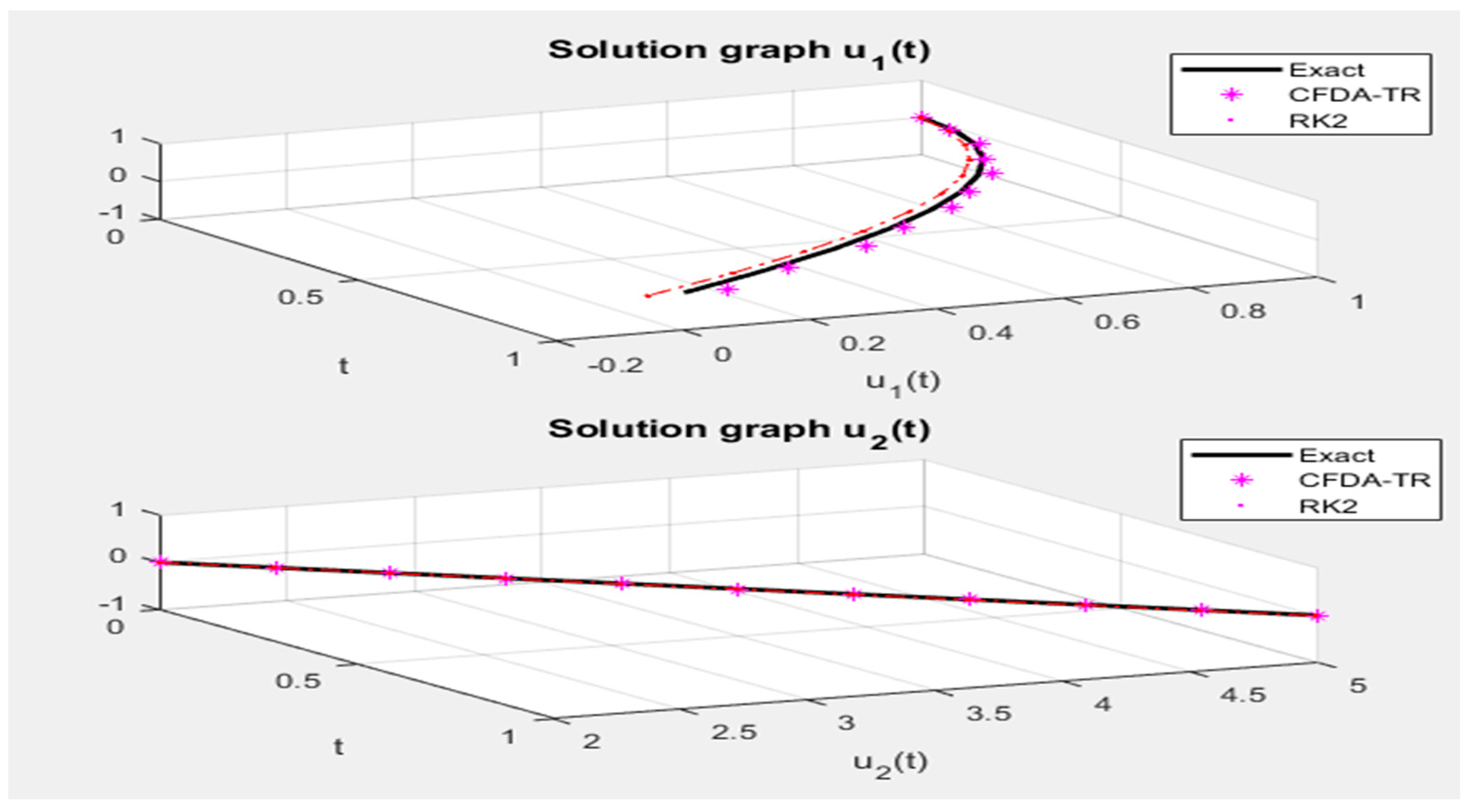
We can solve it by any numerical way, obtaining the ${\mathit{L}}_{\mathbf{1}}=\left[\begin{array}{cc}0.9842119511232& 2.30000733175\end{array}\right]$. We completed all the steps in the algorithm. Table 1 presents a comparison between the exact solution and the Runge–Kutta methods (RK2) in Reference [21], with the numerical solution of the central finite difference techniques via trapezoidal methods (a new method) for $u_1\left(t\right)$ and $u_2\left(t\right)$ depending on the least square error, see Table 1, Table 2 and Table 3 and Figure 1.

Table 1. A comparison between the exact solution with the RK2 method and the CFDA via TR.

${\mathit{t}}_{\mathit{r}}$	${\mathit{u}}_1\left(\mathit{t}\right)$			${\mathit{u}}_2\left(\mathit{t}\right)$
	Exact	RK2	New Method	Exact	RK2	New Method
$0.0$	$1.00$	$1.00$	$1.00$	$2.0$	$2.00$	$2.00$
$0.1$	$0.99$	$0.9810638182$	$0.9842119511$	$2.3$	$2.297486167$	$2.300007332$
$0.2$	$0.96$	$0.9444978611$	$0.9685499639$	$2.6$	$2.595284287$	$2.599965371$
$0.3$	$0.91$	$0.8891637088$	$0.9128294349$	$2.9$	$2.893243941$	$2.89998709$
$0.4$	$0.84$	$0.8144616925$	$0.8607297536$	$3.2$	$3.191332197$	$3.199909693$
$0.5$	$0.75$	$0.7200029143$	$0.7631618746$	$3.5$	$3.489569121$	$3.499846336$
$0.6$	$0.64$	$0.6054975247$	$0.6747355938$	$3.8$	$3.788012399$	$3.799529567$
$0.7$	$0.51$	$0.4707040816$	$0.5346474538$	$4.1$	$4.086751178$	$4.099139275$
$0.8$	$0.36$	$0.3154024787$	$0.4108090799$	$4.4$	$4.385901397$	$4.398272606$
$0.9$	$0.19$	$0.1393776737$	$0.2277729822$	$4.7$	$4.685599549$	$4.697312287$
$1.0$	$0.00$	$-0.057591078$	$0.0698805932$	$5.0$	$4.985992714$	$4.995629804$
${\left(L.S.E\right)}_{u_1}$		$0.129092$ $\times {10}^{-01}$	$0.114233$ $\times {10}^{-01}$	${\left(L.S.E\right)}_{u_2}$	$0.117972$ $\times {10}^{-02}$	$0.303016$ $\times {10}^{-04}$

Table 2. The mean least square error with running time is shown as a comparison between the RK2 and new methods.

Methods	RK2	New Method
${\left(L.S.E\right)}_U$	$0.704446\times {10}^{-02}$	$0.572679\times {10}^{-02}$
$R.Time/sec$	$0.129684$	$0.5619018$

Table 3. The mean least square errors and running times for RK2 and CFDA through TR with various choices of step size $h$.

	$\left(\mathit{N},\mathit{h}\right)$	$\left(10,0.1\right)$		$\left(50,0.02\right)$		$\left(100,0.01\right)$		$\left(500,0.002\right)$
Method		${\left(\mathit{L}.\mathit{S}.\mathit{E}\right)}_{\mathit{U}}$	$\mathit{R}.\mathit{T}/\mathit{s}\mathit{e}\mathit{c}$	${\left(\mathit{L}.\mathit{S}.\mathit{E}\right)}_{\mathit{U}}$	$\mathit{R}.\mathit{T}/\mathit{s}\mathit{e}\mathit{c}$	${\left(\mathit{L}.\mathit{S}.\mathit{E}\right)}_{\mathit{U}}$	$\mathit{R}.\mathit{T}/\mathit{s}\mathit{e}\mathit{c}$	${\left(\mathit{L}.\mathit{S}.\mathit{E}\right)}_{\mathit{U}}$	$\mathit{R}.\mathit{T}/\mathit{s}\mathit{e}\mathit{c}$
RK2		$0.704446$ $\times {10}^{-02}$	$0.129684$	$0.381939$ $\times {10}^{-03}$	$0.313021$	$0.141674$ $\times {10}^{-03}$	$0.856781$	$0.180299$ $\times {10}^{-04}$	$17.79277$
New Method		$0.572679$ $\times {10}^{-02}$	$0.5619018$	$0.284486$ $\times {10}^{-03}$	$0.6428377$	$0.8050076$ $\times {10}^{-04}$	$0.735199$	$0.3479825$ $\times {10}^{-05}$	$22.75923$

Figure 1. The numerical approximation of $\left[u_1\left(t\right),u_2\left(t\right)\right]$ by CFDA-TR and RK2 with the exact solution of Example 1.

Example 2.

Consider that a linear system of VI-FDEs for fractional multi-order lies in$\left(0,1\right)$on a closed, bounded interval$\left[0,1\right]:$

$$\begin{gathered} {}_0{}^{C}D_t^{0.6} u_1\left(t\right)+2{}_0{}^{C}D_t^{0.2} u_1\left(t\right)-u_1\left(t\right)=f_1\left(t\right)-{{\displaystyle \int }}_0^t\left[2\mathrm{s}{e}^t{u}_1\left(s\right)+\left(\frac{t}{2}-s\right)u_2\left(s\right)\right]ds \\ {}_0{}^{C}D_t^{0.5} u_2\left(t\right)+{}_0{}^{C}D_t^{0.4} u_2\left(t\right)-3u_2\left(t\right)=f_2\left(t\right)+{{\displaystyle \int }}_0^t\left[\left(s-\cos t\right)u_1\left(s\right)-ts{u}_2\left(s\right)\right]ds \end{gathered}$$

where

$$\begin{gathered} f_1\left(t\right)=\frac{2}{\mathsf{\Gamma }\left(1.4\right)}{t}^{0.4}+\frac{4}{\mathsf{\Gamma }\left(1.8\right)}{t}^{0.8}-2t+e^t\left(t-1\right)-\frac{1}{2}t\left(e^t-1\right)+\frac{1}{3}{t}^2{e}^t\left(4t+3\right) \\ {f}_2\left(t\right)=-\left(\sqrt{t}{E}_{1,1.5}\left(t\right)+\sqrt[5]{t^3}{E}_{1,1.6}\left(t\right)+3\right)+3e^t+t^2\left(\cos t-\frac{1}{2}\right)-t\left(e^t\left(t-1\right)+1\right)+t\cos t-\frac{1}{6}{t}^3 \end{gathered}$$

with initial conditions $u_1\left(0\right)=1 and u_2\left(0\right)=0$, the exact solutions are $u_1\left(t\right)=2t+1and{u}_2\left(t\right)=1-e^t$, where $E_{\alpha ,\beta }\left(t\right)$ is the Mittag–Leffler function of two parameters and is defined by $E_{\alpha ,\beta }\left(t\right)=\underset{N_0\to \infty }{\lim }{{\displaystyle \sum }}_{k=0}^{N_0}\frac{t^k}{\mathsf{Г}\left(\alpha k+\beta \right)}$ [3].

Take $N=10,h=0.1$, and $t_r=rh, r=0,1,2,\dots ,N$. From Equations (9), (10), (18), and (19), respectively, where $n=2$ and $m=2$ with ${\sigma }_{12}=0.6,{\sigma }_{11}=0.2,{\sigma }_{10}=0, {\sigma }_{22}=0.5,{\sigma }_{21}=0.4,{\sigma }_{20}=0$, $\left[a_{1\ell }\right]=\left[1,2,-1\right], \left[a_{2\ell }\right]=\left[1,1,-3\right],and \ell =0,1,2$, by running the MatLab program ASVIFT-C (0,1], we obtain:

$$\begin{array}{cc}\begin{array}{cc}\left(\begin{array}{c}{A}_n^{{\sigma }_1}(\ell )\\ A_n^{{\sigma }_2}(\ell )\end{array}\right)=\left(\begin{array}{cc}2.243454329& 1.701654293\\ 1.784124116& 1.405620191\end{array}\right)& ;\end{array}& \left(\begin{array}{c}{H}_n^{{\sigma }_1}\\ H_n^{{\sigma }_2}\end{array}\right)\end{array}=\left(\begin{array}{c}3.945108623\\ 3.189744307\end{array}\right)$$

and

$$\begin{array}{cc}\begin{array}{cc}\left(\begin{array}{c}{}_{}{}^{L}A_{n,1}^{{\sigma }_1}(\ell )\\ {}_{}{}^{L}A_{n,1}^{{\sigma }_2}(\ell )\end{array}\right)=\left(\begin{array}{cc}4.486908659& 3.403308586\\ 3.568248232& 2.811240382\end{array}\right)& ;\end{array}& \left(\begin{array}{c}{}_{}{}^{L}H_{n,1}^{{\sigma }_1}\\ {}_{}{}^{L}H_{n,1}^{{\sigma }_2}\end{array}\right)\end{array}=\left(\begin{array}{c}6.890217245\\ 3.379488614\end{array}\right)$$

For all $\ell =\overline{0:n-1}$. After applying step (3) in the ASVIFT-C algorithm, we obtain the linear system:

$$\left[G_1:W_1\right]=\left[\begin{array}{ccc}\begin{array}{cc}6.897585051& -0.000833333\\ 0.04641687493& 3.379821947\end{array}& \begin{array}{c}:\\ :\end{array}& \begin{array}{c}8.277189689\\ -0.3098033494\end{array}\end{array}\right]$$

We can solve it by any numerical way, obtaining the ${\mathit{L}}_{\mathbf{1}}=\left[\begin{array}{cc}1.199999639& -0.1081428514\end{array}\right]$. Then, complete all the steps in the algorithm. Table 4 presents and compares the exact solution with the numerical solution of central finite difference techniques via trapezoidal methods for $u_1\left(t\right)$ and $u_2\left(t\right)$ depending on the least square error and the mean least square error of the given system with running time, see Table 4 and Table 5 and Figure 2.

Table 4. A comparison of the exact solution with the numerical solution of CFDA via TR.

${\mathit{t}}_{\mathit{r}}$	${\mathit{u}}_1\left(\mathit{t}\right)$		${\mathit{u}}_2\left(\mathit{t}\right)$
	Exact	New Method	Exact	New Method
$0.0$	$1$	$1$	$0$	$0$
$0.1$	$1.2$	$1.19999963883$	$0.105170918076$	$0.108142851394$
0.2	$1.4$	$1.39976683352$	$0.22140275816$	$0.216175550843$.
$0.3$	$1.6$	$1.59955904788$	$0.349858807576$	$0.336507514037$
$0.4$	$1.8$	$1.79918472125$	$0.491824697641$	$0.464181398002$
$0.5$	$2.0$	$1.99883683551$	$0.6487212707$	$0.602529087892$
$0.6$	$2.2$	$2.19841309215$	$0.822118800391$	$0.750610102765$
$0.7$	$2.4$	$2.39809591718$	$1.01375270747$	$0.909592167453$
$0.8$	$2.6$	$2.5978823718$	$1.22554092849$	$1.07966470682$
$0.9$	$2.8$	$2.7979850329$	$1.45960311116$	$1.26171992117$
$1.0$	$3.0$	$2.99850160438$	$1.71828182846$	$1.45671629616$
${\left(L.S.E\right)}_{u_1}$		$0.1919988$ $\times {10}^{-04}$	${\left(L.S.E\right)}_{u_2}$	$0.14792935$ $\times {10}^{-00}$
${\left(L.S.E\right)}_U$		$0.7397427566\times {10}^{-01}$
$R.Time/sec$		$0.5701562$

Table 5. The mean least square errors and running times for CFDA through TR with various choices of step size $h$.

	$\left(\mathit{N},\mathit{h}\right)$	$\left(10,0.1\right)$		$\left(50,0.02\right)$		$\left(100,0.01\right)$		$\left(500,0.002\right)$
$\mathbf{Method}$		${\left(\mathit{L}.\mathit{S}.\mathit{E}\right)}_{\mathit{U}}$	$\mathit{R}.\mathit{T}/\mathit{s}\mathit{e}\mathit{c}$	${\left(\mathit{L}.\mathit{S}.\mathit{E}\right)}_{\mathit{U}}$	$\mathit{R}.\mathit{T}/\mathit{s}\mathit{e}\mathit{c}$	${\left(\mathit{L}.\mathit{S}.\mathit{E}\right)}_{\mathit{U}}$	$\mathit{R}.\mathit{T}/\mathit{s}\mathit{e}\mathit{c}$	${\left(\mathit{L}.\mathit{S}.\mathit{E}\right)}_{\mathit{U}}$	$\mathit{R}.\mathit{T}/\mathit{s}\mathit{e}\mathit{c}$
New Method		$0.7397428$ $\times {10}^{-01}$	$0.570156$	$0.8806996$ $\times {10}^{-02}$	$0.701179$	$0.2640132$ $\times {10}^{-02}$	$0.805054$	$0.12670067$ $\times {10}^{-03}$	$27.25336$

Figure 2. The numerical approximation of $\left[u_1\left(t\right),u_2\left(t\right)\right]$ by CFDA-TR with exact solution of Example 2.

Example 3.

Consider that a linear system of VI-FDEs for fractional multi-order lies in$\left(0,1\right)$on a closed, bounded interval$\left[0,1\right]$:

$$\begin{gathered} {}_0{}^{C}D_t^{0.9} u_1\left(t\right)-3u_1\left(t\right)=f_1\left(t\right)+{{\displaystyle \int }}_0^t\left[\mathrm{s}\ast \sin \left(t\right)u_1\left(s\right)+\left(2-st\right)u_2\left(s\right)-st{u}_3\left(s\right)\right]ds \\ {}_0{}^{C}D_t^{0.7} u_2\left(t\right)+u_2\left(t\right)=f_2\left(t\right)+{{\displaystyle \int }}_0^t\left[\left(s+2t\right)u_1\left(s\right)+s{e}^t{u}_2\left(s\right)+\left(s+t\right)u_3\left(s\right)\right] ds \\ {}_0{}^{C}D_t^{0.2} u_3\left(t\right)-\frac{1}{2}{u}_3\left(t\right)=f_3\left(t\right)+{{\displaystyle \int }}_0^t\left[\left(t^2-s+1\right)u_1\left(s\right)+\left(s-e^t\right)u_2\left(s\right)+\left(2t-s\right)s u_3\left(s\right)\right]ds) \end{gathered}$$

where

$$\begin{gathered} f_1\left(t\right)=\frac{1}{\mathsf{\Gamma }\left(1.1\right)}{t}^{0.1}-\frac{1}{10}t\left(2t^5-5t^3+5t^2-20\right)-\frac{1}{6}{t}^3\left(4t-3\right)-\frac{1}{6}{t}^2\sin \left(t\right)\left(2t+3\right)-3t-3 \\ {f}_2\left(t\right)=\frac{6}{\mathsf{\Gamma }\left(3.3\right)}{t}^{2.3}+\frac{1}{6}{t}^2\left(10t-9\right)-\frac{1}{6}{t}^2\left(8t+15\right)-\frac{1}{10}{t}^2{e}^t\left(2t^3+5\right)+t^3+1 \\ {f}_3\left(t\right)=\frac{-2}{\mathsf{\Gamma }\left(1.8\right)}{t}^{0.8}-\frac{1}{60}t\left(120t-60e^t-15t^3{e}^t-40t^2+30t^3+12t^4+60\right)+t-\frac{1}{2} \end{gathered}$$

together with the initial conditions $u_1\left(0\right)=u_2\left(0\right)=u_3\left(0\right)=1$, while the exact solutions are $u_1\left(t\right)=t+1,u_2\left(t\right)=1+t^3, and{u}_3\left(t\right)=1-2t$.

From Equations (9), (10), (18), and (19), respectively, where $n=1$ and $m=3$ with ${\sigma }_{11}=0.9,{\sigma }_{10}=0, {\sigma }_{21}=0.7,{\sigma }_{20}=0$, ${\sigma }_{31}=0.2, and {\sigma }_{30}=0$ and the constant coefficients are $\left[a_{1\ell }\right]=\left[1,-3\right], \left[a_{2\ell }\right]=\left[1,1\right], \left[a_{3\ell }\right]=\left[1,-\frac{1}{2}\right], and \ell =0,1,$ by running the MatLab program of algorithm ASVIFT-C (0,1] with a fixed $N=10,h=0.1,$ $t_r=rh,and r=0,1,2,\dots ,N,$ we obtain:

$$\begin{array}{cc}\begin{array}{cc}\left(\begin{array}{c}\begin{array}{c}{A}_n^{{\sigma }_1}(\ell )\\ A_n^{{\sigma }_2}(\ell )\end{array}\\ A_n^{{\sigma }_3}(\ell )\end{array}\right)& =\end{array}& \left(\begin{array}{c}\begin{array}{c}{H}_n^{{\sigma }_1}\\ H_n^{{\sigma }_2}\end{array}\\ H_n^{{\sigma }_3}\end{array}\right)\end{array}=\left(\begin{array}{c}4.174739013\\ 2.792220602\\ 0.8508271466\end{array}\right)$$

and

$$\begin{array}{cc}\begin{array}{cc}\left(\begin{array}{c}\begin{array}{c}{}_{}{}^{L}A_{n,1}^{{\sigma }_1}(\ell )\\ {}_{}{}^{L}A_{n,1}^{{\sigma }_2}(\ell )\end{array}\\ {}_{}{}^{L}A_{n,1}^{{\sigma }_3}(\ell )\end{array}\right)=\left(\begin{array}{c}8.349478025\\ 5.584441204\\ 1.701654293\end{array}\right)& ;\end{array}& \left(\begin{array}{c}\begin{array}{c}{}_{}{}^{L}H_{n,1}^{{\sigma }_1}\\ {}_{}{}^{L}H_{n,1}^{{\sigma }_2}\end{array}\\ {}_{}{}^{L}H_{n,1}^{{\sigma }_3}\end{array}\right)\end{array}=\left(\begin{array}{c}5.349478025\\ 6.584441204\\ 1.201654293\end{array}\right)$$

For $\ell =\overline{0:n-1}$. After applying step (3) in the ASVIFT-C algorithm, we obtain the linear system:

$$\left[G_1:W_1\right]=\left[\begin{array}{ccc}\begin{array}{ccc}5.349145247& -0.09966666667& 0.0003333333333\\ -0.01333333333& 6.580757301& -0.008333333333\\ -0.04716666667& 0.05192521257& 1.194987626\end{array}& \begin{array}{c}\begin{array}{c}:\\ :\end{array}\\ :\end{array}& \begin{array}{c}5.784609972\\ 6.571627994\\ 0.9560576097\end{array}\end{array}\right]$$

We can solve it by any numerical way, obtaining the ${\mathit{L}}_{\mathbf{1}}=\left[\begin{array}{ccc}1.100025247& 1.001854479& 0.799941862\end{array}\right]$. Then, complete all the steps in the algorithm. Table 6 presents and compares the correct solution to the numerical solution of central finite difference techniques via trapezoidal methods for $u_1\left(t\right)$, $u_2\left(t\right),$ and $u_3\left(t\right)$ depending on the least square error and the mean least square error of the given system with running time, see Table 6 and Table 7 and Figure 3.

Table 6. A comparison of the correct solution to the numerical solution of central finite difference approaches CFDA via trapezoidal method.

${\mathit{t}}_{\mathit{r}}$	${\mathit{u}}_1\left(\mathit{t}\right)$		${\mathit{u}}_2\left(\mathit{t}\right)$		${\mathit{u}}_3\left(\mathit{t}\right)$
	Exact	New Method	Exact	New Method	Exact	New Method
$0.0$	$1.0$	$1.0$	$1.0$	$1.0$	$1.0$	$1.0$
$0.1$	$1.1$	$1.1000252469$	$1.001$	$1.0018544793$	$0.8$	$0.79994186203$
$0.2$	$1.2$	$1.200062393$	$1.008$	$1.0036504727$	$0.6$	$0.6000833090$
$0.3$	$1.3$	$1.3000985204$	$1.027$	$1.0222104148$	$0.4$	$0.40036111198$
$0.4$	$1.4$	$1.4000621925$	$1.064$	$1.0501005888$	$0.2$	$0.2010432399$
$0.5$	$1.5$	$1.499814675$	$1.125$	$1.109723168$	$0.0$	$0.002415649$
$0.6$	$1.6$	$1.5991872543$	$1.216$	$1.186976334$	$-0.2$	$-0.195143098$
$0.7$	$1.7$	$1.6978607045$	$1.343$	$1.3123337772$	$-0.4$	$-0.3909495187$.
$0.8$	$1.8$	$1.7954625075$	$1.512$	$1.461637942$	$-0.6$	$-0.584276051$
$0.9$	$1.9$	$1.8913367143$	$1.729$	$1.6773103413$	$-0.8$	$-0.773729972$
$1.0$	$2.0$	$1.9846294819$	$2.0$	$1.9201550898$	$-1.0$	$-0.957862804$
${\left(L.S.E\right)}_{u_1}$		$0.33718378$ $\times {10}^{-03}$	${\left(L.S.E\right)}_{u_2}$	$0.13835322$ $\times {10}^{-01}$	${\left(L.S.E\right)}_{u_3}$	$0.2825465$ $\times {10}^{-02}$
${\left(L.S.E\right)}_U$		$0.5665990261\times {10}^{-02}$
$R.Time/sec$		0.8356171

Table 7. The least square errors and running times for CFDA using the TR for various choices of step size $h$ are listed.

	$\left(\mathit{N},\mathit{h}\right)$	$\left(10,0.1\right)$		$\left(50,0.02\right)$		$\left(100,0.01\right)$		$\left(500,0.002\right)$
$\mathbf{Method}$		${\left(\mathit{L}.\mathit{S}.\mathit{E}\right)}_{\mathit{U}}$	$\mathit{R}.\mathit{T}/\mathit{s}\mathit{e}\mathit{c}$	${\left(\mathit{L}.\mathit{S}.\mathit{E}\right)}_{\mathit{U}}$	$\mathit{R}.\mathit{T}/\mathit{s}\mathit{e}\mathit{c}$	${\left(\mathit{L}.\mathit{S}.\mathit{E}\right)}_{\mathit{U}}$	$\mathit{R}.\mathit{T}/\mathit{s}\mathit{e}\mathit{c}$	${\left(\mathit{L}.\mathit{S}.\mathit{E}\right)}_{\mathit{U}}$	$\mathit{R}.\mathit{T}/\mathit{s}\mathit{e}\mathit{c}$
New Method		$0.5665990$ $\times {10}^{-02}$	0.835617	$0.3657621$ $\times {10}^{-03}$	$0.92613$	$0.1063399$ $\times {10}^{-03}$	$10.8314$	$0.5304612$ $\times {10}^{-05}$	38.8658

Figure 3. The numerical approximation of $\left[u_1\left(t\right),u_2\left(t\right),u_3\left(t\right)\right]$ by CFDA-TR with exact solution of Example 3.

8. Discussion

This paper presents an improved, new numerical scheme for approximating the solution of LSVI-FDEs with constant coefficients including trapezoidal rules using a central finite difference approach (CFDA) for a Caputo derivative sense. The explicit numerical technique for LSVI-FDEs was explored in terms of error analysis, stability, and convergence, finally stating the important theorems of it. A computer program was built in MatLab for the new algorithm ASVIFT-C, and three test examples were given to confirm the computational validity and numerical accuracy.

I concluded the following points after comparing the accuracy and speed of computing. The least square error and running time are also presented in tabular form.

(1)

The ASVIFT-C scheme is more accurate and better than the Runge–Kutta method (RK2) when step sizes are equal.

(2)

The convergence order of each fractional part is $O\left(h^{3-{\sigma }_{1n}}\right)$; $n$ is the number of terms and ${\sigma }_{1n}\in \left(0,1\right]$. Thus, systems (1) and (2) are convergent and conditionally stable (see theorems 9 and 10).

(3)

The precision of the results was determined by the technique used and the step length $h$, which reduced as $h$ decreased, i.e., as the number of mesh points increased, $N$. See the Table 8 below, for further information.

Table 8. Central Finite Difference Approaches (CFDA) via TRAPEZOIDAL Methods (TR) for difference examples for increasing N:.

Central Finite Difference Approaches (CFDA) via TRAPEZOIDAL Methods (TR)
Numbers of Points	$\mathit{N}=1000$		$\mathit{N}=\mathrm{10,000}$		$\mathit{N}=\mathrm{20,000}$		$\mathit{N}=\mathrm{30,000}$
Examples	${\left(\mathit{L}.\mathit{S}.\mathit{E}\right)}_{\mathit{U}}$	$\mathit{R}.\mathit{T}/\mathit{s}\mathit{e}\mathit{c}$	${\left(\mathit{L}.\mathit{S}.\mathit{E}\right)}_{\mathit{U}}$	$\mathit{R}.\mathit{T}/\mathit{s}\mathit{e}\mathit{c}$	${\left(\mathit{L}.\mathit{S}.\mathit{E}\right)}_{\mathit{U}}$	$\mathit{R}.\mathit{T}/\mathit{s}\mathit{e}\mathit{c}$	${\left(\mathit{L}.\mathit{S}.\mathit{E}\right)}_{\mathit{U}}$	$\mathit{R}.\mathit{T}/\mathit{s}\mathit{e}\mathit{c}$
Example 1	$0.901382$$\times {10}^{-6}$	$6.282154$	$0.100498$$\times {10}^{-7}$	$431.6251$	$0.258596$$\times {10}^{-8}$	$1673.323$	$0.11678$$\times {10}^{-8}$	$3732.363$
Example 2	$0.326878$$\times {10}^{-4}$	$6.802216$	$0.34047$$\times {10}^{-6}$	416.0578	$0.854885$$\times {10}^{-7}$	$1548.502$	$0.38064$$\times {10}^{-7}$	$3619.319$
Example 3	$0.1413059$$\times {10}^{-5}$	$12.56362$	$0.1763703$$\times {10}^{-7}$	$1059.3332$	$0.1160868$$\times {10}^{-7}$	$4228.4249$	$0.754437$$\times {10}^{-8}$	$9517.801$

(4)

The numerical experiments showed that the CFDA-TR is the most popular method that gives the best approximation to the exact solution among the methods and performs extremely well, especially for small step sizes.

This new difference scheme can be applied to many other systems involving the Caputo fractional derivative. In future work, I will consider the stability and error estimates for the proposed numerical method to solve LSVI-FDEs applying Simpson and Midpoints via CFDA.

References

1. Podldubny, I. Fractional Differential Equation; Academic Press: San Diego, CA, USA, 1999. [Google Scholar]
2. Podlubny, I. Geometric and Physical Interpretation of Fractional Integral and Fractional Differentiation. J. Fract. Calc. Appl. Anal. 2002, 5, 367–386. [Google Scholar]
3. Samko, S.G.; Kilbas, A.A.; Marichev, O.I. Fractional Integrals and Derivatives: Theory and Applications; Gordon and Breach Science Publishers: Philadelphia, PA, USA, 1993. [Google Scholar]
4. Kilbas, A.A.; Srivastava, H.M.; Trujillo, J.J. Theory and Applications of Fractional Differential Equations; Elsevier: Amsterdam, The Netherlands, 2006. [Google Scholar]
5. Sabatier, J.; Agrawal, O.P.; Machado, J.A.T. Advances in Fractional Calculus: Theoretical Developments and Applications in Physics and Engineering; Beijing World Publishing Corporation: Beijing, China, 2014. [Google Scholar]
6. Erturk, V.S.; Kumar, P. Solution of a COVID-19 model via new generalized Caputo-type fractional derivatives. Chaos Solitons Fractals 2020, 139, 110280. [Google Scholar] [CrossRef] [PubMed]
7. Iomin, A. Fox H-Functions in Self-Consistent Description of a Free-Electron Laser. Fractal Fract. 2021, 5, 263. [Google Scholar] [CrossRef]
8. Baleanu, D.; Jajarmi, A.; Asad, J.H.; Blaszczyk, T. The Motion of a Bead Sliding on a Wire in Fractional Sense. Acta Phys. Pol. A 2017, 131, 1561–1564. [Google Scholar] [CrossRef]
9. Baleanu, D.; Jajarmi, A.; Mohammadi, H.; Rezapour, S. A new study on the mathematical modelling of human liver with Caputo-Fabrizio fractional derivative. Chaos Soliton. Fractals 2020, 134, 109705. [Google Scholar] [CrossRef]
10. Baleanu, D.; Sajjadi, S.S.; Jajarmi, A.; Defterli, O.; Asad, J.H. The fractional dynamics of a linear triatomic molecule. Rom. Rep. Phys. 2021, 73, 105. [Google Scholar]
11. AL-Nasir, R.H. Numerical Solution of Volterra Integral Equations of the Second Kind. Master’s Thesis, Technology University, Baghdad, Iraq, September 1999. [Google Scholar]
12. AL-Rawi, S.N. Numerical Solution of First Kind Integral Equations of Convolutions Type. Master’s Thesis, Technology University, Baghdad, Iraq, 1995. [Google Scholar]
13. Saadati, R.; Raftari, B.; Adibi, H.; Vaezpour, S.M.; Shakeri, S. A Comparison Between the variational Iteration Method and Trapezoidal Rule for Solving Linear Integro Differential Equations. World Appl. Sci. J. 2008, 4, 321–325. [Google Scholar]
14. AL-Jawary, M.A.W. Numerical Methods for System of Integral Equations. Master’s Thesis, Baghdad University, Baghdad, Iraq, 2005. [Google Scholar]
15. AL-Dahan, O.K. Approximated Solution of Volterra Integral Equation. Master’s Thesis, Technology University, Baghdad, Iraq, 1996. [Google Scholar]
16. Ahmed, S.S.; Hamasalih, S.A. Numerical Treatment of the Most General Linear Volterra Integro-Fractional Differential Equations with Caputo Derivatives by Quadrature Methods. J. Math. Comput. Sci. 2012, 2, 1293–1311. [Google Scholar]
17. Shen, S.; Liu, F. Error analysis of an explicit finite difference approximation for the space fractional diffusion equation with insulated ends. ANZIAM J. 2005, 46, 871–887. [Google Scholar] [CrossRef] [Green Version]
18. Liu, F.; Zhuang, P.; Anh, V.; Turner, I. A fractional-order implicit difference approximation for the space-time fractional diffusion equation. ANZIAM J. 2006, 47, 48–68. [Google Scholar] [CrossRef] [Green Version]
19. Ahmed, S.S.; Mohammed Faeq, S.J. Bessel Collocation Method for Solving Fredholm & ndash; Volterra Integro-Fractional Differential Equations of Multi-High Order in the Caputo Sense. Symmetry 2021, 13, 2354. [Google Scholar] [CrossRef]
20. Ahmed, S.S.; Saeed, B.A. He’s homotopy perturbation method with modification for solving multi-higher nonlinear Fredholm integro-differential equations of fractional order. AIP Conf. Proc. 2019, 2096, 020010. [Google Scholar]
21. Ahmed, S.S. On System of Linear Volterra Integro-Fractional Differential Equations. Ph.D. Thesis, Sulaimani University, Sulaymaniyah, Iraq, 2009. [Google Scholar]
22. Oldham, K.; Spanier, J. The Fractional Calculus: Theory and Applications of Differentiation and Integration to Arbitrary Order; Academic Press, Inc.: Cambridge, MA, USA, 1974. [Google Scholar]
23. Weilbeer, M. Efficient Numerical Methods for Fractional Differential Equations and their analytical Background. US Army Med. Res. Mater. Command (Supported by the US Army Medical Research and Material Command Grant No. DAMD-17-01-1-0673 to the Cleveland Clinic- NASA Technical Rep.). 2005. Available online: https://d-nb.info/980333385/34 (accessed on 9 March 2022).
24. Burden, R.L.; Faires, J.D.; Burden, A.M. Numerical Analysis, 10th ed.; Publisher Cengage Learning: Boston, MA, USA, 2016. [Google Scholar]
25. Zamani, M. Three Simple Spline Method for Approximation and Interpolation of Data. Contemp. Eng. Sci. 2009, 2, 373–381. [Google Scholar]
26. Jwamer, K.H.; Ahmed, S.S.; Abdullah, D.K. Numerical Treatment Solution of Volterra Integro-Fractional Differential Equation by Using Linear Spline Function. J. Zankoy Sulaimani 2020, 22, 327–338. [Google Scholar] [CrossRef]
27. Dash, R.B.; Das, D. A Mixed Quadrature Rule by Blending Clenshaw-Curtis and Gauss-Legendre Quadrature Rules for Approximation of Real Definite Integrals in Adaptive. J. Comput. Math. Sci. 2012, 3, 131–247. [Google Scholar]
28. Marcus, M.; Minc, H. A Survey of Matrix Theory and Matrix Inequalities; Allyw and Bacon, Inc.: Boston, MA, USA, 1964. [Google Scholar]
29. Atkinson, K.E. An Introduction to Numerical Analysis, 2nd ed.; John Wiley & Sons, Inc.: Hoboken, NJ, USA, 1989. [Google Scholar]
30. Trefethen, L.N. Finite Difference and Spectral Methods for Ordinary and Partial Differential Equations; Cornell University: Ithaca, NY, USA, 1996. [Google Scholar]
31. Linz, P. Analytical and Numerical Methods for Volterra Equations; Siam: Philadelphia, PA, USA, 1985. [Google Scholar]
Figure 1. The numerical approximation of [ u 1 ( t ) , u 2 ( t ) ] by CFDA-TR and RK2 with the exact solution of Example 1.
Symmetry 14 00575 g001
Figure 2. The numerical approximation of [ u 1 ( t ) , u 2 ( t ) ] by CFDA-TR with exact solution of Example 2.
Symmetry 14 00575 g002
Figure 3. The numerical approximation of [ u 1 ( t ) , u 2 ( t ) , u 3 ( t ) ] by CFDA-TR with exact solution of Example 3.
Symmetry 14 00575 g003