Dynamic Performances of Technological Vibrating Machines

Abstract

Based on the research carried out within the Research Institute for Construction Equipment and Technology—ICECON S.A. Bucharest, consisting of the design and development of vibrating-action machines and of the technical analysis of optimization of the technological processes with vibrating equipment for highway construction works in Romania. Moreover, the physical and mathematical modeling of this mechanical system used the data obtained in the activity of the certification of the technical level of capability of the processing equipment in industry and construction, taking into account the provisions of procedures and regulations legally enforced by normative documents. These are based on a parametric analysis of the dynamics of the technological processing vibratory equipment and machines. Thus, both the evaluation method and the parametric optimization procedure were established. In this context, this paper presents a numerical analytical approach with discrete and continuous parametric variations, from where favorable areas of operation can be established. In this way, the optimization criteria in stabilized harmonic vibration regimes are approached based on the assessment of the vibration amplitude, of the force transmitted to the processed material and of the energy dissipated in the system. The presented dynamic model as well as the specific parameters were used in the design and/or numerical and experimental assessment for vibrating rammers with the amplitude of the perturbing force from 2 kN up to 100 kN, vibrating compactors with the amplitude of the perturbing force from 100 kN up to 200 kN and vibrating sieves for mineral aggregates with surface sieves of 6, 12 and 18 sqm. The symmetry/asymmetry properties are specific to the dynamic response in steady-state technological regime. Thus, the amplitude of vibrations in resonance presents asymmetry through a functional level necessary for the technological regime. The maximum force transmitted in the technological process is asymmetric in relation to the variation of the excitation pulsation; also, the dissipated energy has asymmetries in the postresonance. Hysteresis loops are symmetrical to the main axis. The originality of the research results comes from the establishment of dynamic parameters for the amplitude of technological vibration, the force transmitted to the working part, the energy dissipated on the cycle, hysteresis loops in a steady-state regime with digital display to identify the dynamic regime and the damping in the system. The calculation relations are specific to machines with a vibrating action and, on their basis, the vibrating equipment from Romania were designed, manufactured and tested, as mentioned in this paper.

1. Introduction

The technological capability of machines with a vibrating action is defined by the set of dynamic parameters necessary to ensure the established level of performance. The level of performance for the vibrating machines, according to the technological process it determines, is established either in normative documents (according to approved legal provisions) or via commercial means as a requirement from the beneficiary of the technology towards the machine manufacturer. The parameters of the dynamic models and the performances of the technological vibrations are finalized according to the functional particularities of the vibrating equipment [1,2].

The most common technologies where vibrating machines have a decisive role in ensuring the quality of material processing are the following:

(a)

sorting of granular and powdery materials for process industries (chemical, construction materials, pharmaceutical) [3,4];

(b)

transport and dosing of granular and pulverulent materials in the cement industry, construction materials, mining, preparation of concrete and asphalt mixtures, processing of mineral aggregates of gravel (river) and quarry [5,6];

(c)

realization of the technological processes in construction for dynamic sticking of the piles in the field, compaction by vibrations of road structures, the vibro-compaction of freshly poured concrete [7,8,9].

In Romania, dynamic equipment for construction were designed and developed, in which models and dynamic calculation relations were used and the authors of this article had a decisive role. Thus, the following vibrating action machines were designed, made, tested and approved: AVP1, AVP2, AVPP vibrating rammers in Timișoara; CVA 4–5, CVA 10 and CVA 20 vibrating compacting rollers in Iași; 6, 12 and18 sqm vibrating sieves with a number of 2–4 sieves for granules of 0–4 mm, 4–8 mm, 8–16 mm and 16–31 mm in Baia-Mare; vibratory conveyors and dosing machines of granular and powdery materials with mass flows of 2 up to 20 t/h in Sibiu and Brașov; vertical helical conveyors with dosing masses of 100 up to 500 kg/h in Pitești, Brașov [10,11,12,13].

For the above vibrating machines, the same dynamic diagram of a linear system with a degree of freedom—1DOF—which describes the functional behavior with a high level of confidence is valid. Thus, for all categories of vibratory machines for the specified technologies, the same linear dynamic model shall be used, based on which the defining parameters shall be established, namely: amplitude, transmitted force, degree of dynamic isolation and the dissipated energy with the representation of the hysteresis loop in steady-state vibration regime. The disruptive force is generated by eccentric masses m0 arranged at distance r versus the axis of rotation for the specified ω angular speed.

In essence, the inertial character of the dynamic response is drawn from the fact that the calculation model is provided with the concentrated (punctiform) mass of the perturbed material system with a harmonic perturbing force $F\left(t\right)=F_{0}sin\left(\omega t\right)$, where $F_0$ is the amplitude of the force and $\omega$ is the excitation pulsation. The amplitude of the perturbating force is variable depending on ω, expressed as $F_0=m_{0}r{\omega }^2$, where $m_{0}r$ is the static moment of the dynamic imbalance [14,15,16].

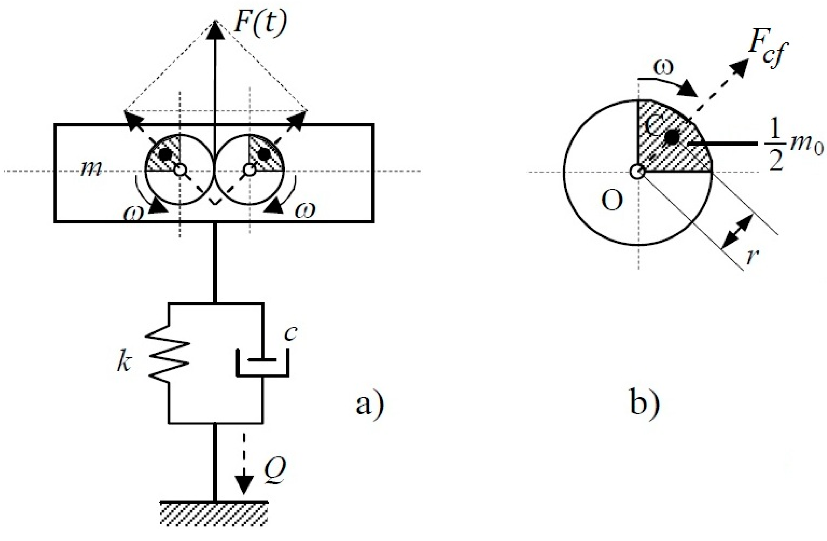
2. Dynamic Calculation Model

The Voigt–Kelvin viscoelastic linear dynamic system is characterized by structural constituent elements, namely: $m$—mass, $k$—coefficient of equivalent stiffness, $c$—coefficient of equivalent viscous amortization. In this case, the system can also be symbolized as MKC, that is mass m, stiffness k, damping c [1,2,14,15].

The harmonic excitation of the system is controlled by generating the dynamic external force applied to the center of gravity of the dynamic system. The applied harmonic dynamic force is $F=F\left(t\right)=F_{0}sin\left(\omega t\right)$, also known as disturbing/perturbating force, where $\omega$ is the pulsation of the excitation. The disturbing force in this case is $F=m_{0}r{\omega }^{2}sin\left(\omega t\right)$, with the system model shown in Figure 1; the inertial excitation is generated by the opposite symmetric rotational motion of the imbalanced masses with the centrifugal inertia forces $F_{cf}=\frac{1}{2}{m}_{0}r{\omega }^2$ and the vertical resultant amplitude $F_0=m_{0}r{\omega }^2$.

The analysis of the unidirectional motion, as a result of the perturbative force $F\left(t\right)$ with vertical direction of action, is performed by the coordinate $x=x\left(t\right)$ specific to the system with a single degree of freedom [6,10,17].

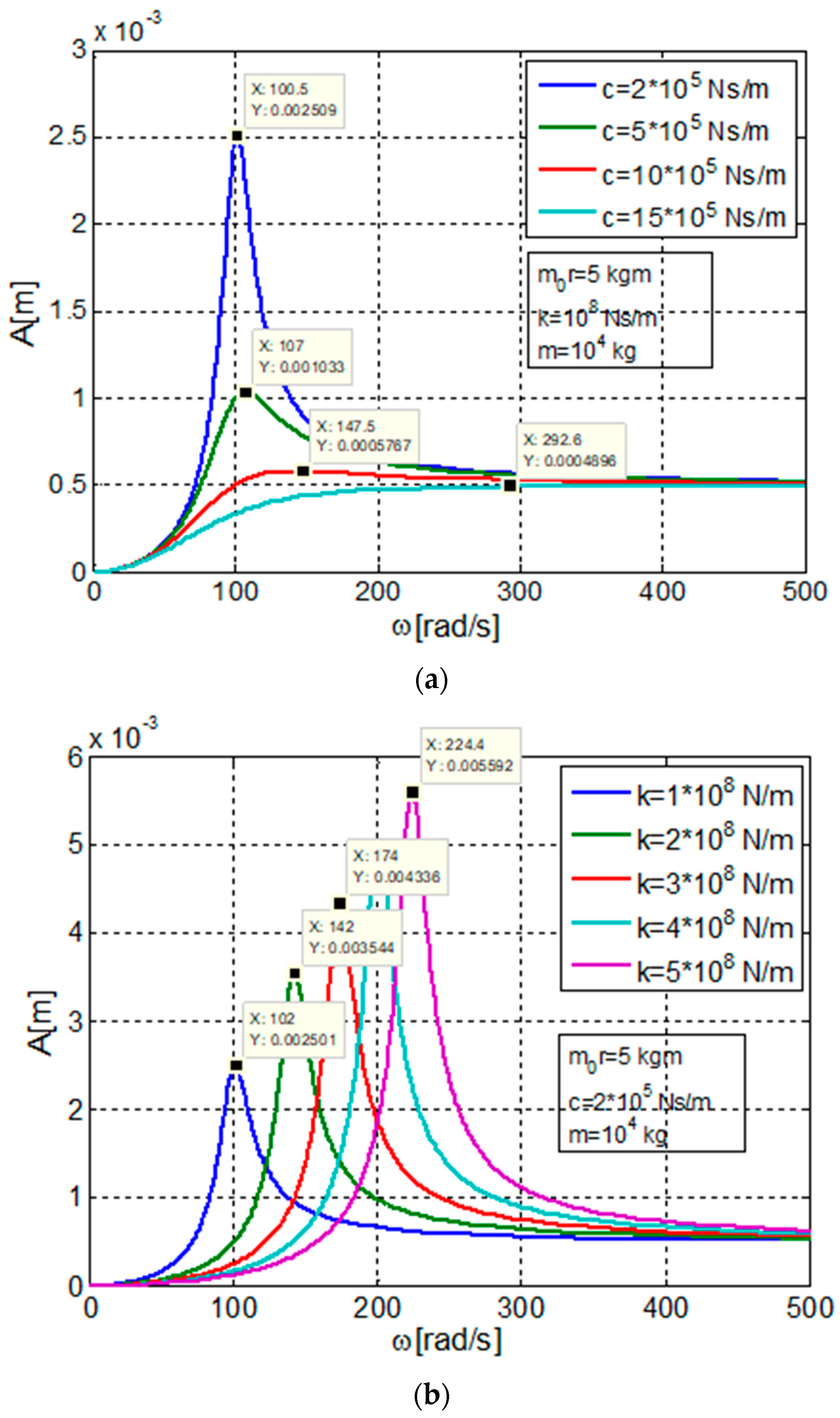
2.1. Dynamic Response of 1DOF System

In case of an excitation in force, the dynamic response is sought as an instantaneous displacement adequate rule, as $x=x\left(t\right)$ [18,19,20].

The instantaneous dynamic balance is given by the linear differential equation as:

$$m\ddot{x}+c\dot{x}+kx=F_0\mathit{sin}\omega t$$

(1)

It considers the complex function $\tilde{x}={\tilde{X}}_0{e}^{j\omega t}$, in which ${\tilde{X}}_0=A{e}^{-j\phi }$, where $\phi$ is the phase difference between the instantaneous displacement $x=x\left(t\right)$ and the harmonic perturbing force $F\left(t\right)=F_{0}sin\left(\omega t\right)$. In this case, $x=Re\tilde{x}$, where $\tilde{x}={\tilde{X}}_0{e}^{j\omega t}$, with ${\tilde{X}}_0=A{e}^{j\phi }$, and $\tilde{F}\left(t\right)=\tilde{F}=F_0{e}^{j\omega t}$, which enables the transposition of the Equation (1) in complex formulation, as follows:

$$m\ddot{\tilde{x}}+c\dot{\tilde{x}}+k\tilde{x}=\tilde{F}\left(t\right)$$

(2)

The derivates $\ddot{\tilde{x}}$ and $\dot{\tilde{x}}$ of coordinate $\tilde{x}$ are:

$$\dot{\tilde{x}}=j\omega {\tilde{X}}_0{e}^{j\omega t}=j\omega \tilde{x}$$

$$\ddot{\tilde{x}}=-{\omega }^2{\tilde{X}}_0{e}^{j\omega t}=-{\omega }^2\tilde{x}$$

which replaced in (2), leads to:

$$-m{\omega }^2\tilde{x}+jc\omega \tilde{x}+k\tilde{x}=F_0{e}^{j\omega t}$$

or

$$\tilde{x}=\frac{1}{\left(k-m{\omega }^2\right)+jc\omega }{F}_0{e}^{j\omega t}={\tilde{X}}_0{e}^{j\omega t},$$

(3)

from where results:

$${\tilde{X}}_0=F_0\frac{1}{\left(k-m{\omega }^2\right)+jc\omega }$$

or

$${\tilde{X}}_0=A{e}^{j\phi }=F_0\frac{k-m{\omega }^2}{D}-j{F}_0\frac{c\omega }{D}$$

where

$$D={\left(k-m{\omega }^2\right)}^2+c^2{\omega }^2$$

$\left|{\tilde{X}}_0\right|$, the module of ${\tilde{X}}_0$, results from the relation (3), as follows:

$${\left|{\tilde{\mathit{X}}}_{\mathbf{0}}\right|}^{\mathbf{2}}={\mathit{A}}^{\mathbf{2}}={\mathit{F}}_{\mathbf{0}}{}^{\mathbf{2}}\frac{{\left(\mathit{k}-\mathit{m}{\omega }^{\mathbf{2}}\right)}^{\mathbf{2}}+{\mathit{c}}^{\mathbf{2}}{\mathbf{\omega }}^{\mathbf{2}}}{{\mathit{D}}^{\mathbf{2}}}={\mathit{F}}_{\mathbf{0}}{}^{\mathbf{2}}\frac{\mathit{D}}{{\mathit{D}}^{\mathbf{2}}}$$

or

$$\left|{\tilde{X}}_0\right|=A=F_0\frac{1}{\sqrt{{\left(k-m{\omega }^2\right)}^2+c^2{\omega }^2}}$$

(4)

The instantaneous movement law or the instantaneous coordinate $x\left(t\right)=x$ can be expressed as:

$$x\left(t\right)=x=Asin\left(\omega t-\phi \right)$$

(5)

Phase $\phi$ results from relation (3) as follows:

$$A\left(cos\phi +jsin\phi \right)=\frac{F_0}{D}\left(k-m{\omega }^2\right)-j\frac{F_0}{D}c\omega$$

from where, we have

$$\{\begin{array}{c}Acos\phi =\frac{F_0}{D}\left(k-m{\omega }^2\right)\\ Asin\phi =-\frac{F_0}{D}c\omega \end{array}$$

(6)

and the phase is:

$$tan\phi =-\frac{c\mathbf{\omega }}{k-m{\mathbf{\omega }}^2}\mathbf{\to }\phi =arctan\left(-\frac{c\mathbf{\omega }}{k-m{\mathbf{\omega }}^2}\right)$$

(7)

Amplitude $A$ of the instantaneous displacement and the phase $\phi$ can be expressed function of the non-dimensional quantities, as follows:

(a)

$\mathsf{\Omega }=\frac{\omega }{{\omega }_{\mathit{n}}}$-relative pulsation;

(b)

$\mathbf{\zeta }=\frac{\mathit{c}}{\mathbf{2}\mathit{m}{\omega }_{\mathit{n}}}$–the fraction of the critical amortization specific to the linear viscous-elastic systems with discrete viscous dissipators, characterized by the viscous amortization coefficient c.

The math relation between $\zeta$ and $\mathsf{\Omega }$ is $\frac{c\omega }{k}=2\zeta \mathsf{\Omega }$.

The amplitude in relation (4) can be written

$$A\left(\zeta ,\mathsf{\Omega }\right)=\frac{F_0}{k}\frac{1}{\sqrt{{\left(1-{\mathsf{\Omega }}^2\right)}^2+{\left(2\zeta \mathsf{\Omega }\right)}^2}}$$

(8)

and the phase in relation (7) can be written as follows:

$$tan\phi =-\frac{c\mathbf{\omega }}{k}\frac{1}{1-\frac{m{\mathbf{\omega }}^2}{k}}$$

or

$$tan\phi =-\frac{2\zeta \mathsf{\Omega }}{1-{\mathsf{\Omega }}^2}$$

(9)

The harmonic dynamic response in instantaneous displacement $x=x\left(t\right)$ is:

$$x=x\left(t\right)=Asin\left(\mathbf{\omega }t+\phi \right)$$

The dynamic regime for a mechanical system with discrete variation of the damping and of the stiffness may be represented by the variation of amplitude A in relation with the current variant ω function of the discrete variation of damping coeff c and stiffness k (Figure 2) [21,22,23].

Figure 2a shows that, for constant stiffness c, at four discrete/different values of damping c, the dynamic system is stable and without significant influences of damping variation when the operating mode is in postresonance regime, with pulsation values $\omega \ge 300\mathrm{rad}/\mathrm{s}$.

Figure 2b shows that, for constant damping coefficient c, the discrete variation of the stiffness k leads to the resonance points at discrete values of the pulsation ω. The maximum values of the forced steady-state vibration amplitude are on the straight line described by the equation $A\left(\omega \right)=0.07483+0.02525\omega \left[\times {10}^{-3}\mathrm{m}\right]$ (for $\omega >100 \mathrm{rad}/\mathrm{s}$). These points of maximum amplitude characterize the phenomenon of amplitude resonance of the dynamic system.

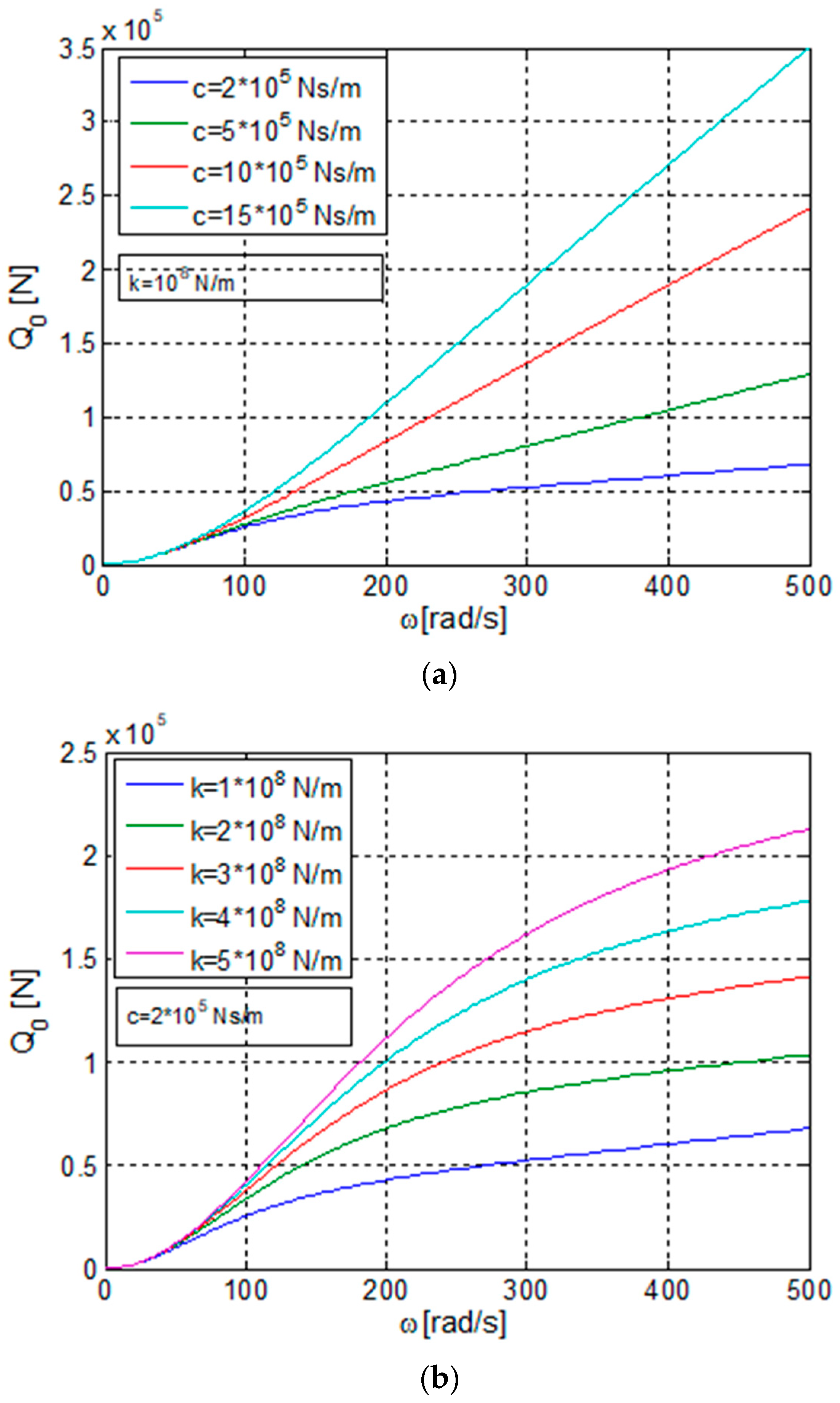
2.2. Transmitted Dynamic Force. Dynamic Force Transmitted in the Time Domain

The dynamic force Q transmitted by the Voigt–Kelvin viscous-elastic linear dynamic system may be complexly formulated as [24,25]:

$$\tilde{Q}=k\tilde{x}+c\dot{\tilde{x}}$$

(10)

where if it is taking into consideration $\tilde{x}={\tilde{X}}_0{e}^{j\omega t}$ and $\dot{\tilde{x}}=j\omega \tilde{x}$ results:

$$\tilde{Q}=\left(k+jc\omega \right)\tilde{x}$$

(11)

where inserting $\tilde{x}$ given by relation (3), $\tilde{Q}$ becomes:

$$\tilde{Q}=\frac{k+jc\omega }{{\left(k-m{\omega }^2\right)}^2+jc\omega }{F}_0{e}^{j\omega t}$$

(12)

For easier calculation operations, we insert the following notations:

$$\alpha =k, \beta =c\omega , \gamma =k-m{\omega }^2$$

In this case, relation (12) can be written down as:

$$\tilde{Q}=\frac{\alpha +j\beta }{{\gamma }^2+j\beta }{F}_0{e}^{j\omega t}$$

or

$$\tilde{Q}=\frac{\left(\alpha +j\beta \right)\left(\gamma -j\beta \right)}{{\gamma }^2+{\beta }^2}{F}_0{e}^{j\omega t}$$

from where, results:

$$\tilde{Q}=\left[\frac{\alpha \gamma +{\beta }^2}{{\gamma }^2+{\beta }^2}+j\frac{\beta \gamma -\alpha \beta }{{\gamma }^2+{\beta }^2}\right]F_0{e}^{j\omega t}$$

(13)

Using the notations q₁ and q₂ for the terms in (13), as follows

$${\mathit{q}}_{\mathbf{1}}=\frac{\mathbf{\alpha }\mathbf{\gamma }+{\mathbf{\beta }}^{\mathbf{2}}}{{\mathbf{\gamma }}^{\mathbf{2}}+{\mathbf{\beta }}^{\mathbf{2}}};{\mathit{q}}_{\mathbf{2}}=\frac{\mathbf{\beta }\mathbf{\gamma }-\mathbf{\alpha }\mathbf{\beta }}{{\mathbf{\gamma }}^{\mathbf{2}}+{\mathbf{\beta }}^{\mathbf{2}}}$$

and taking into account the fact that $\tilde{Q}={\tilde{Q}}_0{e}^{j\omega t}=Q_0{e}^{j\theta }{e}^{j\omega t}$ results:

$$Q_0\left(cos\theta +jsin\theta \right)=\left(q_1+j{q}_2\right)F_0$$

from where:

$$\{\begin{array}{c}{Q}_0^2=\left(q_1^2+q_2^2\right)F_0^2\\ tg\theta =\frac{q_1}{q_2}\end{array}$$

(14)

The sum $q_1^2+q_2^2$ results as

$${\mathit{q}}_{\mathbf{1}}^{\mathbf{2}}+{\mathit{q}}_{\mathbf{2}}^{\mathbf{2}}=\frac{{\left(\mathbf{\alpha }\mathbf{\gamma }+{\mathbf{\beta }}^{\mathbf{2}}\right)}^{\mathbf{2}}+{\left(\mathbf{\beta }\mathbf{\gamma }-\mathbf{\alpha }\mathbf{\beta }\right)}^{\mathbf{2}}}{{\left({\mathbf{\gamma }}^{\mathbf{2}}+{\mathbf{\beta }}^{\mathbf{2}}\right)}^{\mathbf{2}}}=\frac{{\mathbf{\alpha }}^{\mathbf{2}}+{\mathbf{\beta }}^{\mathbf{2}}}{{\mathbf{\gamma }}^{\mathbf{2}}+{\mathbf{\beta }}^{\mathbf{2}}},$$

which leads to the completion of the maximum dynamic force $Q_0$ as:

$$Q_0^2=\frac{{\alpha }^2+{\beta }^2}{{\gamma }^2+{\beta }^2}{F}_0^2$$

(15)

and of the phase $\theta$ from the transmitted dynamic force $Q\left(t\right)$ and the harmonic perturbing force $F\left(t\right)$, as follows:

$$tan\theta =\frac{\beta \gamma -\alpha \beta }{\alpha \gamma +{\beta }^2}$$

(16)

Replacing notations $\alpha ,\beta$ and $\gamma$ with the previously established physical measures, the expressions of the dynamic parameters of the transmitted forces become:

$$Q_0\left(\omega \right)=Q_0=F_0\sqrt{\frac{k^2+c^2{\omega }^2}{{\left(k-m{\omega }^2\right)}^2+c^2{\omega }^2}}$$

(17)

where:

$Q_0$ is the amplitude of the instantaneous dynamic force transmitted (the maximum dynamic force)

$$tan\theta =\frac{-mc{\omega }^3}{k{\left(k-m{\omega }^2\right)}^2+c^2{\omega }^2}$$

(18)

$\mathit{\theta }$ is the phase between the transmitted dynamic force $Q\left(t\right)$ and the perturbing force $F\left(t\right)$[26,27].

In this case, the expression of the transmitted dynamic force is:

$$Q\left(t\right)=Q_{0}sin\left(\omega t+\theta \right)$$

(19)

For the discrete viscous amortization, taking into account the relative measures $\mathsf{\Omega }$ and $\zeta$ results:

$$Q_0\left(\zeta , \mathsf{\Omega }\right)=F_0\sqrt{\frac{1+{\left(2\zeta \mathsf{\Omega }\right)}^2}{{\left(1-{\mathsf{\Omega }}^2\right)}^2+{\left(2\zeta \mathsf{\Omega }\right)}^2}}$$

(20)

$$tan\theta =-\frac{2\zeta {\mathsf{\Omega }}^3}{{\left(1-{\mathsf{\Omega }}^2\right)}^2+{\left(2\zeta \mathsf{\Omega }\right)}^2}$$

(21)

The amplitude of the transmitted force $Q_0$ is represented in Figure 3.

Figure 3a shows that, for a constant value of stiffness k, in postresonance regime mode ($\omega \ge 300\mathrm{rad}/\mathrm{s}$) the maximum transmitted force Q₀ increases linearly with increasing pulsation ω of the disturbing force $F\left(t\right)=F_{0}sin\left(\omega t\right)$.

In Figure 3b, for the constant damping value c, in postresonance regime mode, the maximum transmitted force Q₀ increases asymptotically to a limit value by a slow variation in relation to the increase of the pulsation ω of the disturbing force F.

Transmitted force $Q=Q\left(t\right)$ may be expressed in relation with the displacement $x=x\left(t\right)$, taking into account that $x=Asin\left(\omega t+\phi \right)$ and $\dot{x}=\omega Acos\left(\omega t+\phi \right)$.

If it replaces $cos\left(\omega t+\phi \right)=\pm \sqrt{1-\frac{x^2}{A^2}}$ in the expression of the speed $\dot{\mathit{x}}$, [28,29,30], the expression of velocity becomes:

$$\dot{x}=\pm \omega A\sqrt{1-\frac{x^2}{A^2}},\mathrm{where}A=A\left(\omega \right).$$

In this case, the transmitted force function of $x$ and $\dot{x}$ as $Q\left(x, \dot{x}\right)=kx+c\dot{x}$ may be written down only in relation with $x$, as follows:

$$Q\left(\omega ,x\right)=kx\pm c\omega \sqrt{A^2\left(\omega \right)-x^2}$$

(22)

where $A\left(\omega \right)=A$ is the amplitude given by the relation (4).

Using the relative quantities $\mathsf{\Omega }=\frac{\omega }{{\omega }_n}$ and $\zeta =\frac{c}{2m{\omega }_n}$, relation (22) may be written:

$$Q\left(\mathsf{\Omega },x\right)=k\left[x\pm \left(2\zeta \mathsf{\Omega }\right)\sqrt{A^2\left(\zeta ,\mathsf{\Omega }\right)-x^2}\right]$$

(23)

where $A\left(\zeta ,\mathsf{\Omega }\right)$ is the amplitude given by the relation (8).

Figure 4 presents the hysteresis loops parameterized by the discrete variation of the excitation pulsation ω. The family of hysteresis loops in steady-state mode, for 5 values ω of the pulsation of the disturbing force F, highlights the extent to which the effect of energy dissipation in the dynamic system can be evaluated, provided that the following parameters are kept constant: mass m, stiffness k, damping c and the first moment of the rotating eccentric masses $m_{0}r$.

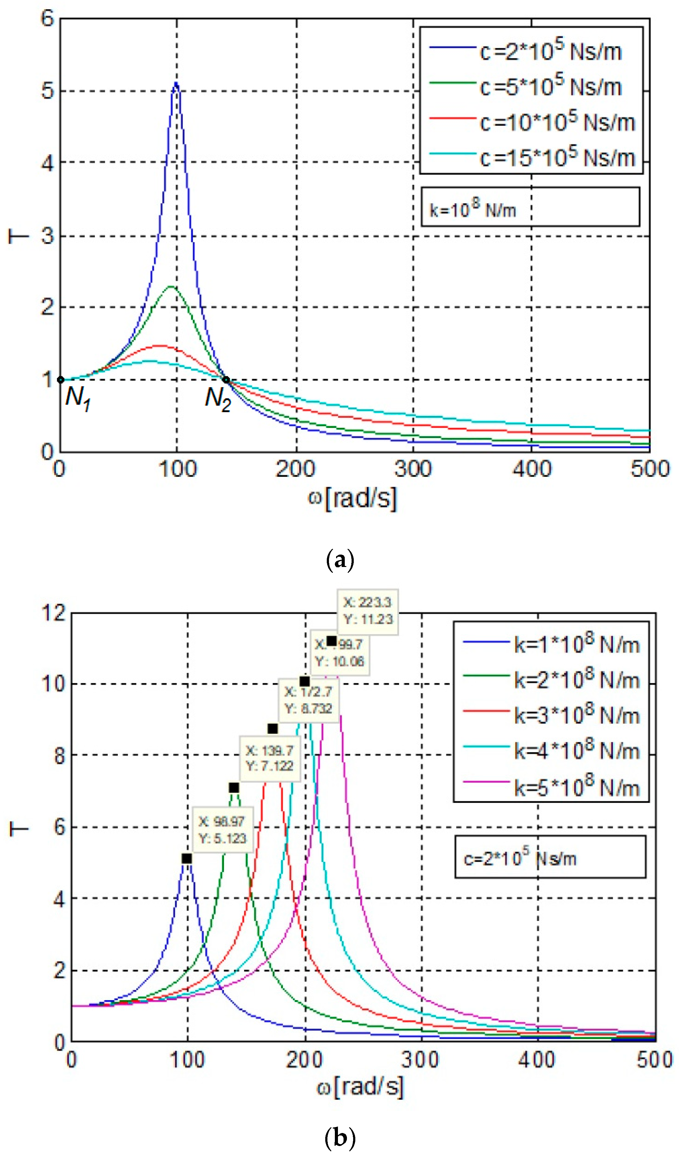
2.3. Dynamic Insulation Capacity

The T coefficient of transmissibility of the force $Q\left(t\right)=Q_{0}sin\left(\omega t+\phi \right)$, in relation to the harmonic perturbing force F(t) = F₀sinωt, is defined as the relation between the amplitude of the transmitted force $Q_0$ and the amplitude of the perturbative force F₀, as [10,12,31]:

$$T=\frac{Q_0}{F_0}$$

(24)

or

$$T=\left|\frac{Q_0}{F_0}\right|$$

(25)

The degree of dynamic insulation I is defined as follows:

$$I=\left(1-T\right)$$

(26)

or punctually

$$I=\left(1-T\right)100, [\%]$$

(27)

Taking account of the expressions (17) and (20), the transmissibility coefficient T may be expressed as follows:

$$T\left(\omega \right)=\left|\frac{Q_0\left(\omega \right)}{F_0\left(\omega \right)}\right|=\sqrt{\frac{k^2+c^2{\omega }^2}{{\left(k-m{\omega }^2\right)}^2+c^2{\omega }^2}}$$

(28)

$$T\left(\zeta , \mathsf{\Omega }\right)=\left|\frac{Q_0\left(\zeta , \mathsf{\Omega }\right)}{F_0\left(\mathsf{\Omega }\right)}\right|=\sqrt{\frac{k^2+{\left(2\zeta \mathsf{\Omega }\right)}^2}{{\left(1-{\mathsf{\Omega }}^2\right)}^2+{\left(2\zeta \mathsf{\Omega }\right)}^2}}$$

(29)

The transmissibility coefficient function of $\omega$ and c is expressed by the variation $T\left(\omega \right)$, as presented in Figure 5. It is found that the neutral point N₁ has coordinates ${\omega }_{N_1}$ and $T_{N_1}$ independent from the discrete variation of c. In relation (28) it is necessary to comply with the condition $k^2={\left(k-m{\omega }^2\right)}^2$, from where it results ${\omega }^2=2\frac{k}{m}$ or $\omega =\sqrt{2}{\omega }_n={\omega }_{N_1}$. Replacing in the expression of $T\left(\omega \right)$ it results $T_{N_1}\left(\omega \right)=1$.

The maximum value of $T\left(\omega \right)$ corresponds to point $M_1({\omega }_{M_1},T_{M_1}^{max})$, with the condition $\frac{dT\left(\omega \right)}{d\omega }=0$. The following quantities result:

$${\omega }_{M_1}=\frac{2k}{c}\sqrt{\sqrt{1+\frac{2c^2}{km}}-\frac{2k}{c}}$$

(30)

$$T_{M_1}^{max}\left(\omega \right)=\frac{1}{\sqrt{2}}\delta \frac{1}{\sqrt{\sqrt{1+2\delta }+\delta \left(\delta -1\right)-1}}$$

(31)

where $\delta =\frac{c^2}{km}$ or $\delta =\frac{4{\zeta }^{2}km}{km}=4{\zeta }^2$.

The graphs of the transmissibility T function of $\mathsf{\Omega }$ and $\zeta$ are presented in Figure 6. In this case, the coordinates of the neutral point N₂ result from relation (29), with the condition $1={\left(1-{\mathsf{\Omega }}^2\right)}^2$, from where ${\mathsf{\Omega }}_{N_2}=\sqrt{2}$ and $T_{N_2}\left(\zeta , \mathsf{\Omega }\right)=1$.

The point of maximum M₂ of function $T\left(\zeta , \mathsf{\Omega }\right)$ has coordinates ${\omega }_{M_2}$ and $T_{M_2}\left(\zeta , \mathsf{\Omega }\right)$, which emerge from the condition $\frac{d{T}_{M_2}}{d\mathsf{\Omega }}=0$. Thus, the following results:

$${\mathsf{\Omega }}_{M_2}=\frac{1}{2\zeta }\frac{1}{\sqrt{\sqrt{1+8{\zeta }^2}-1}}$$

(32)

$$T_{M_1}^{max}\left(\zeta , \mathsf{\Omega }\right)=\frac{4}{\sqrt{2}}{\zeta }^2\frac{1}{\sqrt{\sqrt{1+8{\zeta }^2}+4{\zeta }^2\left(2{\zeta }^2-1\right)-1}}$$

(33)

Figure 5a shows the transmissibility T of the vibration, at constant stiffness k and four discrete values of damping c, as a function of the pulsation ω of the disturbing force F.

Figure 5b shows the transmissibility T of the vibration, at constant damping c and five values of stiffness k, as a function of the pulsation ω of the disturbing force F. The variation graphs of the transmissibility T for the 5 values of stiffness k show the rightward displacement of the resonance point (towards higher values of the pulsation ω) with increasing stiffness k at constant damping c. The maximum values of the transmissibility T are on the straight line described by the equation $T\left(\omega \right)=0.26166+0.04912\omega$ (for $\omega >100 \mathrm{rad}/\mathrm{s}$). These points of maximum amplitude characterize the phenomenon of transmissibility resonance of the system.

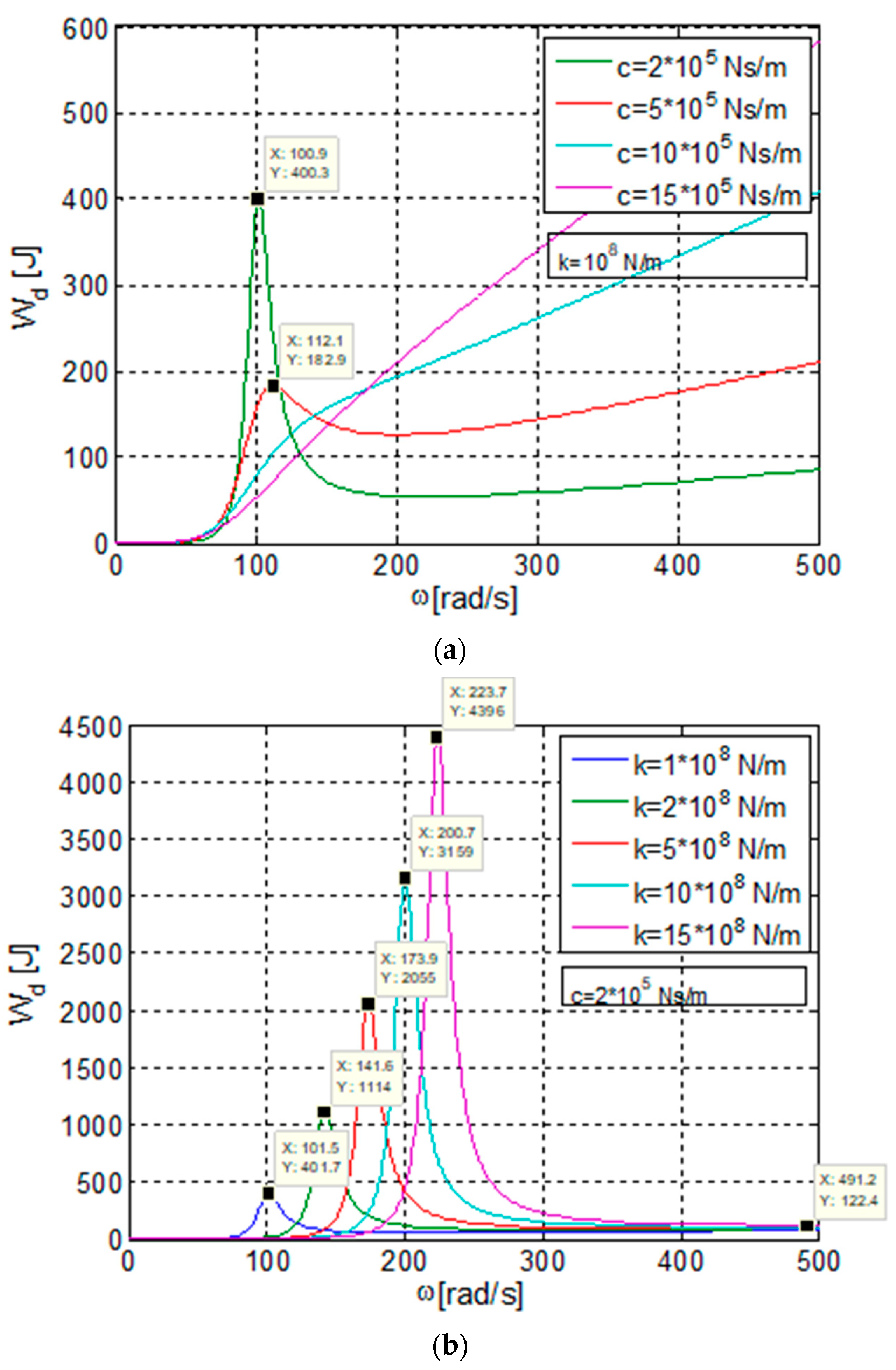
2.4. Dissipated Energy

The dissipated energy on the viscous element is directly proportional with the coefficient of the linear viscous amortization c with pulsation $\omega$ of the excitation movement and the square of the amplitude of instantaneous displacement A [1,5,32,33].

In this case, the expression of the dissipated energy may be written as:

$$W_d=\pi c\omega A^2$$

(34)

For the disruptive force $F\left(t\right)=m_0\mathrm{r}{\omega }^2\mathit{sin}\omega t$, the following expressions for the dissipated energy are obtained, as follows:

$$W_d\left(c,\omega \right)=\pi c{\left(m_{0}r\right)}^2\frac{{\omega }^5}{{\left(k-m{\omega }^2\right)}^2+c^2{\omega }^2}$$

(35)

$$W_d\left(\zeta , \mathsf{\Omega }\right)=\pi k{\left(\frac{m_{0}r}{m}\right)}^2\frac{2\zeta {\mathsf{\Omega }}^5}{{\left(1-{\mathsf{\Omega }}^2\right)}^2+{\left(2\zeta \mathsf{\Omega }\right)}^2}$$

(36)

Figure 6a,b present the variation of the dissipated energy ${\mathit{W}}_{\mathit{d}}$ function of the pulsation ω, damping c and stiffness k, according to relation (35).

Figure 6a shows the graphs of the dissipated energy for the discrete variation of damping c and constant stiffness k, function of the pulsation ω of the harmonic disturbing force F. The analysis of the graphs shows that, for damping values $c\ge {10}^6 \mathrm{Ns}/\mathrm{m}$, the dissipated energy increases significantly with the pulsation ω of the disturbing force F.

The graphs from Figure 6b show that, for constant damping c, at the discrete variation of the stiffness k, the maximum values of the dissipated energy (at the resonance) strongly increase with the pulsation ω of the disturbing force F.

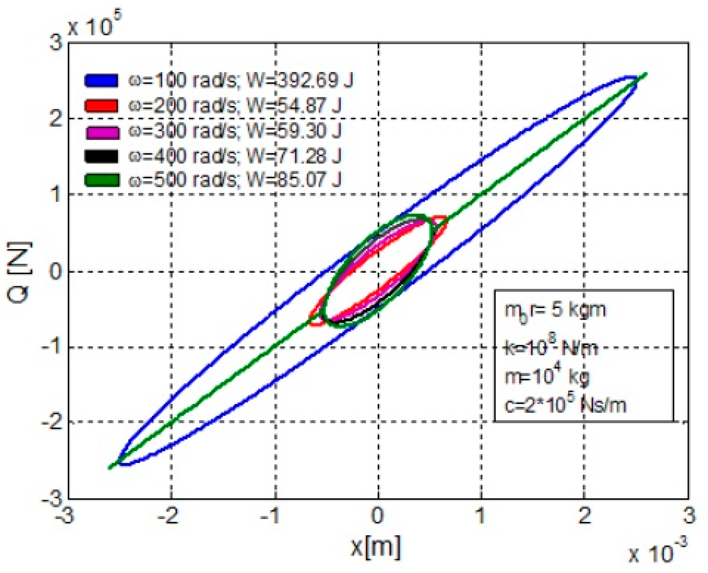
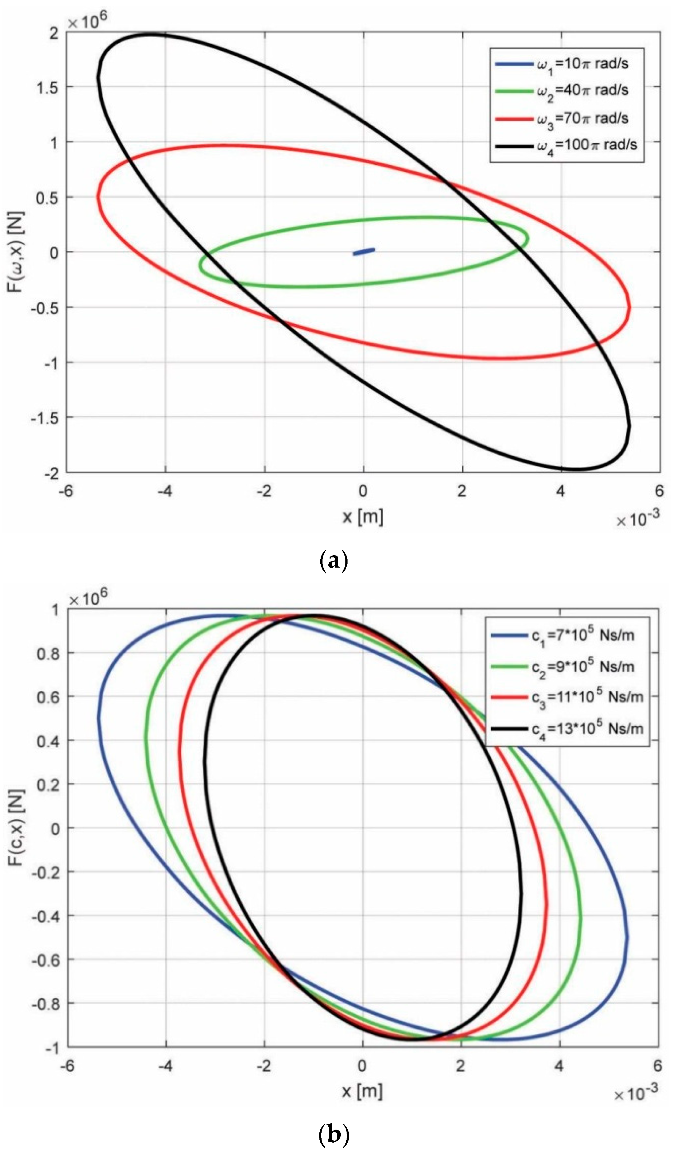
2.5. Representation of the Hysteresis Loop

The equation of the hysteresis loop, that is of the ellipsis as function of connection between the excitation force $F=F\left(t\right)=F_0\mathit{sin}\omega t$ and instantaneous displacement $x=x\left(t\right)=A\mathit{sin}\left(\omega t+\phi \right)$, may be deduced by eliminating the temporal parameter between the two expressions $F\left(t\right)$ and $x\left(t\right)$[10,28].

In this case, it may be written down as trigonometrically developed form the expression of $x\left(t\right)$ as follows:

$$x=A\mathit{sin}\omega t\mathit{cos}\phi +A\mathit{sin}\phi \mathit{cos}\omega t$$

(37)

where

$$\mathit{sin}\omega t=\frac{F}{F_0};\mathit{cos}\omega t=\pm \sqrt{1-\frac{F^2}{F_0^2}}$$

so that relation (37) becomes:

$$\frac{x}{A}=\frac{F}{F_0}\mathit{cos}\phi \pm \mathit{sin}\phi \sqrt{1-\frac{F^2}{F_0}}$$

(38)

If it inserts notations $X=\frac{x}{A}$ and $\mathsf{\Phi }=\frac{F}{F_0}$ as follows:

$$X=\mathsf{\Phi }\mathit{cos}\phi \pm \mathit{sin}\phi \sqrt{1-{\mathsf{\Phi }}^2}$$

(39)

$${\mathsf{\Phi }}^2+X^2-2\mathsf{\Phi }X\mathit{cos}\phi ={\mathit{sin}}^2\phi$$

with solution

$${\mathsf{\Phi }}_{1,2}=X\mathit{cos}\phi \pm \mathit{sin}\phi \sqrt{1-\frac{{\mathrm{x}}^2}{{\mathrm{A}}^2}}$$

it results

$$F=F_0\left[\frac{x}{A}\mathit{cos}\phi \pm \mathit{sin}\phi \sqrt{1-\frac{{\mathrm{x}}^2}{{\mathrm{A}}^2}}\right]$$

(40)

with real solutions for $-A\le x\le +A$.

If the amplitude of the harmonic perturbing force is $F_0=m_0\mathrm{r}{\omega }^2$, then results:

$$F\left(x\right)=m_0\mathrm{r}{\omega }^2\left[\frac{x}{A}\mathit{cos}\phi \pm \mathit{sin}\phi \sqrt{1-\frac{{\mathrm{x}}^2}{{\mathrm{A}}^2}}\right]$$

(41)

Functions $sin\phi$ and $cos\phi$ result from relation (7) as follows:

$$\mathit{sin}\phi =-\frac{c\omega }{\sqrt{{\left(k-m{\omega }^2\right)}^2+c^2{\omega }^2}}$$

(42)

$$\mathit{cos}\phi =\frac{k-m{\omega }^2}{\sqrt{{\left(k-m{\omega }^2\right)}^2+c^2{\omega }^2}}$$

(43)

Figure 7a,b present the hysteresis loops for the discrete variation of ω and for the discrete variation of c.

The hysteresis loops shown in Figure 7a,b highlight the following aspects of the dynamic behavior of the system:

• hysteresis ellipses are in quadrants II and IV due to the inertial effect of the mass m of the working part of the technological equipment;
• for constant values of stiffness k and damping c, the areas of the hysteresis ellipses at four discrete values of the pulsation ω of the harmonic disturbing force F change significantly; thus, at values of $\mathbf{\omega }\ge \mathbf{70}\mathbf{\pi } rad/s$ the area of the hysteresis ellipses and, implicitly, the dissipated energy W increase significantly;
• for constant values of the stiffness k and the pulsation ω of the disturbing force F, at the discrete variation of the damping c, distinct values of the areas of the hysteresis ellipses and, implicitly, of the dissipated energies W, are obtained; as the damping coefficient c increases, the hysteresis ellipse rotates clockwise.

This case study was performed on a vibrating machine model with the static moment of the dynamic unbalance masses $m_{0}r=5 \mathrm{kgm}$; mobile mass $m={10}^4 \mathrm{kg}$; viscoelastic material in technological processing (clay soil) with discrete variable stiffness from ${10}^5\mathrm{kN}/\mathrm{m}$ up to $5\times {10}^5\mathrm{kN}/\mathrm{m}$ and viscous damping coefficient c from $2\times {10}^2 \mathrm{kNs}/\mathrm{m}$ up to $15\times {10}^2\mathrm{kNs}/\mathrm{m}$, the excitation force pulsation ω in steady-state regime with values from 200 rad/s up to 500 rad/s [16,34,35].

3. Conclusions

Based on the schematized dynamic model and the hypothesis of linear behavior in steady-state dynamic regime in postresonance, the technological vibrating machines can be evaluated based on the calculation relationships established in this article.

Thus, the following conclusions can be summarized:

• the amplitude of the technological vibrations during the postresonance regime is relatively constant, its variation being insignificant for the working process for values of the excitation pulsation ω higher than 2–4 times in relation to the resonance pulsation;
• the modification to the technological values necessary for the work process can be done during the postresonance regime, $\mathbf{\omega }=\left(\mathbf{2}\dots \mathbf{4}\right)\sqrt{\frac{\mathit{k}}{\mathit{m}}}$, using relation ${\mathit{m}}_{\mathit{0}}\mathit{r}=\mathit{A}\mathit{m}$ from where result the amplitudes ${\mathit{A}}_{\mathbf{1}}$, ${\mathit{A}}_{\mathbf{2}}$, … ${\mathit{A}}_{\mathit{n}}$ for various values of the static moment ${\left({\mathit{m}}_{\mathbf{0}}\mathit{r}\right)}_{\mathbf{1}}$, ${\left({\mathit{m}}_{\mathbf{0}}\mathit{r}\right)}_{\mathbf{2}}$, …, ${\left({\mathit{m}}_{\mathbf{0}}\mathit{r}\right)}_{\mathit{n}}$ at the same value of mobile mass m;
• the force transmitted to the processed material and the energy dissipated by the system at processing for the postresonance regime are given by the calculation relations established and verified in practical cases;
• the hysteresis loops illustrate both the variation of the force in relation to the instantaneous displacement x(t) and the dissipated energy depending on the area of the elliptical surface.

It results that the parametric analysis for any dynamic regime in the technological process can be conducted based on the calculation relationships and the graphical representations that must individualize the dynamic model by its structural parameters (m, k, c) and excitation characteristics ($m_{0}r$, ω).

Potential multidisciplinary applications of the paper:

-

industry: smart building and road vibrating equipment with real-time management of the technological parameters using analogue sensors, digital data processing and Neural Networks and Neuro-Fuzzy techniques [16,36];

-

environment protection: reduction of harmful vibrations transmitted by dynamic action equipment through foundations (passive/active damping in real-time);

-

health research: dynamic analysis of the human body modeled as a biomechanical system with (m,c,k) linear characteristics.

The limitations of the analyzed model may appear due to the following causes:

-

the hypothesis of linearity of damping and elasticities;

-

mass/moment of inertia modifications during technological processes;

-

a more complex rheological model of the interaction between the vibrating machine and the working environment that can radically change the dynamic response of the system and its operating energy parameters.

References

1. Rao, M. Mechanical Vibrations; Addison-Wesley Pub. Co.: Boston, MA, USA, 1986. [Google Scholar]
2. Sireteanu, T.; Giuclea, M.; Mitu, A.M. An analitical approach for approximation of experimental hysteretic by Bouc.-Wen model. Procc. Rom. Acad. Ser. A 2009, 10, 43–54. [Google Scholar]
3. Nițu, M.C. Parametric evaluation of the vibrating screens for performance assurance in sorting mineral aggregates. ACTA Teh. Napoc. Appl. Math. Mech. Eng. 2020, 63, 331–334. [Google Scholar]
4. Stamatiade, C. The influences upon the quality of the mineral aggregates induced by technological vibrations during the sorting process. Rom. J. Acoust. Vib. 2009, VI, 1. [Google Scholar]
5. Bratu, P.; Dobrescu, C. Evaluation of the Dissipated Energy in Vicinity of the Resonance, depending on the Nature of Dynamic Excitation. Rom. J. Acoust. Vib. 2019, 16, 66–71. [Google Scholar]
6. Vasile, O. Active vibration control for viscoelastic amortization systems under the action of inertial forces. Rom. J. Acoust. Vib. 2017, 14, 54–58. [Google Scholar]
7. Bratu, P. Multibody system with elastic connections for dynamic modeling of compactor vibratory rollers. Symmetry 2020, 12, 1617. [Google Scholar] [CrossRef]
8. Dragan, N. Nonlinear approach of the systems between the dynamic modeling difficulties and the advantages of using it in mechanical designing. Rom. J. Acoust. Vib. 2010, 2, 2. [Google Scholar]
9. Dobrescu, C.F. Analysis of Dynamic Earth Stiffness depending on Structural Parameters in the Process of Vibration Compaction. Rom. J. Acoust. Vib. 2019, 16, 174–177. [Google Scholar]
10. Dobrescu, C.F. Dynamic Response of the Newton Voigt–Kelvin Modelled Linear Viscoelastic Systems at Harmonic Actions. Symmetry 2020, 12, 1571. [Google Scholar] [CrossRef]
11. Pințoi, R.; Bordos, R.; Braguța, E. Vibration Effects in the Process of Dynamic Compaction of Fresh Concrete and Stabilized Earth. J. Vib. Eng. Technol. 2017, 5, 247–254. [Google Scholar]
12. Bejan, S. Dynamic Response Analysis of the Road System Compaction According to the Forced Vibration Mode. Rom. J. Acoust. Vib. 2014, XI, 164–166. [Google Scholar]
13. Capatana, G.F. Dynamic simulation of the vibratory roller-terrain interaction using an elastoplastic approach. In Annals of University Dunărea de Jos din Galaţi, XIV, Mechanical Engineering; Galati University Press: Galati, Romania, 2013. [Google Scholar]
14. Le Tallec, P. Introduction à la Dynamique des Structures; Cépaduès: Toulouse, France, 2000. [Google Scholar]
15. Radeș, M. Mechanical Vibrations; Editura Printech: București, Romania, 2006. [Google Scholar]
16. Edincliler, A.; Cabalar, A.F.; Cevik, A. Modelling dynamic behaviour of sand–waste tires mixtures using Neural Networks and Neuro-Fuzzy. Eur. J. Environ. Civ. Eng. 2013, 17, 720–741. [Google Scholar] [CrossRef]
17. Inman, D. Vibration with Control; John Wiley & Sons Ltd.: London, UK, 2007. [Google Scholar]
18. Adam, D.; Kopf, F. Theoretical Analysis of Dynamically Loaded Soils, European Workshop: Compaction of Soils and Granular Materials; ETC11 of ISSMGE: Paris, France, 2000. [Google Scholar]
19. Mooney, M.A.; Rinehart, R.V. In-Situ Soil Response to Vibratory Loading and Its Relationship to Roller-Measured Soil Stiffness. J. Geotech. Geoenviron. Eng. ASCE 2009, 135, 1022–1031. [Google Scholar] [CrossRef] [Green Version]
20. Mooney, M.A.; Rinehart, R.V.; White, D.J.; Vennapusa, P.K.; Facas, N.W.; Musimbi, O.M. Intelligent Soil Compaction Systems; NCHRP project 21-09 final report; Transportation Research Board: Washington, DC, USA, 2010. [Google Scholar]
21. Adam, D. Continuous Compaction Control (CCC) with Vibratory Roller, GeoEnvironment Revue; Balkema Rotterdam: Bouazza, Morocco, 1997. [Google Scholar]
22. Adam, D.; Kopf, F. Sophisticated Roller Compaction Technologies and Roller-Integrated Compaction Control, Compaction of Soils-Granulates and Powders; Editura Kolymbas & Fellin: Rotterdam, The Netherlands, 2000. [Google Scholar]
23. Forssblad, L. Vibratory Soil and Rock Fill Compaction; Robert Olsson Tryckeri AB: Stockholm, Sweden, 1981. [Google Scholar]
24. Floss, R.; Kloubert, H.-J. Newest Developments in Compaction Technology. In Proceedings of the European Workshop Compaction of Soils and Granular Materials, Presses Ponts et Chaussées, Paris, France, 19 May 2000; pp. 247–261. [Google Scholar]
25. Capatana, G.F. Dynamic behaviour of complex interaction between vibratory drum equipment and natural terrain based on rheological evaluations. In Proceedings of the 10th HSTAM International Congress on Mechanics Chania, Crete, Greece, 25–27 May 2013. [Google Scholar]
26. Adam, D.; Kopf, F. Operational Devices for Compaction Optimization and Quality Control (Continuous Compaction Control & Light Falling Weight Device). In Proceedings of the International Seminar on Geotechnics in Pavement and Railway Design and Construction, Athens, Greece, 16–17 December 2004; pp. 97–106. [Google Scholar]
27. Anderegg, R. ACE Ammann Compaction Expert–Automatic Control of the Compaction. In Proceedings of the European Workshop Compaction of Soils and Granular Materials, Paris, France, 19 May 2000; pp. 229–236. [Google Scholar]
28. Bratu, P. Hysteretic Loops in Correlation with the Maximum Dissipated Energy, for Linear Dynamic Systems. Symmetry 2019, 11, 315. [Google Scholar] [CrossRef] [Green Version]
29. Brandl, H.; Adam, D. Sophisticated continuous compaction control of soils and granular materials. In Proceedings of the 14th International Conference on Soil Mechanics & Foundation Engineering, Hamburg, Germany, 6–12 September 1997; Volume 1, pp. 31–36. [Google Scholar]
30. Mooney, M.A.; Rinehart, R.V. Field Monitoring of Roller Vibration During Compaction of Subgrade Soil. J. Geotech. Geoenviron. Eng. ASCE 2007, 133, 257–265. [Google Scholar] [CrossRef]
31. Tonciu, O. Parametric analysis of vibrating equipment for the insertion of piles into the ground. ACTA Tech. Napoc. Appl. Math. Mech. Eng. 2020, 63, 95–100. [Google Scholar]
32. Bejan, S. Rheological Models of the Materials for the Road System in the Compaction Process. Rom. J. Acoust. Vib. 2014, XI, 67. [Google Scholar]
33. Capatana, G.F. Analysis of the Dynamics of Vibratory Compactor Rollers for Road Works. Doctoral Thesis, “Dunarea de Jos” University of Galati, Galați, Romania, 2014. [Google Scholar]
34. Pinţoi, R. Dependence of the Concrete Strength on the Duration of the Compaction by Vibration Process. Rom. J. Acoust. Vib. 2015, 11, 67. [Google Scholar]
35. Spanu (Stefan), G.C.; Capatana, G.F.; Potirniche, A. Analysis of the Transmissibility Ratio and the Isolation Degree of the Vibration for 1DOF Mechanical Systems with Zener Viscous Damping Model. Synth. Theor. Appl. Mech. 2019, 10, 43–46. [Google Scholar]
36. Thakur, N.; Han, C.Y. An Ambient Intelligence-Based Human Behavior Monitoring Framework for Ubiquitous Environments. Information 2021, 12, 81. [Google Scholar] [CrossRef]
Figure 1. Scheme of the linear dynamic system (MCK) excited with force F ( t ) = m 0 r ω 2 s i n ( ω t ) , where F 0 = F 0 ( ω ) = m 0 r ω 2 (a) Voigt–Kelvin model dynamic system; (b) eccentric body of the dynamic imbalance with mass 1 2 m 0 and eccentricity r , in relation to the axis of rotation, with normal passing through O.
Symmetry 14 00539 g001
Figure 2. (a) The amplitude of steady-state vibration in dynamic regime—variation of amplitude function of ω and c; (b) The amplitude of steady-state vibration in dynamic regime—variation of amplitude function of ω and k.
Symmetry 14 00539 g002
Figure 3. The amplitude of the transmitted force (maximum transmitted force). (a) The amplitude of the transmitted force Q 0 function of ω and c; (b) The amplitude of the transmitted force Q 0 function of ω and k.
Symmetry 14 00539 g003
Figure 4. Hysteresis loops Q-x for the discrete variation of ω.
Symmetry 14 00539 g004
Figure 5. Transmissibility T=|T| (a) variation of T function of ω and c; (b) variation of T function of ω and k.
Symmetry 14 00539 g005
Figure 6. (a) Dissipated energy function of ω and c (at constant stiffness k); (b) dissipated energy function of ω and k (at constant damping c).
Symmetry 14 00539 g006
Figure 7. (a) Hysteresis loops F-x for F 0 = m 0 r ω 2 —discrete variation of ω ( m 0 r = 5   kgm , m = 10,000   kg ). (b) Hysteresis loops F-x for F 0 = m 0 r ω 2 —discrete variation of c ( m 0 r = 5   kgm , m = 10,000   kg ).
Symmetry 14 00539 g007
Publisher’s Note: MDPI stays neutral with regard to jurisdictional claims in published maps and institutional affiliations.