An Efficient Algorithm for Solving the Matrix Optimization Problem in the Unsupervised Feature Selection

Abstract

In this paper, we consider the symmetric matrix optimization problem arising in the process of unsupervised feature selection. By relaxing the orthogonal constraint, this problem is transformed into a constrained symmetric nonnegative matrix optimization problem, and an efficient algorithm is designed to solve it. The convergence theorem of the new algorithm is derived. Finally, some numerical examples show that the new method is feasible. Notably, some simulation experiments in unsupervised feature selection illustrate that our algorithm is more effective than the existing algorithms.

1. Introduction

Throughout this paper, we use $R^{n\times m}$ to denote the set of $m\times n$ real matrices. We write $B\ge 0$ if the matrix B is nonnegative. The symbols $Tr(B),B^T$ stand for the trace and transpose of the matrix B, respectively. The symbol $\parallel \alpha \parallel$ stands for the $l_2$-norm of the vector $\alpha$, i.e., $\parallel \alpha \parallel ={({\alpha }^T\alpha )}^{\frac{1}{2}}$. The symbol ${\parallel B\parallel }_F$ stands for the Frobenius norm of the matrix B. The symbol $I_p$ stands for the $p\times p$ identity matrix. For the matrices A and B, $A\odot B$ denotes the Hadamard product of A and B. The symbol $max\{x,y\}$ represents the greater of x and y.

In this paper, we consider the following symmetric matrix optimization problem in unsupervised feature selection.

Problem 1.

Given a matrix $A\in R^{n\times m}$, consider the symmetric matrix optimization problem

$$\underset{X,Y}{min}\frac{1}{2}{\parallel A-AXY\parallel }_F^2,s.t.X\ge 0,Y\ge 0,X^{T}X=I_p.$$

(1)

Here $A=[f_1,f_2,\cdots ,f_m]\in R^{n\times m}$ is the data matrix, $X\in R^{m\times p}$ is the indicator matrix (feature weight matrix) and $Y\in R^{p\times m}$ is the coefficient matrix.

Problem 1 arises in unsupervised feature selection, which is an important part of machine learning. This can be stated as follows. Data from image processing, pattern recognition and machine learning are usually high-dimensional data. If we deal with these data directly, this may increase the computational complexity and the memory of the algorithm. In particular, it may lead to the overfitting phenomenon for the machine learning model. Feature selection is a common dimension reduction method, the goal of which is to find the most representative feature subset from the original features, that is to say, for a given original high-dimensional data matrix A, we must find out the relationship between the original feature space and the subspace generated by the selected feature. Feature selection can be formalized as follows.

$$\underset{I}{min}d(Span(A),Span(A_c))=\Vert A_{I^c}-A_I{Y\Vert }_F,s.t.\left|I\right|=k,$$

(2)

where I denotes the index set of the selected features and Y is the coefficient matrix of the initial feature space in the selected features. From the viewpoint of matrix factorization, feature selection is expressed as follows

$$\underset{X,Y}{min}\frac{1}{2}\Vert A-AXY\Vert ,s.t.X\ge 0,X^{T}X=I_p.$$

(3)

Considering that the data in practical problems are often nonnegative, we add a constraint to guarantee that any feature is described as the positive linear combination of the selected features, so the problem in (3) can be rewritten as in (1).

In the last few years, many numerical methods have been proposed for solving optimization problems with nonnegative constraints, and these methods can be broadly classified into two categories: alternating gradient descent methods and alternating nonnegative least squares methods. The most commonly used alternating gradient descent method is the multiplicative update algorithm [1,2]. Although the multiplicative update algorithm is simple to implement, it lacks a convergence guarantee. The alternating nonnegative least squares method is used to solve nonnegative subproblems. Many numerical methods, such as the active method [3], the projected gradient method [4,5], the projected Barzilai–Borwein method [6,7], the projected Newton method [8] and the projected quasi-Newton method [9,10], have been designed to solve these subproblems.

For optimization problems with orthogonal constraints, which are also known as optimization problems on manifolds, there are many algorithms to solve this type of problem. In general, these can be divided into two categories: the feasible method and the infeasible method. The feasible method means that the variance obtained after each iteration must satisfy the orthogonal constraint. Many traditional optimization algorithms, such as the gradient method [11], the conjugate method [12], the trust-region method [13], Newton method [8] and the quasi-Newton method [14], can be used to deal with optimization problems on manifolds. Wen and Yin [15] proposed the CMBSS algorithm, which combined the Cayley transform and the curvilinear search approach with BB steps. However, the computational complexity increases when the number of variables or the amount of data increases, resulting in the low efficiency of this algorithm. Infeasible methods can overcome this disadvantage when facing high-dimensional data. In 2013, Lai and Osher [16] proposed a splitting method based on Bregman iteration and the ADMM method for orthogonality constraint problems. The SOC method is a valid and efficient method for solving the convex optimization problems but the proof of its convergence is still uncertain. Thus, Chen et al. [17] put forward a proximal alternating augmented Lagrangian method to solve such optimization problems with a non-smooth objective function and non-convex constraint.

Some unsupervised feature selection algorithms based on matrix decomposition have been proposed and have achieved good performance, such as SOCFS, MFFS, RUFSM, OPMF and so on. Based on the orthogonal basis clustering algorithm, SOCFS [18] does not explicitly use the pre-computed local structure information for data points represented as additional terms of their objective functions, but directly computes latent cluster information by means of the target matrix, conducting orthogonal basis clustering in a single unified term of the objective function. In 2017, Du S et al. [19] proposed RUFSM, in which robust discriminative feature selection and robust clustering are performed simultaneously under the $l_{2,1}$-norm, while the local manifold structures of the data are preserved. MFFS was developed from the viewpoint of subspace learning. That is, it treats feature selection as a matrix factorization problem and introduces an orthogonal constraint into its objective function to select the most informative features from high-dimensional data.

OPMF [20] incorporates matrix factorization, ordinal locality structure preservation and inner-product regularization into a unified framework, which can not only preserve the ordinal locality structure of the original data, but also achieve sparsity and low redundancy among features.

However, research into Problem 1 is very scarce as far as we know. The greatest difficulty is how to deal with the nonnegative and orthogonal constraints, because the problem has highly structured constraints. In this paper, we first use the penalty technique to deal with the orthogonal constraint and reformulate Problem 1 as a minimization problem with nonnegative constraints. Then, we design a new method for solving this problem. Based on the auxiliary function, the convergence theorem of the new method is derived. Finally, some numerical examples show that the new method is feasible. In particular, some simulation experiments in unsupervised feature selection illustrate that our algorithm is more efficient than the existing algorithms.

The rest of this paper is organized as follows. A new algorithm is proposed to solve Problem 1 in Section 2 and the convergence analysis is given in Section 3. In Section 4, some numerical examples are reported. Numerical tests on the proposed algorithm applied to unsupervised feature selection are also reported in that section.

2. A New Algorithm for Solving Problem 1

In this section we first design a new algorithm for solving Problem 1; then, we present the properties of this algorithm.

Problem 1 is difficult to solve due to the orthogonal constraint $X^{T}X=I_p$. Fortunately, this difficulty can be overcome by adding a penalty term for the constraint. Therefore, Problem 1 can be transformed into the following form

$$\underset{X,Y}{min}F(X,Y)=\frac{1}{2}{\Vert A-AXY\Vert }_F^2+\frac{\rho }{4}{\Vert X^{T}X-I_p\Vert }_F^2,s.t.X\ge 0,Y\ge 0,$$

(4)

where $\rho$ is a penalty coefficient. This extra term is used to penalize the divergence between $X^{T}X$ and $I_p$. The parameter $\rho$ is chosen by users to make a trade-off between making $\frac{1}{2}{\Vert A-AXY\Vert }_F^2$ small, while ensuring that $\Vert X^{T}X-I_p{\Vert }_F^2$ is not excessively large.

Let the Lagrange function of (4) be

$$\begin{array}{cc}\hfill L(X,Y)& =F(X,Y)-Tr(\alpha X^T)-Tr(\beta Y^T)\hfill \\ \hfill & =\frac{1}{2}Tr[{(A-AXY)}^T(A-AXY)]-Tr(\alpha X^T)-Tr(\beta Y^T)\hfill \\ \hfill & =\frac{1}{2}Tr(A^{T}A)-Tr(Y^T{X}^T{A}^{T}A)+\frac{1}{2}Tr(Y^T{X}^T{A}^{T}AXY)\hfill \\ \hfill & -Tr(\alpha X^T)-Tr(\beta Y^T),\hfill \end{array}$$

where $\alpha \in R^{m\times p}$ and $\beta \in R^{p\times m}$ are the Lagrangian multipliers of X and Y. It is straightforward to obtain its gradient functions as follows

$${\nabla }_{X}F(X,Y)=-A^{T}A{Y}^T+A^{T}AXY{Y}^T+\rho (X{X}^{T}X-X),$$

$${\nabla }_{Y}F(X,Y)=-X^T{A}^{T}A+X^T{A}^{T}AXY.$$

Setting the partial derivatives of X and Y to zero, we obtain

$$\frac{\partial L}{\partial X}=-A^{T}A{Y}^T+A^{T}AXY{Y}^T+\rho (X{X}^{T}X-X)-\alpha =0,$$

$$\frac{\partial L}{\partial Y}=-X^T{A}^{T}A+X^T{A}^{T}AXY-\beta =0,$$

which implies that

$$\alpha =-A^{T}A{Y}^T+A^{T}AXY{Y}^T+\rho (X{X}^{T}X-X)={\nabla }_{X}F(X,Y),$$

$$\beta =-X^T{A}^{T}A+X^T{A}^{T}AXY={\nabla }_{Y}F(X,Y).$$

Noting that $(X,Y)$ is the stationary point of (4), if it satisfies the KKT conditions

$$X\ge 0,Y\ge 0,{\nabla }_{X}F(X,Y)=\alpha \ge 0,{\nabla }_{Y}F(X,Y)=\beta \ge 0,\alpha \odot X=0,\beta \odot Y=0,$$

(5)

which implies

$${\nabla }_{X}F(X,Y)\odot X=0,{\nabla }_{Y}F(X,Y)\odot Y=0,$$

or

$${(-A^{T}A{Y}^T+A^{T}AXY{Y}^T+\rho (X{X}^{T}X-X))}_{ij}·X_{ij}=0,$$

(6)

$${(-X^T{A}^{T}A+X^T{A}^{T}AXY)}_{ij}·Y_{ij}=0.$$

(7)

According to (6) and (7) we can obtain the following iterations

$$X_{ij}^{(k+1)}\leftarrow X_{ij}^{(k)}\frac{{[A^{T}A{(Y^{(k)})}^T+\rho X^{(k)}]}_{ij}}{{[A^{T}A{X}^{(k)}{Y}^{(k)}{(Y^{(k)})}^T+\rho X^{(k)}{(X^{(k)})}^T{X}^{(k)}]}_{ij}},$$

(8)

$$Y_{ij}^{(k+1)}\leftarrow Y_{ij}^{(k)}\frac{{[{(X^{(k+1)})}^T{A}^{T}A]}_{ij}}{{[{(X^{(k+1)})}^T{A}^{T}A{X}^{(k+1)}{Y}^{(k)}]}_{ij}},$$

(9)

which are equivalent to the following update formulations

$$X_{ij}^{(k+1)}\leftarrow X_{ij}^{(k)}-\frac{X_{ij}^{(k)}}{{[A^{T}A{X}^{(k)}{Y}^{(k)}{(Y^{(k)})}^T+\rho X^{(k)}{(X^{(k)})}^T{X}^{(k)}]}_{ij}}{[{\nabla }_{X}F(X^{(k)},Y^{(k)})]}_{ij},$$

(10)

$$Y_{ij}^{(k+1)}\leftarrow Y_{ij}^{(k)}-\frac{Y_{ij}^{(k)}}{{[{(X^{(k+1)})}^T{A}^{T}A{X}^{(k+1)}{Y}^{(k)}]}_{ij}}{[{\nabla }_{Y}F(X^{(k+1)},Y^{(k)})]}_{ij}.$$

(11)

However, the iterative formulae (10) and (11) have two drawbacks, as follows.

(1)

The denominator of (10) or (11) may be zero, which violates the rule of fractional operation.

(2)

When $X_{ij}^{(k)}=0$ and ${[{\nabla }_{X}F(X^{(k)},Y^{(k)})]}_{ij}<0$ or $Y_{ij}^{(k)}=0$ and ${[{\nabla }_{Y}F(X^{(k)},Y^{(k)})]}_{ij}<0$, the convergence cannot be guaranteed under the updating rule of (10) and (11).

In order to overcome these difficulties, we designed the following iterative methods

$$X_{ij}^{(k+1)}\leftarrow X_{ij}^{(k)}-\frac{{\overline{X}}_{ij}^{(k)}{[{\nabla }_{X}F(X^{(k)},Y^{(k)})]}_{ij}}{{[A^{T}A{X}^{(k)}{Y}^{(k)}{(Y^{(k)})}^T+\rho X^{(k)}{(X^{(k)})}^T{X}^{(k)}]}_{ij}+\delta },$$

(12)

$$Y_{ij}^{(k+1)}\leftarrow Y_{ij}^{(k)}-\frac{{\overline{Y}}_{ij}^{(k)}{[{\nabla }_{Y}F(X^{(k+1)},Y^{(k)})]}_{ij}}{{[{(X^{(k+1)})}^T{A}^{T}A{X}^{(k+1)}{Y}^{(k)}]}_{ij}+\delta },$$

(13)

where

$${\overline{X}}_{ij}^{(k)}=\left\{\begin{array}{cc}{X}_{ij}^{(k)},\hfill & if{[{\nabla }_{X}F(X^{(k)},Y^{(k)})]}_{ij}\ge 0.\hfill \\ max\{X_{ij}^{(k)},\sigma \},\hfill & if{[{\nabla }_{X}F(X^{(k)},Y^{(k)})]}_{ij}<0.\hfill \end{array}\right.$$

(14)

$${\overline{Y}}_{ij}^{(k)}=\left\{\begin{array}{cc}{Y}_{ij}^{(k)},\hfill & if{[{\nabla }_{Y}F(X^{(k)},Y^{(k)})]}_{ij}\ge 0.\hfill \\ max\{Y_{ij}^{(k)},\sigma \},\hfill & if{[{\nabla }_{Y}F(X^{(k)},Y^{(k)})]}_{ij}<0.\hfill \end{array}\right.$$

(15)

Here, $\sigma$ is a small positive number which can guarantee the nonnegativity of every element of X and Y. So we can establish a new algorithm for solving Problem 1 as follows (Algorithm 1).

Algorithm 1: This Algorithm attempts to Solve Problem 1.

Input Data matrix $A\in R^{n\times m}$, the number of selected features p, parameters $\sigma$, $\rho$ and $\delta$. Output An index set of selected features $I\subseteq \{1,2,\cdots ,m\}$ and $\left|I\right|=p.$ 1. Initialize matrix $X^{(0)}\ge 0$ and $Y^{(0)}\ge 0$. 2. Set $k:=0$. 3. Repeat 4. Fix Y and update X by (2.9); 5. Fix X and update Y by (2.10); 6. Until convergence condition has been satisfied, otherwise set $k:=k+1$ and turn to step 3. 7. End for 8. $X={(x_1,x_2,\dots ,x_n)}^T.$ Compute $\Vert x_i\Vert$ and sort them in a descending order to choose    the top p features.

The sequences $\left\{X^{(k)}\right\}$ and $\left\{Y^{(k)}\right\}$ generated by Algorithm 1 have the following property.

Theorem 1.

If $X^{(0)}>0$ and $Y^{(0)}>0$, then for arbitrary $k\ge 0$, we have $X^{(k)}>0$ and $Y^{(k)}>0$. If $X^{(0)}\ge 0$ and $Y^{(0)}\ge 0$, then for arbitrary $k\ge 0$, we have $X^{(k)}\ge 0$ and $Y^{(k)}\ge 0$.

Proof. 

It is obvious that the conclusion is true when $k=0$. Now we will consider the case $k>0$. □

Case I.

From ${[{\nabla }_{X}F(X,Y)]}_{ij}\ge 0$ it follows that ${\overline{X}}_{ij}=X_{ij}$ and

$$\begin{array}{cc}\hfill X_{ij}^{(k+1)}& =X_{ij}^{(k)}-\frac{{\overline{X}}_{ij}^{(k)}{[{\nabla }_{X}F(X^{(k)},Y^{(k)})]}_{ij}}{{[A^{T}A{X}^{(k)}{Y}^{(k)}{(Y^{(k)})}^T+\rho X^{(k)}{(X^{(k)})}^T{X}^{(k)}]}_{ij}+\delta }\hfill \\ \hfill & =\frac{{[A^{T}A{X}^{(k)}{Y}^{(k)}{(Y^{(k)})}^T+\rho X^{(k)}{(X^{(k)})}^T{X}^{(k)}]}_{ij}{X}_{ij}^{(k)}+\delta X_{ij}^{(k)}}{{[A^{T}A{X}^{(k)}{Y}^{(k)}{(Y^{(k)})}^T+\rho X^{(k)}{(X^{(k)})}^T{X}^{(k)}]}_{ij}+\delta }\hfill \\ \hfill & -\frac{{[A^{T}A{X}^{(k)}{Y}^{(k)}{(Y^{(k)})}^T+\rho X^{(k)}{(X^{(k)})}^T{X}^{(k)}]}_{ij}{X}_{ij}^{(k)}}{{[A^{T}A{X}^{(k)}{Y}^{(k)}{(Y^{(k)})}^T+\rho X^{(k)}{(X^{(k)})}^T{X}^{(k)}]}_{ij}+\delta }\hfill \\ \hfill & +\frac{{(A^{T}A{Y}^{(k)}+\rho X^{(k)})}_{ij}{X}_{ij}^{(k)}}{{[A^{T}A{X}^{(k)}{Y}^{(k)}{(Y^{(k)})}^T+\rho X^{(k)}{(X^{(k)})}^T{X}^{(k)}]}_{ij}+\delta }\hfill \\ \hfill & =\frac{[{(A^{T}A{(Y^{(k)})}^T+\rho X^{(k)})}_{ij}+\delta ]X_{ij}^{(k)}}{{[A^{T}A{X}^{(k)}{Y}^{(k)}{(Y^{(k)})}^T+\rho X^{(k)}{(X^{(k)})}^T{X}^{(k)}]}_{ij}+\delta }.\hfill \end{array}$$

Hence, if $X_{ij}^{(k)}>0$ then $X_{ij}^{(k+1)}>0$ and if $X_{ij}^{(k)}\ge 0$ then $X_{ij}^{(k+1)}\ge 0$.

Case II.

From ${[{\nabla }_{X}F(X,Y)]}_{ij}<0$, it follows that ${\overline{X}}_{ij}\ne X_{ij}$ and

$$X_{ij}^{(k+1)}=X_{ij}^{(k)}-\frac{max(X_{ij}^{(k)},\sigma ){[{\nabla }_{X}F(X^{(k+1)},Y^{(k+1)})]}_{ij}}{{[A^{T}A{X}^{(k)}{Y}^{(k)}{(Y^{(k)})}^T+\rho X^{(k)}{(X^{(k)})}^T{X}^{(k)}]}_{ij}+\delta }.$$

Noting that $max\{X_{ij}^{(k)},\sigma \}>0$ and ${[{\nabla }_{X}F(X^{(k)},Y^{(k)})]}_{ij}<0$, we can easily conclude that if $X_{ij}^{(k)}>0$ then $X_{ij}^{(k+1)}>0$ and if $X_{ij}^{(k)}\ge 0$ then $X_{ij}^{(k+1)}\ge 0$.

Case III.

From ${[{\nabla }_{Y}F(X,Y)]}_{ij}\ge 0$ it follows that ${\overline{Y}}_{ij}=Y_{ij}$ and

$$\begin{array}{cc}\hfill Y_{ij}^{(k+1)}& =Y_{ij}^{(k)}-\frac{{\overline{Y}}_{ij}^{(k)}{[{\nabla }_{Y}F(X^{(k+1)},Y^{(k)})]}_{ij}}{{[{(X^{(k+1)})}^T{A}^{T}A{X}^{(k+1)}{Y}^{(k)}]}_{ij}+\delta }\hfill \\ \hfill & =\frac{{[{(X^{(k+1)})}^T{A}^{T}A{X}^{(k+1)}{Y}^{(k)}]}_{ij}{Y}_{ij}^{(k)}+\delta Y_{ij}^{(k)}}{{[{(X^{(k+1)})}^T{A}^{T}A{X}^{(k+1)}{Y}^{(k)}]}_{ij}+\delta }\hfill \\ \hfill & -\frac{{[{(X^{(k+1)})}^T{A}^{T}A{X}^{(k+1)}{Y}^{(k)}-{(X^{(k+1)})}^T{A}^{T}A]}_{ij}{Y}_{ij}^{(k)}}{{[{(X^{(k+1)})}^T{A}^{T}A{X}^{(k+1)}{Y}^{(k)}]}_{ij}+\delta }\hfill \\ \hfill & =\frac{[{({(X^{(k+1)})}^T{A}^{T}A)}_{ij}+\delta ]Y_{ij}^{(k)}}{{[{(X^{(k+1)})}^T{A}^{T}A{X}^{(k+1)}{Y}^{(k)}]}_{ij}+\delta }.\hfill \end{array}$$

Thus, if $Y_{ij}^{(k)}>0$ then $Y_{ij}^{(k+1)}>0$ and if $Y_{ij}^{(k)}\ge 0$ then $Y_{ij}^{(k+1)}\ge 0$.

Case IV.

From ${[{\nabla }_{Y}F(X,Y)]}_{ij}<0$, it follows that ${\overline{Y}}_{ij}\ne Y_{ij}$ and

$$\begin{array}{cc}\hfill Y_{ij}^{(k+1)}& =Y_{ij}^{(k)}-\frac{max(Y_{ij}^{(k)},\sigma ){[{\nabla }_{Y}F(X,Y)]}_{ij}}{{[{(X^{(k+1)})}^T{A}^{T}A{X}^{(k+1)}{Y}^{(k)}]}_{ij}+\delta }.\hfill \end{array}$$

Based on the fact that $max\{Y_{ij}^{(k)},\sigma \}>0$ and ${[{\nabla }_{Y}F(X,Y)]}_{ij}<0$, we can conclude that if $Y_{ij}^{(k)}>0$ then $Y_{ij}^{(k+1)}>0$ and if $Y_{ij}^{(k)}\ge 0$ then $Y_{ij}^{(k+1)}\ge 0$.  □

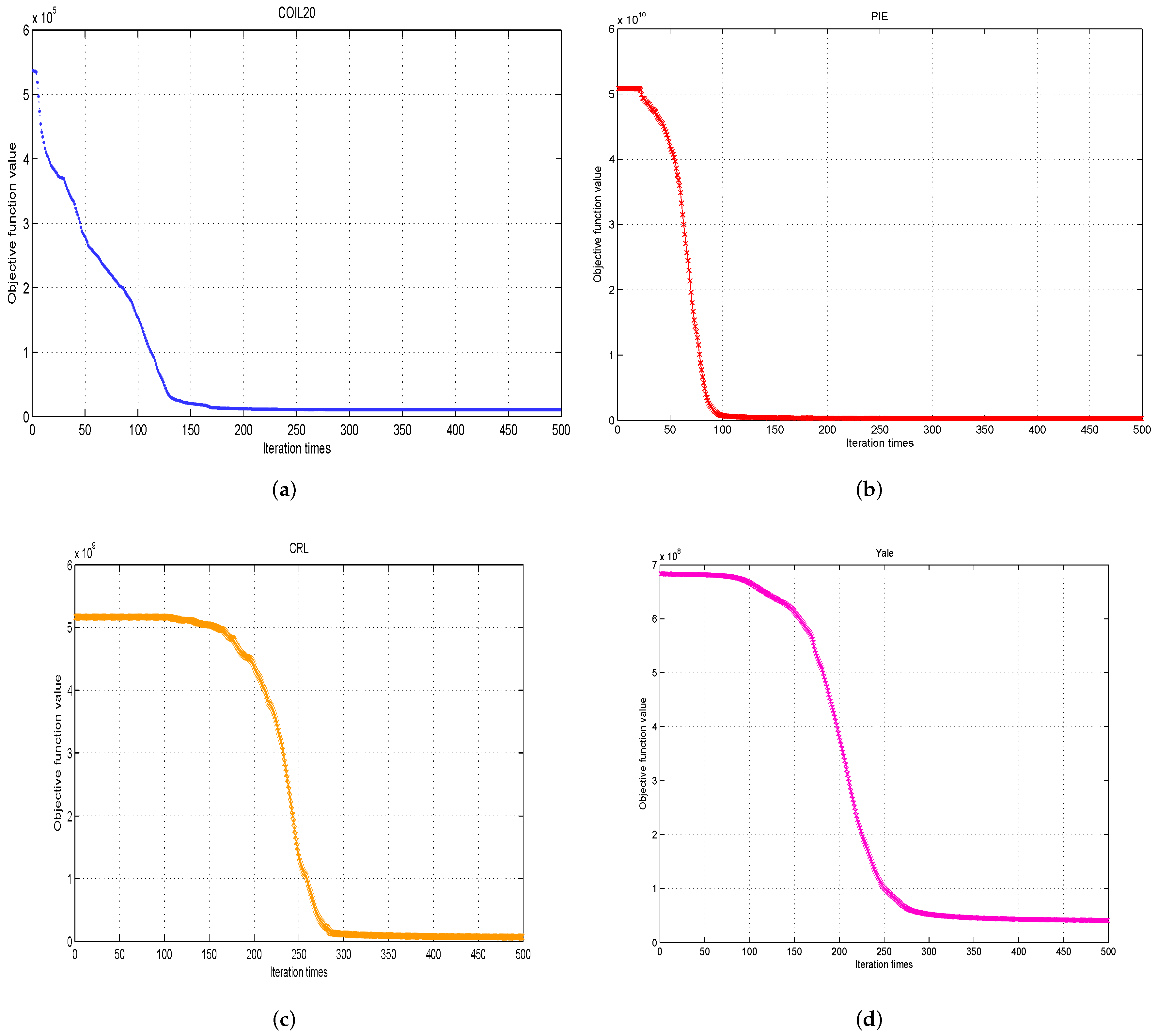
3. Convergence Analysis

In this section, we will give the convergence theorem for Algorithm 1. For the objective function

$$F(X,Y)=\frac{1}{2}{\Vert A-AXY\Vert }_F^2+\frac{\rho }{4}{\Vert X^{T}X-I_p\Vert }_F^2$$

of Problem (4), we first prove that

$$F(X^{(k+1)},Y^{(k+1)})\le F(X^{(k)},Y^{(k)}),$$

where $X^{(k)}$ and $Y^{(k)}$ are the k-th iteration of Algorithm 1, then obtain the limit point as the stationary point of Problem (4). In order to develop this section, we need a lemma.

Lemma 1

([21]). If there exists a function $G(u,u^{{}^{\prime }})$ of $H(u)$ satisfying

$$G(u,u^{{}^{\prime }})\ge H(u),G(u,u)=H(u),$$

(16)

then $H(u)$ is non-increasing under the update rule

$$u^{(k+1)}=arg\underset{u}{min}G(u,u^{(k)}).$$

Here $G(u,u^{{}^{\prime }})$ is called an auxiliary function of $H(u)$ if it satisfies (16).

Theorem 2.

Fixing X, the objective function $F(X,Y)$ is non-increasing, that is

$$\mathit{F}({\mathit{X}}^{(\mathit{k})},{\mathit{Y}}^{(\mathit{k}+\mathit{1})})\le \mathit{F}({\mathit{X}}^{(\mathit{k})},{\mathit{Y}}^{(\mathit{k})}).$$

Proof. 

Set $A=[f_1,f_2,\cdots ,f_m]$ and $Y=(y_1,y_2,\cdots ,y_m)$, then

$${\Vert A-AXY\Vert }_F^2=\sum _{i=1}^m{\Vert f_i-AX{y}_i^{(k)}\Vert }^2.$$

Noting that

$$F(X^{(k)},Y^{(k+1)})=\frac{1}{2}\Vert A-A{X}^{(k)}{Y}^{(k+1)}{\Vert }_F^2+\frac{\rho }{4}{\Vert {(X^{(k)})}^T{X}^{(k)}-I_p\Vert }_F^2,$$

$$F(X^{(k)},Y^{(k)})=\frac{1}{2}\Vert A-A{X}^{(k)}{Y}^{(k)}{\Vert }_F^2+\frac{\rho }{4}{\Vert {(X^{(k)})}^T{X}^{(k)}-I_p\Vert }_F^2,$$

and when X is fixed we can ignore the constant term $\frac{\rho }{4}{\Vert X^{T}X-I_p\Vert }_F^2$, then

$$F(X^{(k)},Y^{(k+1)})\le F(X^{(k)},Y^{(k)})⟺\frac{1}{2}\Vert A-A{X}^{(k)}{Y}^{(k+1)}{\Vert }_F^2\le \frac{1}{2}{\Vert A-A{X}^{(k)}{Y}^{(k)}\Vert }_F^2$$

$$⟺\sum _{i=1}^m\Vert f_i-A{X}^{(k)}{y}_i^{(k+1)}\Vert \le \sum _{i=1}^m\Vert f_i-A{X}^{(k)}{y}_i^{(k)}\Vert ⟺\Vert f_i-A{X}^{(k)}{y}_i^{(k+1)}\Vert \le \Vert f_i-A{X}^{(k)}{y}_i^{(k)}\Vert .$$

If we need to prove $F(X^{(k)},Y^{(k+1)})\le F(X^{(k)},Y^{(k)})$, we must prove that

$$H(y)={1/2\Vert f-AXy\Vert }^2$$

is a nonincreasing function. Noting that $H(y)$ is a quadratic function and its second-order Taylor approximation at $y^{(k)}$ is as follows

$$H(y)=H(y^{(k)})+{(y-y^{(k)})}^T\nabla H(y^{(k)})+1/2{(y-y^{(k)})}^T{\nabla }^{2}H(y^{(k)})(y-y^{(k)}),$$

(17)

where

$$\nabla H(y^{(k)})=-X^{T}Af+X^T{A}^{T}AX{y}^{(k)},$$

and

$${\nabla }^{2}H(y^{(k)})=X^T{A}^{T}AX.$$

Now we will construct a function

$$G(y,y^{(k)})=H(y^{(k)})+{(y-y^{(k)})}^T\nabla H(y^{(k)})+1/2{(y-y^{(k)})}^T\overline{P}(y-y^{(k)}),$$

(18)

where $\overline{P}$ is a diagonal matrix with

$$\begin{array}{c}\hfill {\overline{P}}_{ii}=\left\{\begin{array}{cc}\frac{{(X^T{A}^{T}AX{\overline{y}}^{(k)})}_i+\delta }{{\overline{y}}_i^{(k)}},\hfill & ifi\in I,\hfill \\ 0,\hfill & ifi\notin I.\hfill \end{array}\right.\end{array}$$

$I=\{i\mid y_i^{(k)}>0,\nabla H{(y^{(k)})}_i\ne 0$ or $y_i^{(k)}=0,\nabla H{(y^{(k)})}_i<0\}\triangleq \{i\mid {\overline{y}}_i^{(k)}>0,$$\nabla H{(y^{(k)})}_i\ne 0\}.$

We begin to prove that $G(y,y^{(k)})$ is an auxiliary function of $H(y)$. It is obvious that $G(y,y)=H(y)$ is satisfied; now we prove that the inequality $G(y,y^{(k)})\ge H(y)$ holds. Noting that

$$G(y,y^{(k)})-H(y)=1/2(y-y^{(k)})(\overline{P}-{\nabla }^{2}H(y^{(k)}))(y-y^{(k)})=1/2(y-y^{(k)})(\overline{P}-X^T{A}^{T}AX)(y-y^{(k)}).$$

In fact, we can prove that the matrix $\overline{P}-X^T{A}^{T}AX$ is a positive semi-definite matrix.

Case I.

When $\nabla H(y^{(k)})>0$ or $\nabla H(y^{(k)})<0$ but $y_i^{(k)}>\delta >0$, we have ${\overline{y}}_i^{(k)}=y_i^{(k)}$. For any nonzero vector $z={(z_1,z_2,\cdots ,z_p)}^T\in R^p$, we have

$$\begin{array}{cc}\hfill & z^T(\overline{P}-X^T{A}^{T}AX)z\hfill \\ \hfill & =\sum _{i=1}^p\frac{{(X^T{A}^{T}AX{y}^{(k)})}_i}{{(Y^{(k)})}_i}{z}_i^2+\sum _{i=1}^p\frac{\delta }{{(y^{(k)})}_i}{z}_i^2-\sum _{i=1}^p\sum _{j=1}^p{(X^T{A}^{T}AX)}_{ij}{z}_i{z}_j\hfill \\ \hfill & >\sum _{i=1}^p\frac{{(X^T{A}^{T}AX{y}^{(k)})}_i}{{(y^{(k)})}_i}{z}_i^2-\sum _{i=1}^p\sum _{j=1}^p{(X^T{A}^{T}AX)}_{ij}{z}_i{z}_j\hfill \\ \hfill & =1/2\sum _{i=1}^p\sum _{j=1}^p\frac{{(X^T{A}^{T}AX)}_{ij}{(y^{(k)})}_i}{{(y^{(k)})}_j}{z}_j^2+1/2\sum _{i=1}^p\sum _{j=1}^p\frac{{(Z^T{A}^{T}AX)}_{ji}{(y^{(k)})}_j}{{(y^{(k)})}_i}{z}_i^2-\sum _{i=1}^p\sum _{j=1}^p{(X^T{A}^{T}AX)}_{ij}{z}_i{z}_j\hfill \\ \hfill & =1/2\sum _{i=1}^p\sum _{j=1}^p{(\sqrt{\frac{y_i^{(k)}}{y_j^t}}{z}_j-\sqrt{\frac{y_j^t}{y_i^{(k)}}}{z}_i)}^2{(X^T{A}^{T}AX)}_{ij}\ge 0.\hfill \end{array}$$

The last inequality is true due to the nonnegativity of X, and the data matrix A generally has practical significance, so the elements are usually nonnegative; therefore, we can obtain that the matrix $X^T{A}^{T}AX$ is also a nonnegative matrix. Thus we obtain

$$G(y,y^{(k)})\ge H(y).$$

(19)

Case II.

When $\nabla H(y^{(k)})<0$ and $\delta >y_i^{(k)}>0$, we have ${\overline{y}}_i^{(k)}=\delta$, we can also use the same technique to verify that matrix $\overline{P}-X^T{A}^{T}AX$ is positive semi-definite. According to Lemma 1, we obtain that $H(y)$ is anon-increasing function so $F(X,Y)$ is non-increasing when X is fixed. Therefore, we can obtain

$$F(X^{(k)},Y^{(k+1)})\le F(X^{(k)},Y^{(k)}).$$

(20)

This completes the proof. □

Similarly, we can use the same method to verify that when Y is fixed, the function $F(X,Y)$ is also a non-increasing function. Thus, we have

$$F(X^{(k+1)},Y^{(k)})\le F(X^{(k)},Y^{(k)}).$$

(21)

Consequently, by (20) and (21), we obtain

$$F(X^{(k+1)},Y^{(k+1)})\le F(X^{(k+1)},Y^{(k)})\le F(X^{(k)},Y^{(k)}).$$

(22)

Theorem 3.

The sequence $\left\{(X^{(k)},Y^{(k)})\right\}$ generated by Algorithm 1 converges to the stationary point of Problem 1.

Proof. 

Since $F(X^{(k)},Y^{(k)})$ is a decreasing sequence and it is bounded with the lower bound zero and the upper bound $F(X^{(0)},Y^{(0)})$, and combining Theorem 1, there exist nonnegative matrices $(X^{\ast },Y^{\ast })$ such that

$$\underset{k\ge 0,k\to \infty }{lim}F(X^{(k)},Y^{(k)})=F(X^{\ast },Y^{\ast }).$$

Because of the continuity and monotonicity of the function F, we can obtain

$$\underset{k\ge 0,k\to \infty }{lim}(X^{(k)},Y^{(k)})=(X^{\ast },Y^{\ast }).$$

(23)

Now we will prove the point $\left\{(X^{\ast },Y^{\ast })\right\}$ is the stationary point of Problem 1, that is, we will prove that $\left\{(X^{\ast },Y^{\ast })\right\}$ satisfies the KKT conditions (5). We first prove

$$if{Y}_{ij}^{\ast }>0,then{({\nabla }_{Y}F(X^{\ast },Y^{\ast }))}_{ij}=0,$$

(24)

and

$$if{Y}_{ij}^{\ast }=0,then{({\nabla }_{Y}F(X^{\ast },Y^{\ast }))}_{ij}\ge 0.$$

(25)

Based on the definition of ${\overline{Y}}_{ij}$ in (14)

$${\overline{Y}}_{ij}^{(k)}=max(Y_{ij}^{(k)},\sigma )\mathrm{or}{Y}_{ij}^{(k)},$$

so the sequence $\left\{{\overline{Y}}_{ij}^{(k)}\right\}$ may have two convergent points $Y_{ij}^{\ast }$ or $\sigma$. We set

$${\tilde{Y}}^{\ast }=\underset{k\ge 0,k\to \infty }{lim}{\overline{Y}}^{(k)}.$$

Furthermore, according to (25), we have

$$\underset{k\ge 0,k\to \infty }{lim}(Y_{ij}^{(k+1)}-Y_{ij}^{(k)})=\frac{{\tilde{Y}}_{ij}^{\ast }{[{\nabla }_{Y}F(X^{\ast },Y^{\ast })]}_{ij}}{{[{(X^{\ast })}^T{A}^{T}A{X}^{\ast }{Y}^{\ast }]}_{ij}+\delta }=0.$$

(26)

When $Y_{ij}^{\ast }>0$, we have ${\tilde{Y}}_{ij}^{\ast }>0$; thereby it immediately implies ${\nabla }_{Y}F(X^{\ast },Y^{\ast })=0$ which is consistent with (24). Now we begin to prove (25). If the result is not true, there exists $(i,j)$ such that

$$Y_{ij}^{\ast }=0\mathrm{but}{[{\nabla }_{Y}F(X^{\ast },Y^{\ast })]}_{ij}<0.$$

When k is large enough, we have ${[{\nabla }_{Y}F(X^{(k)},Y^{(k)})]}_{ij}<0$ and

$$\underset{k\ge 0,k\to \infty }{lim}{\overline{Y}}_{ij}^{(k)}={\tilde{Y}}_{ij}^{\ast }=\sigma .$$

Therefore

$$\frac{{\tilde{Y}}_{ij}^{\ast }{[{\nabla }_{Y}F(X^{\ast },Y^{\ast })]}_{ij}}{{[{(X^{\ast })}^T{A}^{T}A{X}^{\ast }{Y}^{\ast }]}_{ij}+\delta }>0,$$

which is a contradiction of (26); hence, (25) holds. (24) and (25) imply that $Y^{\ast }$ satisfies the KKT conditions (5). In a similar way, we can prove that $X^{\ast }$ satisfies the KKT conditions (5). Hence, $(X^{\ast },Y^{\ast })$ is the stationary point of Problem 1. □

4. Numerical Experiments

In this section, we first present a simple example to illustrate that Algorithm 1 is feasible to solve Problem 1, and we apply Algorithm 1 to unsupervised feature selection. We also compare our algorithm with the MaxVar Algorithm [22], the UDFS Algorithm [23] and the MFFS Algorithm [24]. All experiments were performed in MATLAB R2014a on a PC with an Intel Core i5 processor at 2.50 GHz with a precision of $\epsilon =2.22\times {10}^{-16}$. Set the gradient value

$$GV(X,Y)=\Vert {\nabla }_X{F(X,Y)\odot X\Vert }_F^2+{\Vert {\nabla }_{Y}F(X,Y)\odot Y\Vert }_F^2.$$

Due to the KKT conditions (5) we know that if $GV(X,Y)=0$ then $(X,Y)$ is the stationary point of Problem 1. So we use either $GV(X,Y)\le 1.0\times {10}^{-4}$ or the iteration step k has reached the upper limit 500 as the stopping criterion of Algorithm 1.

4.1. A Simple Example

Example 1.

Considering Problem 1 with n = 5, m = 4, p = 3 and

$$A=\left(\begin{array}{cccc}0.6882& 0.0113& 0.6763& 0.3245\\ 0.4984& 0.2828& 0.5696& 0.5210\\ 0.0990& 0.5896& 0.5517& 0.8649\\ 0.2878& 0.1720& 0.9674& 0.9941\\ 0.5381& 0.1701& 0.6284& 0.8385\end{array}\right).$$

Set the initial matrices

$$X^{(0)}=\left(\begin{array}{ccc}0.3474& 0.4812& 0.9596\\ 0.7494& 0.2862& 0.4421\\ 0.9394& 0.5952& 0.9620\\ 0.6681& 0.3364& 0.6764\end{array}\right),Y^{(0)}=\left(\begin{array}{cccc}0.7061& 0.8338& 0.4641& 0.8316\\ 0.9577& 0.1552& 0.2987& 0.5391\\ 0.9399& 0.8304& 0.5233& 0.2598\end{array}\right).$$

We use Algorithm 1 to solve this problem. After 99 iterations, we get the solution of Problem 1 as follows

$$X^{(99)}\approx \left(\begin{array}{ccc}0& 0& 0.9478\\ 0.9764& 0& 0\\ 0& 1.0000& 0\\ 0.0236& 0& 0.0522\end{array}\right),Y^{(99)}\approx \left(\begin{array}{cccc}0.0005& 0.9781& 0.6839& 1.3647\\ 0& 0& 0& 0\\ 1.0662& 0.0966& 1.1570& 0.8467\end{array}\right),$$

and

$$GV(X,Y)=9.8992\times {10}^{-5}.$$

This example shows that Algorithm 1 is feasible to solve Problem 1.

4.2. Application to Unsupervised Feature Selection and Comparison with Existing Algorithms

4.2.1. Dataset

In the next stage of our study, we used standard databases to test the performance of our proposed algorithm. We first describe the four datasets use, the target image is shown in Figure 1, and the characteristics of which are summarized in

Table 1. Database Description.

Dataset	Size	Features	Classes	Data Types
COIL20	1440	1024	20	Object images
PIE	1166	1024	53	Face images
ORL	400	1024	40	Face images
Yale	165	1024	15	Face images

.

1. COIL20 (http://www.cad.zju.edu.cn/home/dengcai/Data/MLData.html (accessed on 1 December 2021)): This dataset contains 20 objects. The images of each object were taken 5 degrees apart as the object was rotated on a turntable, and for each object there are 72 images. The size of each image is $32\times 32$ pixels, with 256 grey levels per pixel. Thus, each image is represented by a 1024-dimensional vector.

2. PIE (http://archive.ics.uci.edu/ml/datasets.php (accessed on 1 December 2021)): This is a face image dataset with 53 different people; for each subject, 22 pictures were taken under different lighting conditions with different postures and expressions.

3. ORL (http://www.cad.zju.edu.cn/home/dengcai/Data/FaceData.html (accessed on 1 December 2021)): This dataset contains ten different images of each of 40 distinct subjects. For some subjects, the images were taken at different times, varying the lighting, facial expressions (open/closed eyes, smiling/not smiling) and facial details (glasses/no glasses). All the images were taken against a dark homogeneous background with the subjects in an upright, frontal position (with tolerance for some side movement).

4. Yale (http://www.cad.zju.edu.cn/home/dengcai/Data/FaceData.html (accessed on 1 December 2021)): This dataset contains 165 grayscale images of 15 individuals. There are 11 images per subject, and they have different facial expressions (happy, sad, surprised, sleepy, normal and wink) or lighting conditions (center-light, left-light, right-light). Using the above four datasets, we input these grayscale images as the initial value A, and then used the initial matrix X and Y so that we could obtain a series of function values through the iterative updating of the algorithm. Then, we were able to obtain four convergence curves for different databases, as shown in Figure 2.

4.2.2. Comparison Methods

1. MaxVar [22]: Selecting features according to the variance of features. The feature with the higher variance than others is more important.

2. UDFS [23]: $l_{2,1}$-norm regularized discriminative feature selection method. This method selects the most distinctive feature through the local discrimination information of data and the correlation of features.

3. MFFS [24]: unsupervised feature selection via matrix factorization, in which the objective function originates from the distance between two subspaces.

4.2.3. Parameter Settings

In our proposed method, the parameter $\rho$ was selected from the set $\{10,{10}^2\cdots ,{10}^9\}$. In the following experiments, we set the value of $\rho$ to be ${10}^4,{10}^9,{10}^8$ and ${10}^7$ for the COIL20, PIE, ORL and Yale databases. The numbers of selected features were taken from $\{20,40,60,\dots ,200\}$ for all datasets. Then, we computed the average value of ACC and NMI when selecting different numbers of features. The maximum iteration number (maxiter) was set to 1000. For the sparsity parameters $\gamma$ and $\lambda$ in UDFS, we set $\gamma =\lambda ={10}^{-5}$. The value of parameter $\rho$ in MFFS was set as ${10}^8$. We set $\sigma =\delta =\epsilon ={10}^{-4}$ in our proposed algorithm. The results of the comparison of MaxVar, UDFS, MFFS and our proposed algorithm are presented in Figure 3 and Figure 4. The following two tables give the average accuracy and normalized mutual information calculated using our proposed algorithm.

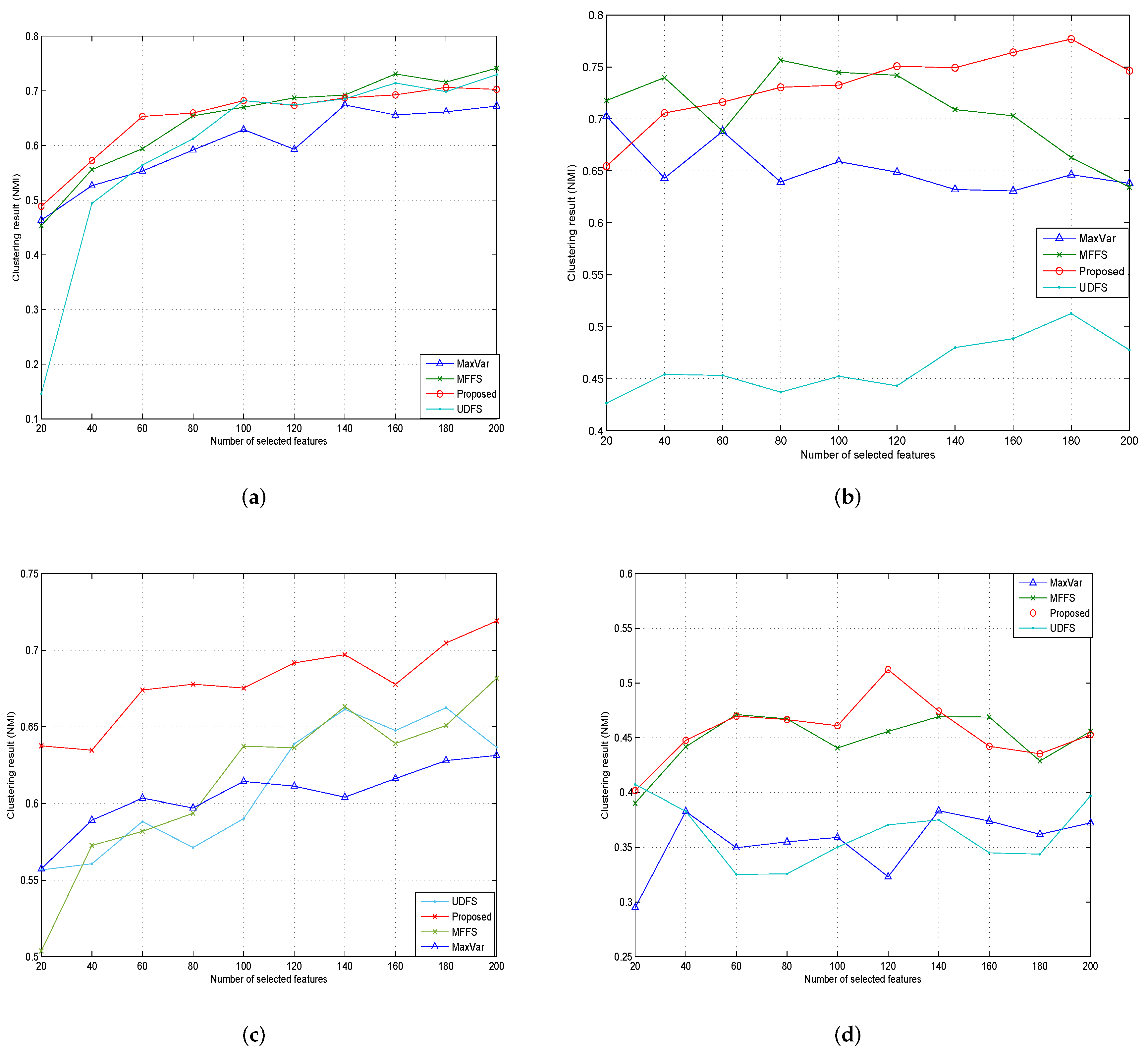
4.2.4. Evaluation Metrics

There are two metrics to measure the results of clustering using the selected features. The accuracy of clustering (ACC) and normalized mutual information (NMI) can be calculated as follows. The value of ACC and NMI scales between 0 and 1, and a high value indicates an efficient clustering result. For every dataset, there are two parts, fea and gnd, the fea data are used to operate the selection, and after clustering one can obtain a clustering label, denoted by $s_i$; gnd is the true label of features denoted by $t_i$, and the ACC can be computed using the clustering label and the true label.

$$\mathrm{ACC}=\frac{{\displaystyle \sum _{i=1}^n}\delta (t_i,map(s_i))}{n},$$

where $\delta (a,b)=1$ if $a=b$; $\delta (a,b)=0$ if $a\ne b$. The $map(·)$ indicates a mapping that permutes the label of clustering result to match the true label as well as possible using the Kuhn–Munkres Algorithm [25]. For two variables P and Q, the NMI is defined in the following form:

$$\mathrm{NMI}(P,Q)=\frac{I(P,Q)}{H(P)H(Q)},$$

where $I(P,Q)$ is the mutual information of P and Q, and $H(P)$ and $H(Q)$ are the entropy of P and Q, respectively.

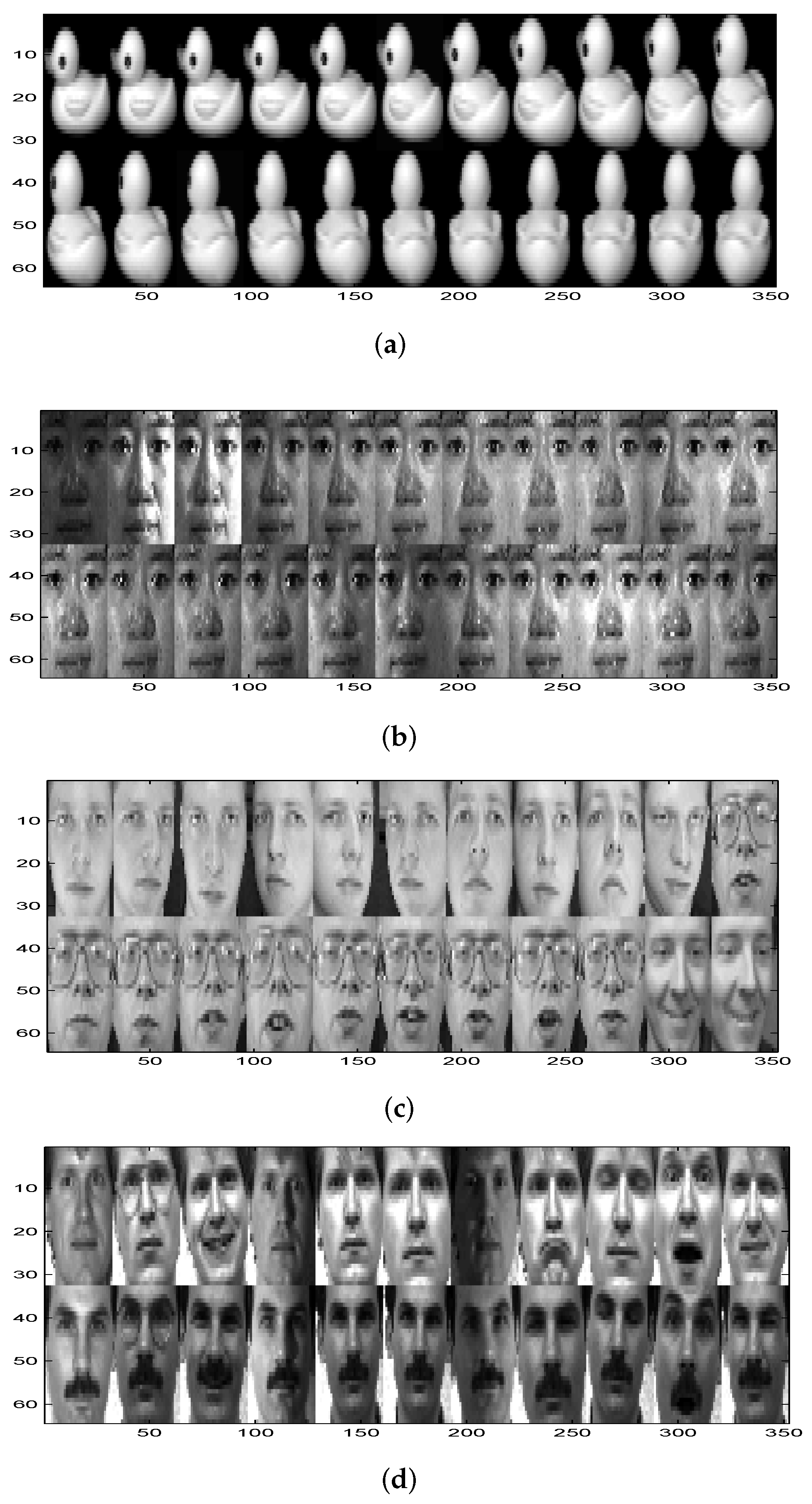
4.2.5. Experiments Results and Analysis

Figure 4 shows the curves of the iteration step and the values of the objective function when Algorithm 1 was run on four datasets. We can see that the objective function value decreases as the iteration step increases. After a finite number of iterations, the objective function value reaches the minimum and tends to be stable.

In

Table 2. Clustering results (average ACC) of different algorithms on different databases.

Dataset	Maxvar	MFFS	UDFS	Algorithm 1
COIL20	0.4881	0.5335	0.5118	0.5404
PIE	0.3865	0.4630	0.2021	0.4799
ORL	0.3770	0.3903	0.4040	0.4798
Yale	0.3049	0.3812	0.2994	0.4000

and

Table 3. Clustering results (average NMI) of different algorithms on different databases.

Dataset	Maxvar	MFFS	UDFS	Algorithm 1
COIL20	0.6020	0.6495	0.6000	0.6518
PIE	0.6527	0.7098	0.4622	0.7322
ORL	0.6052	0.6161	0.6114	0.6790
Yale	0.3557	0.4489	0.3628	0.4563

, we report the best clustering accuracy and the best normalized mutual information, expressed as the number of selected feature changes. In Table 2 and Table 3, we can see that the performance of Algorithm 1 was more effective than that of the MaxVar Algorithm [22], the UDFS Algorithm [23] and the MFFS Algorithm [24] on all data sets, which shows the effectiveness and robustness of our proposed method.

In Figure 3 and Figure 4, we present the clustering accuracy and the normalized mutual information, expressed as the number of selected feature changes. We can see that the performance of MFFS was slightly better than that of Algorithm 1 on COIL20. However, on the other three datasets, Algorithm 1 was relatively more efficient compared with the MaxVar Algorithm [22], the UDFS Algorithm [23] and the MFFS Algorithm [24], especially when the number of selected features was large.

5. Conclusions

The symmetric matrix optimization problem in the area of unsupervised feature selection is considered in this paper. By relaxing the orthogonal constraint, this problem is converted into a constrained symmetric nonnegative matrix optimization problem. An efficient algorithm was designed to solve this problem and its convergence theorem was also derived. Finally, a simple example was given to verify the feasibility of the new method. Some simulation experiments in unsupervised feature selection showed that our algorithm was more effective than the existing methods.

References

1. Lee, D.D.; Seung, H.S. Learning the parts of objects by non-negative matrix factorization. Nature 1999, 401, 788. [Google Scholar] [CrossRef] [PubMed]
2. Smaragdis, P.; Brown, J.C. Non-negative matrix factorization for polyphonic music transcription. In Proceedings of the 2003 IEEE Workshop on Applications of Signal Processing to Audio and Acoustics (IEEE Cat. No.03TH8684), New Paltz, NY, USA, 19–22 October 2003. [Google Scholar]
3. Kim, H.; Park, H. Nonnegative Matrix Factorization Based on Alternating Nonnegativity Constrained Least Squares and Active Set Method. SIAM J. Matrix Anal. Appl. 2008, 30, 713–730. [Google Scholar] [CrossRef]
4. Lin, C. Projected Gradient Methods for Nonnegative Matrix Factorization. Neural Comput. 2007, 19, 2756–2779. [Google Scholar] [CrossRef] [PubMed] [Green Version]
5. Li, X.L.; Liu, H.W.; Zheng, X.Y. Non-monotone projection gradient method for non-negative matrix factorization. Comput. Optim. Appl. 2012, 51, 1163–1171. [Google Scholar] [CrossRef]
6. Han, L.X.; Neumann, M.; Prasad, A.U. Alternating projected Barzilai-Borwein methods for Nonnegative Matrix Factorization. Electron. Trans. Numer. Anal. 2010, 36, 54–82. [Google Scholar]
7. Huang, Y.K.; Liu, H.W.; Zhou, S. An efficient monotone projected Barzilai-Borwein method for nonnegative matrix factorization. Appl. Math. Lett. 2015, 45, 12–17. [Google Scholar] [CrossRef]
8. Gong, P.H.; Zhang, C.S. Efficient Nonnegative Matrix Factorization via projected Newton method. Pattern Recognit. 2012, 45, 3557–3565. [Google Scholar] [CrossRef]
9. Kim, D.; Sra, S.; Dhillon, I.S. Fast Newton-type Methods for the Least Squares Nonnegative Matrix Approximation Problem. In Proceedings of the SIAM International Conference on Data Mining, Minneapolis, MN, USA, 26–28 April 2007. [Google Scholar]
10. Zdunek, R.; Cichocki, A. Non-negative matrix factorization with quasi-newton optimization. In Proceedings of the International Conference on Artificial Intelligence and Soft Computing, Zakopane, Poland, 25–29 June 2006. [Google Scholar]
11. Abrudan, T.E.; Eriksson, J.; Koivunen, V. Steepest descent algorithms for optimization under unitary matrix constraint. IEEE Trans. Signal Process. 2008, 56, 1134–1147. [Google Scholar] [CrossRef]
12. Abrudan, T.E.; Eriksson, J.; Koivunen, V. Conjugate gradient algorithm for optimization under unitary matrix constraint. Signal Process. 2009, 89, 1704–1714. [Google Scholar] [CrossRef]
13. Absil, P.A.; Baker, C.G.; Gallivan, K.A. Trust-Region methods on riemannian manifolds. Found. Comput. Math. 2007, 7, 303–330. [Google Scholar] [CrossRef]
14. Savas, B.; Lim, L.H. Quasi-Newton methods on grassmannians and multilinear approximations of tensors. SIAM J. Sci. Comput. 2010, 2, 3352–3393. [Google Scholar] [CrossRef]
15. Wen, Z.W.; Yin, W.T. A feasible method for optimization with orthogonality constraints. Math. Program. 2013, 142, 397–434. [Google Scholar] [CrossRef] [Green Version]
16. Lai, R.J.; Osher, S. A splitting method for orthogonality constrained problems. J. Sci. Comput. 2014, 58, 431–449. [Google Scholar] [CrossRef]
17. Chen, W.Q.; Ji, H.; You, Y.F. An augmented lagrangian method for l1-regularized optimization problems with orthogonality constraints. SIAM J. Sci. Comput. 2016, 38, 570–592. [Google Scholar] [CrossRef] [Green Version]
18. Han, D.; Kim, J. Unsupervised Simultaneous Orthogonal basis Clustering Feature Selection. In Proceedings of the IEEE Conference on Computer Vision and Pattern Recognition, Boston, MA, USA, 7–15 June 2015. [Google Scholar]
19. Du, S.Q.; Ma, Y.D.; Li, S.L. Robust unsupervised feature selection via matrix factorization. Neurocomputing 2017, 241, 115–127. [Google Scholar] [CrossRef]
20. Yi, Y.G.; Zhou, W.; Liu, Q.H. Ordinal preserving matrix factorization for unsupervised feature selection. Signal Process. Image Commun. 2018, 67, 118–131. [Google Scholar] [CrossRef]
21. Lee, D.D.; Seung, H.S. Algorithms for non-negative matrix factorization. In Proceedings of the International Conference on Neural Information Processing Systems, Vancouver, BC, Canada, 3–8 December 2001. [Google Scholar]
22. Lu, Y.J.; Cohen, I.; Zhou, X.S.; Tian, Q. Feature selection using principal feature analysis. In Proceedings of the 15th ACM International Conference on Multimedia, Augsburg, Germany, 24–29 September 2007. [Google Scholar]
23. Yang, Y.; Shen, H.T.; Ma, Z.G. l21-norm regularized discriminative feature selection for unsupervised learning. In Proceedings of the Twenty-Second International Joint Conference on Artificial Intelligence, Barcelona, Spain, 16–22 July 2011. [Google Scholar]
24. Wang, S.P.; Witold, P.; Zhu, Q.X. Subspace learning for unsupervised feature selection via matrix factorization. Pattern Recognit. 2015, 48, 10–19. [Google Scholar] [CrossRef]
25. Lovász, L.; Plummer, M.D. Matching Theory, 1st ed.; Elsevier Science Ltd.: Amsterdam, The Netherlands, 1986. [Google Scholar]
Figure 1. Some images from different databases. (a) COIL20, (b) PIE, (c) ORL, (d) Yale.
Symmetry 14 00462 g001
Figure 2. Clustering results (ACC) of different feature selection algorithms. (a) COIL20, (b) PIE, (c) ORL, (d) Yale.
Symmetry 14 00462 g002
Figure 3. Clustering results (NMI) of different feature selection algorithms. (a) COIL20, (b) PIE, (c) ORL, (d) Yale.
Symmetry 14 00462 g003
Figure 4. The convergence curves of the proposed approach on four different databases. (a) ρ = 10 4 , (b) ρ = 10 9 , (c) ρ = 10 8 , (d) ρ = 10 7 .
Symmetry 14 00462 g004