Abstract
Solving polynomial equations inevitably faces many severe challenges, such as easily occupying storage space and demanding prohibitively expensive computation resources. There has been considerable interest in exploiting the sparsity to improve computation efficiency, since asymmetry phenomena are prevalent in scientific and engineering fields, especially as most of the systems in real applications have sparse representations. In this paper, we propose an efficient parallel hybrid algorithm for constructing a Dixon matrix. This approach takes advantage of the asymmetry (i.e., sparsity) in variables of the system and introduces a heuristics strategy. Our method supports parallel computation and has been implemented on a multi-core system. Through time-complexity analysis and extensive benchmarks, we show our new algorithm has significantly reduced computation and memory overhead. In addition, performance evaluation via the Fermat–Torricelli point problem demonstrates its effectiveness in combinatorial geometry optimizations.
1. Introduction
As a basic tool in computer algebra and a built-in function of most computer algebra systems, the notion of a resultant is widely used in mathematical theory. A resultant is not only of significance to computer algebra [1], but also plays an important role in biomedicine [2], image processing [3], geographic information [4], satellite trajectory control [5], information security [6] and other scientific and engineering fields [7,8]. The most widely used techniques for solving polynomial systems are Sylvester and Dixon resultants. For example, applying a Dixon resultant to algebraic attacks can quickly solve multivariate polynomial quadratic equations over finite fields. Although these resultant techniques have been extensively studied and improved, they still face many severe challenges regarding their easy occupation of storage space and demand for prohibitively expensive computation resources.
Specifically, a successive Sylvester elimination technique has a shortcoming over a multivariate resultant in that the performance of successive resultant computations is very sensitive to the ordering of variables. Human intervention is required to determine the most efficient ordering, and so they are not automatic methods [9]. Inappropriate choices may cause the extreme intermediate expression to swell, consequently running out of memory before accomplishment [10]. In fact, this method is very inefficient, with the number of variables increasing. Moreover, this technique performs elimination variable by variable, which is inherently sequential.
In contrast, in most cases, the Dixon method is more efficient for directly computing resultant without eliminating variables one at a time. However, it is generally known that the entries of the Dixon matrix are more complicated than the entries of other resultant matrices. As a promising scheme, the fast recursive algorithm of the Dixon matrix (FRDixon for short) [11,12,13,14,15,16] can greatly improve the computation efficiency of the Dixon matrix. Recently, its effectiveness has been analyzed in detail and proven by [16]. Nevertheless, the size of the Dixon matrix and computational complexity by FRDixon explode exponentially as the number of variables increases. If the size of the Dixon matrix is relatively large, it directly leads to difficulty computing the final resultant.
To sum up, it is difficult to overcome such difficulties mentioned above, whatever the choices of resultants. Notice that the conventional resultants resort to general methods for solving polynomial systems. From another point of view, if we can make use of the features of given systems to design customized algorithms for constructing resultant matrices or computing resultants [10], instead of general-purpose methods, it can be expected that we can obtain a targetable method to solve some intractable problems efficiently. Therefore, the main objective of this article is to make use of the sparsity of systems and advantages of prevailing resultants to design a more suitable scheme according to the features of different systems.
Symmetry/asymmetry phenomena are prevalent in scientific and engineering fields. In computer algebra, especially most problems which arise in geometry, we observe the fact that in the real polynomial systems, variables always do not stand uniformly (i.e., with asymmetry features), such as the three combinatorial geometry problems posed in [10] for Heron’s formula in three and four dimensions [17], the problem of mapping of the topographical point to the standard ellipsoid [4], the Fermat–Torricelli point problem on a sphere with an Euclidean metric [18] and bifurcation points of the logistic map [17,19,20]. As we know, in the last decade, there has been considerable interest in employing sparsity to find the solutions in various fields, since most of the systems in real applications actually have sparse representations, such as finding sparse and low-rank solutions [21], parallel GCD algorithm for sparse multivariate polynomials [22], estimating the greatest common divisor (GCD) with sparse coefficients of noise-corrupted polynomials [23] and sparse multivariate interpolation [24].
However, researchers in symbolic computation mainly consider designing the methods to solve an arbitrary given polynomial system and are not aware of such sparse scenarios. In fact, similar studies on sparsity in other fields can go on in the field of solving polynomial systems. In this paper, we propose a new approach to construct a Dixon matrix for solving polynomial equations with sparsity. Through time-complexity analysis and extensive benchmarks, we show our new algorithm has significantly reduced computation and memory overhead.
1.1. Contributions
Our method is combined with Sylvester resultant and fast recursive algorithm FRDixon. It can be partitioned into two phases. In the first phase, we make use of the sparsity of systems to obtain a smaller polynomial system in fewer variables via a Sylvester resultant with fewer computational efforts. In the next step, we consider the multivariate algorithm FRDixon. Since the computational complexity of FRDixon exponentially depends on the number of variables, consequently, via Sylvester resultant elimination, the exported system with fewer variables than operated by FRDixon is more effective than single FRDixon that operates the original system directly. The idea is the genesis of our algorithm employing the Sylvester resultant and FRDixon simultaneously.
The main contributions of this paper are as follows.
- We take advantage of the sparsity of the system and present a heuristic strategy to determine the most effective elimination ordering and remove part of the variables via Sylvester resultant.
- We propose a method to improve the fast recursive algorithm of the Dixon matrix, which leads to reduced time and parallelism available.
- We present a hybrid algorithm employing the methods of 1 and 2 to overcome some computation problems arising in successive Sylvester resultant computations and FRDixon separately. Meanwhile, we apply parallel computation to speed up these two elimination processes.
- We implement our hybrid algorithm and parallel version on Maple. Through time-complexity analysis and extensive random benchmarks, we show our new algorithm has significantly reduced computation and memory overhead in the cases of systems with sparsity. In addition, performance evaluation via the Fermat–Torricelli point problem on sphere with Euclidean metric demonstrates our algorithm’s effectiveness in terms of the real combinatorial geometry optimization problems.
1.2. Related Work
It is well known that successive Sylvester resultant computations can be used to settle the problem of elimination of variables from a multivariate polynomial system to obtain a smaller polynomial system in fewer variables. Implementations of Sylvester resultants are supported in most of the computer algebra systems. With respect to so-called multivariate resultants, A.L. Dixon [25] proposed a method to simultaneously eliminate variables from multivariate systems, aiming at solving the polynomial equations system by constructing a Dixon matrix and computing its determinant.
Since then, Sylvester and Dixon approaches have been generalized and improved (see [9,11,12,16,17,20,26,27,28,29,30,31,32,33,34]). In [26], using the Cholesky decomposition, Zhi et al. proposed a method to compute the Sylvester resultant and reduced the time complexity to , where and r represent the size and numerical rank of the Sylvester matrix, respectively. Kapur et al. [29] extended Dixon’s method for the case when Dixon matrix is singular and successfully proved many non-trivial algebraic and geometric identities. In order to improve the efficiency of computing the Dixon resultant, several methods came into existence, such as the Unknown-Order-Change [30], Fast-Matrix-Construction method [9,31], Corner-Cutting method [32], etc. Zhao et al. [11,12] extended Chionh’s algorithm [31] to the general case of polynomial equations in n variables by n-degree Sylvester resultant, and proposed the FRDixon algorithm, which initially constructed the Dixon matrix of nine Cyclic equations. In 2017, Qin et al. [16] gave a detailed analysis of the computational complexity of Zhao’s recurrence formula setting and applied parallel computation to speed up the recursive procedure [33,34]. To deal with the determinant raised in the Dixon matrix which is too large to compute or factor, some heuristic acceleration techniques were raised to accelerate computation in certain specific cases [17,20].
1.3. Organization
The rest of this article is organized as follows. Section 2 reviews the successive Sylvester resultant computations method and the FRDixon algorithm. In Section 3, a parallel hybrid algorithm which combines the Sylvester resultant and modified FRDixon is developed. Section 4 analyzes the time complexity of our proposed algorithm and conducts a series of numerical experiments. Three sets of random instances and one detailed example are presented to illustrate the application of our method. Finally, a conclusion is reported.
2. Review of Elimination Techniques
In this section, we first review the definition of a Sylvester resultant, which serves as the basis of successive Sylvester resultant computations for solving a system of polynomial equations. Then, we describe the fast recursive algorithm for construction of a Dixon matrix (FRDixon) [11].
All the discussions are stated for a general field , where denotes the set of variables and denotes the set of parameters not belonging to X. Consider a system of polynomial equations
in n variables and a number of coefficients , where is the degree of the polynomial with respect to . The objective is to construct the resultant matrix of polynomial equation system (1).
2.1. Elimination via Sylvester Resultant
In this subsection, we introduce the elimination process variable by variable based on the Sylvester resultant. The classical Sylvester resultant is used to the elimination of systems of two polynomials in one variable. Consider the polynomials f and g:
where and are the degrees of polynomials f and g in x, respectively. Recall that the Sylvester matrix of f and g in x is the matrix of the form
and the resultant of f and g in x is defined as the determinant of matrix S.
Let represent the Sylvester resultant of the polynomial and in . By computing the Sylvester resultant of and other polynomials with respect to , respectively, we obtain the system denoted by
which contains n equations in variables , i.e., the variable is removed from the original system (1). This procedure may be repeated until we have determined the sequence of polynomial systems , . Obviously, the above elimination procedure yields the final resultant for system (1).
Similar to the procedure above, we can eliminate in any order by successive Sylvester resultant computations and finally have a resultant in variable . In the worst cases, this method requires times Sylvester resultant computations.
2.2. Fast Recursive Algorithm of the Dixon Matrix (FRDixon)
We now give the key technique of the fast recursive algorithm for constructing the Dixon matrix in [11]. To avoid the computation of polynomial division, the technique of truncated formal power series (see [31]) is employed in the FRDixon algorithm.
Let be the polynomial in y. It is obvious that when . Therefore, the quotient is a polynomial in y. We denote by series form . Hence,
here is taken as zero. Since the powers of x of the second term are all negatives, the left side of Equation (2) is a polynomial if, and only if, the second term of the right side in (2) is equal to zero. Hence, the equation
holds.
The FRDixon algorithm is based on the following ideas: employing the technique of truncated formal power series for reducing the Dixon matrix construction problem into a set of sub-Dixon matrix construction problems with fewer variables, and using the Sylvester resultant matrix and the Dixon matrix with () variables to represent the Dixon matrix with k variables via matrix block computation. A recursive process for constructing the Dixon matrix is then proposed. For more details, one can refer to [11,12,16].
3. A Hybrid Algorithm for Constructing a Dixon Matrix
In this section, we will propose a new method to construct the Dixon matrix. Additionally, our proposed scheme is a parallel hybrid approach utilizing both the Sylvester resultant and the modified FRDixon algorithm, and making our algorithm applicable in either random polynomial systems or problems in reality.
The time complexity of our algorithm for construction of the Dixon matrix of defined by (1) is (numerical type determinant) or (symbolic type determinant), where is the degree bound of the polynomial, denotes the maximum degree of in all polynomials , n denotes the number of variables and t denotes the number of variables in the polynomial system after the Sylvester resultant eliminates some variables. See Section 4.1 for details of the proof. In comparison, our method is more efficient than the existing methods for solving sparse polynomial systems.
Our method can be partitioned into two phases. In the first phase, we eliminate part of variables by Sylvester resultant from the original system, and then in the second phase, we construct the resultant matrix of the system derived from the first phase by a variant version of FRDixon.
3.1. Sylvester Elimination by Heuristic Strategy
A successive Sylvester elimination technique requires computations to remove a variable for a non-sparse system. If the sparse condition is satisfied, we can obtain a smaller system with the least computation costs.
In this subsection, we describe a heuristic strategy to determine which variable should be eliminated first. According to the degrees of this variable in each polynomial of the system, we can give the optimal combinational relationships of polynomials for removing it by Sylvester resultant.
If there are some variables only appearing in a few equations of system (1), the computation cost of eliminating such variables from (1) will be relatively small. In such a case, our approach to decide the elimination ordering and then remove them via Sylvester resultant in the first phase is fairly straightforward.
Let represent whether the variable appears in polynomial . That is,
For each , we compute the sum of for denoted by
Assume denotes the first variable to be eliminated from system (1). Then, for , it satisfies
means the maximum degree of in all polynomials . Once is picked, we move to adjust the ordering of . Let for be the order of after rearrangement. We require that if , then . At this stage, the ordering of polynomials is rearranged according to the degree ; we denote the rearrangement system by .
From now on, the technique of successive Sylvester resultant computations is operated on the newly adjusted system . Assume the first l polynomials do not contain variable . In such a case, we only need to eliminate from the last polynomials by computing the resultants . Let
Then, a new polynomial system
with variables is obtained.
We can proceed with eliminating a variable from (6) in way similar to that shown above. This approach in the first phase is illustrated in Example 1.
Example 1.
Given a system
we want to eliminate a variable with the least computation cost. For each variable , count the number of times of appearing in according to (4). We find that the minimum of is 2 corresponding to . Therefore, is chosen to be eliminated first and can be rearranged by . The rearranged system is
Since does not appear in and , eliminating by computing , we obtain the system of 3 equations and 2 variables as
Note that if is chosen to be eliminated first instead of , this yields a much larger system:
Remark 1.
An attractive feature of the hybrid algorithm is that it reflects the polynomial sparsity of the system. Hence, our overall algorithm is sensitive to the sparsity of variables appearing in its original representation of a given system.
3.2. Construction of Dixon Matrix by Improved FRDixon
At this stage, assume that we have eliminated variables via successive Sylvester elimination techniques by making use of a heuristic strategy. The derived system is denoted by ,
where denotes the degree of variable in . denotes the coefficients of monomial.
The rest of the work constructs a Dixon matrix using an improved FRDixon algorithm. In our new version, we replace the computations of the product of Sylvester matrix and block matrix to the sum of products of a set of matrices with smaller size, which leads to reduced time and parallelism available.
Specifically, is expressed by
where is exacted from the coefficients of polynomials . The order of is .
The block matrix is constructed by
where denotes the l-row of defined by (14). The order of is .
In the original version, and are computed, respectively. The improved algorithm considers as the sum of products of a set of ; that is
where is the matrix defined by (13).
In our theoretical analysis in Theorem 1 with an improved FRDixon algorithm, we find that the key advantages to this matrix decomposition are as follows.
- There is no need to construct matrix for explicitly. This is in contrast with the original FRDixon, which requires computing matrix from one by one.
- Compared to , matrix with a smaller size can be computed independently and, consequently, has the advantage of working in parallel.
- Decomposition of (8) leads to reduced time.
Based on above analysis, we now give a description of Algorithm 1.
| Algorithm 1: Improved FRDixon algorithm. |
Input: : multivariate polynomial system with equations and t variables . Output: : Dixon matrix of . Step 1. (Decompose Dixon polynomial into a set of sub-Dixon polynomials.) By introducing the new variables to , we form the Dixon polynomial defined as
Step 2. (Express the Dixon polynomial in terms of Dixon matrix.) Deduce the recursive formula for Dixon matrix, express sub-Dixon polynomials in Dixon matrix from Step 3. (Construct the matrix
.) Extract the coefficients of to construct the matrix Step 4. (Construct the matrix .) Compute the sum of sub-Dixon matrices corresponding to sub-Dixon polynomials in (12), denoted by
Step 5. (Compute .) Step 6. (Construct using .) From the evaluations of for and , construct Dixon matrix,
|
3.3. The Parallel Hybrid Algorithm
In Section 3.1 and Section 3.2, we describe the two phases involved in our hybrid algorithm. Now, the overall algorithm is presented.
Remark 2.
The Algorithm 2 presented corresponds to our sequential implementation. Further parallel is available. In particular,
- In step 2, once is determined to be eliminated, we simultaneously have at our disposal the computations . Hence, can be obtained in parallel.
- In step 3 and step 4, and can each be obtained independently. Hence, the computations of and can be carried out in parallel.
- In step 5, once and are known to us, we can compute immediately. Hence, the initialization of can be performed in parallel.
- In step 6, recursive operation is carried out on each anti-diagonal line as can also be performed in parallel.
| Algorithm 2: Hybrid algorithm. |
Input: : multivariate polynomial system with equations and n variables over . Output: : Dixon matrix of . Step 1. (Select variable to be eliminated from by applying heuristic scheme.) Select the variable to be eliminated according to (5). Then, rearrange the polynomial in terms of the degrees of in . Denote the rearranged polynomial system as . Step 2. (Eliminate from .) Assume the polynomials do not contain variable . Eliminate from by Sylvester resultant: Step 3. (Construct the matrix .) fordo for do Construct the by (13) in Algorithm 1. end k for; endifor; Step 4. (Construct the matrix .) fordo for do Construct the by (14) recursively in Algorithm 1. end k for; endjfor; Step 5. (Initialize the elements of .) From step 3 and step 4, compute the product of by (8) and then initialize the elements of . Step 6. (Construct the .) Observing (15), we find that the following relationship holds, |
Our method exploits the sparsity in variables of the system and introduces heuristics strategy. Parts of the variables are chosen to be eliminated from the original system via successive Sylvester resultant computations. Next, the exported system with fewer variables is operated by improved FRDixon. Meanwhile, these two elimination processes can be paralleled.
4. Analysis and Evaluation
We first analyze the time complexity of the hybrid algorithm in Section 4.1, and then evaluate the performance of our algorithm. In Section 4.2, we discuss implementations in random instances. Section 4.3 reports on our approach in a real problem. The effectiveness and practicality of our method are illustrated in these examples.
4.1. Time Complexity Analysis
We now give the sequential complexity of the hybrid algorithm in terms of the number of arithmetic operations, and use big-O notation to simplify expressions and asymptotically estimate the number of operations algorithm used as the input grows.
Theorem 1.
The time complexity of the hybrid algorithm (Algorithm 2) for construction of Dixon matrix of defined by (1) is (numerical type determinant) or (symbolic type determinant).
Proof.
Similar to the framework of a hybrid algorithm, we partition two phases to analyze the sequential complexity of our new method.
In the first phase, we consider successive Sylvester resultant computations. The most expensive component of this part is to compute a set of Sylvester resultants. It can be shown that evaluation of a numerical determinant using row operations requires about arithmetic operations ([35]). If symbolic determinant needs to be computed, a cofactor expansion requires over multiplications in general. Suppose that variables are eliminated in the whole successive Sylvester resultant computations. When the ith elimination process is performed, we let for denote the number of Sylvester resultant computations and denote the degree bound of polynomials.
In terms of the complexity of determinant computation, the first phase requires arithmetic operations for numerical determinant or arithmetic operations for the symbolic determinant. Hence, the complexity of this part is or using big-O notation.
In the second phase, we consider improved FRDixon for system (7). The main cost is calculation of (8). Each of these ’s requires
multiplications and
additions. The calls to compute cost
multiplications and
additions. The can be constructed in additions using the method given in (16). Hence, the complexity of improved FRDixon is
multiplications and
additions, where . If we use big-O notation, the complexity of improved FRDixon is .
Hence, the complexity of hybrid algorithm is for numerical type or for symbolic type. □
4.2. Random Systems
To compare the performance of our hybrid algorithm, successive Sylvester resultant elimination method and FRDixon ([11,16]), we have implemented these algorithms on three benchmark sets with different sizes. All timings reported are in CPU seconds and were obtained using Maple 18 on Intel Core i5 3470 @ 3.20 GHz running Windows 10, involving basic operations such as matrix multiplication and determinant calculations.
4.2.1. Timings
Each polynomial of systems S1–S30 in Table 1, Table 2 and Table 3 is generated at random using the Maple command ‘randpoly’. To guarantee the sparsity of the system, remove one variable randomly from each polynomial in every system of S1–S30. One hundred instances are contained in each system and the average running time is reported. The timings for columns 4, 5 and 6 of Table 1, Table 2 and Table 3 are for the successive Sylvester resultant elimination method (SylRes for short), FRDixon and hybrid algorithm (Hybrid for short), respectively. To better assess the parallel implementation of our algorithm, we report timings and speed-ups for four cores listed in column 7 in Table 1, Table 2 and Table 3. ’—’ indicates that the program went on for more than 2000s, or ran out of space.
Benchmark
This set of benchmarks consists of 10 groups of systems. Every system of S1–S10 contains five polynomial equations in four variables.
The data in Table 1 show that for systems S1–S10, our new algorithm has a better performance compared to FRDixon. For systems S1–S4, SylRes has fewer timings than the hybrid algorithm. As terms and degrees increase, systems become more complex. Our hybrid algorithm is superior to SylRes. Considering test instances S9 and S10, we tried successive resultant computations using the existing implementations of Sylvester’s resultant in Maple for various variable orderings, but most of the time, the computations run out of memory. We also tried to compute Dixon matrix by FRDixon. The program ran for up to 2000s in these examples.

Table 1.
Benchmark : variables = 4.
Table 1.
Benchmark : variables = 4.
| System | Term | Degree | Average Time (s) | |||
|---|---|---|---|---|---|---|
| SylRes | FRDixon | Hybrid | Hybrid (in Parallel) | |||
| S1 | 4 | 2 | 0.43 | 11.575 | 2.283 | 0.771 |
| S2 | 5 | 2 | 0.93 | 19.274 | 2.673 | 0.879 |
| S3 | 6 | 3 | 11.40 | 216.115 | 40.398 | 11.481 |
| S4 | 7 | 3 | 36.02 | 234.975 | 49.641 | 13.264 |
| S5 | 8 | 4 | 234.51 | 558.974 | 94.813 | 24.813 |
| S6 | 9 | 4 | 265.42 | 568.757 | 105.221 | 28.952 |
| S7 | 10 | 5 | 1469.08 | 906.224 | 287.381 | 73.475 |
| S8 | 11 | 5 | 1564.15 | 921.901 | 297.517 | 76.837 |
| S9 | 12 | 6 | — | — | 764.242 | 195.073 |
| S10 | 13 | 6 | — | — | 773.361 | 197.019 |
Benchmark
This set of systems differs from the first benchmark in that the degree of each polynomial is set to be four in the second set. The number of terms and variables varies from small to large.
In the experimentation of benchmark in Table 2, we found that our new hybrid algorithm is faster than FRDixon for computing the Dixon matrix. Notice that when the number of variables increases up to 7 and the terms of polynomials reach 12 or more, the FRDixon was not successfully terminated after 2000s. There were similar results for benchmark . Successive Sylvester resultant computations cost less than our method in simple systems S11 and S12. However, for complicated systems, the successive technique shows its inefficiency.
Table 2.
Benchmark : degrees = 4.
Table 2.
Benchmark : degrees = 4.
| System | Term | Variable | Average Time (s) | |||
|---|---|---|---|---|---|---|
| SylRes | FRDixon | Hybrid | Hybrid (in Parallel) | |||
| S11 | 4 | 3 | 0.23 | 6.391 | 0.507 | 0.187 |
| S12 | 5 | 3 | 0.21 | 5.330 | 0.847 | 0.223 |
| S13 | 6 | 4 | 203.74 | 524.672 | 89.325 | 23.492 |
| S14 | 7 | 4 | 219.53 | 533.013 | 98.321 | 26.398 |
| S15 | 8 | 5 | 564.12 | 760.180 | 279.945 | 70.447 |
| S16 | 9 | 5 | 596.09 | 781.112 | 299.864 | 76.106 |
| S17 | 10 | 6 | 1759.25 | 1265.803 | 594.381 | 151.093 |
| S18 | 11 | 6 | — | 1301.021 | 617.829 | 155.479 |
| S19 | 12 | 7 | — | — | 1359.986 | 346.983 |
| S20 | 13 | 7 | — | — | 1505.042 | 382.271 |
Benchmark
This set of benchmarks consists of 10 groups of systems of terms polynomial equations with varying numbers of variables and degrees. See Table 3. As analysis of the complexity of the hybrid algorithm, the number of arithmetic operations is mainly affected by variables and degrees. With the increase in these two parameters, three algorithms need more computation time for completion. Facing intractable systems S27–S30, SylRes and FRDixon are both powerless.
In all experiments listed in Table 1, Table 2 and Table 3, our hybrid algorithm always takes advantage of the sparsity of a given system and combines successive Sylvester resultant computations with improved FRDixon. The average running time is never more than the original FRDixon. Except for some “simple” instances, the new algorithm has a better performance compared to successive Sylvester resultant computations.
Table 3.
Benchmark : terms = 6.
Table 3.
Benchmark : terms = 6.
| System | Degree | Variable | Average Time (s) | |||
|---|---|---|---|---|---|---|
| SylRes | FRDixon | Hybrid | Hybrid (in Parallel) | |||
| S21 | 2 | 3 | 0.02 | 2.640 | 0.207 | 0.072 |
| S22 | 3 | 3 | 0.12 | 5.639 | 0.440 | 0.134 |
| S23 | 3 | 4 | 11.01 | 223.527 | 34.568 | 9.007 |
| S24 | 4 | 4 | 125.03 | 516.969 | 87.380 | 22.043 |
| S25 | 4 | 5 | 532.52 | 727.617 | 271.239 | 69.971 |
| S26 | 5 | 5 | 844.64 | 1106.289 | 478.947 | 122.307 |
| S27 | 5 | 6 | — | — | 851.086 | 215.152 |
| S28 | 6 | 6 | — | — | 987.602 | 249.005 |
| S29 | 6 | 7 | — | — | 1823.056 | 460.764 |
| S30 | 7 | 7 | — | — | 1909.443 | 483.125 |
4.2.2. Matrix Dimension
According to the definition of the resultant (determinant of resultant matrix), one can notice that the dimension of resultant matrix is the key factor affecting the computational complexity on the target resultant. In order to compare the matrix dimension generated by FRDixon and the hybrid algorithm, we record the matrix sizes of systems S1–S30, as shown in Table 4, Table 5 and Table 6.
Table 4.
Matrix dimensions corresponding to systems in Table 1.
Table 5.
Matrix dimensions corresponding to systems in Table 2.
Table 6.
Matrix dimensions corresponding to systems in Table 3.
4.3. Real Problems
In order to measure the comprehensive performance of the hybrid algorithm in the real problems, we implement our new algorithm on an open optimization problem in combinatorial geometry.
Given a spherical triangle whose length of sides are a, b and c, respectively, the problem is to find a point P on the sphere such that the sum of distances L between the point P and the vertexes of reaches the minimum.
As illustrated in Figure 1, let , , , , , and . All distances are measured by an Euclidean metric. If we can find the relationship between a, b, c and L, the original minimum problem is solved.
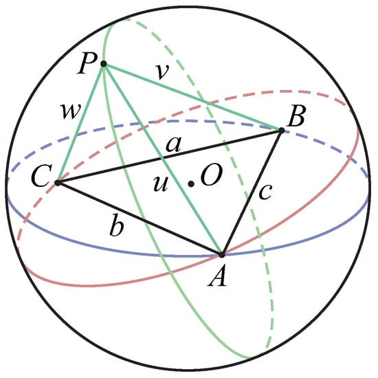
Figure 1.
A triangle ABC on the sphere and their Fermat–Torricelli point P.
By applying the Lemma in [36] and the compactness of the sphere, we can prove that a point P on sphere is such that the Cayley–Menger determinant equals to zero. That is, the distances between the center point O of the sphere and A, B, C, P should satisfy
Now, we transform the relationship between a, b, c and L into an optimization problem of the following form
Consequently, the Fermat–Torricelli point P on the sphere is such that the polynomial system
where
From (17)–(20), we obtain the polynomial system
It is easy to know that this geometry problem is equivalent to solving the polynomial system (21) with five equations and four variables.
We first report the result that (21) solved by successive Sylvester resultant computation techniques. The order of elimination is , u, v and w. Starting with computing and , the variable is eliminated from (21),
This is followed by computing
and
to eliminate u and v, respectively. Finally, w is eliminated by computing
It was found that the elimination process of could not be completed due to the memory overflows after 7961.3 s.
Now, we discuss the trace of our algorithm on this system. First, was eliminated by computing and . This took 0.85 s. This was followed by the construction of a Dixon matrix of system (22), which turned out to be , and this took 40.127 s. The total computational cost took 40.977 s. Another scheme was to eliminate two variables and u by proceeding with (22) and (23). This took 1.48 s. Then, FRDixon was used to compute the target Dixon matrix. After 1.626 s, a Dixon matrix was obtained. The total computations took 3.106 s. The second scheme, in contrast, works better than the first.
Lastly, let us look at the FRDixon. It took 895.013 s to compute the Dixon matrix of . The results of these methods are summarized in Table 7.
Table 7.
Comparing the timings and the dimensions of Fermat–Torricelli problem on sphere with Euclidean metric.
5. Conclusions
In this paper, we proposed a hybrid algorithm which combines the Sylvester resultant elimination based on heuristic strategy and the improved fast recursive Dixon matrix construction algorithm. Our hybrid algorithm can construct a Dixon matrix efficiently, and the dimension is smaller than other existing algorithms. Moreover, we can achieve reasonable robustness through randomization cases over different sizes of systems and a real problem.
To conclude, we point out that the polynomial systems are sparse in many applications. Our hybrid method seems to be very suitable for such a scenario. We have demonstrated some prospects of our approach through a great example. These preliminary findings are very encouraging and suggest that further studies are needed to examine methods based on hybrid algorithms. We are therefore planning to explore different and specific applications. For instance, we are planning to apply a Dixon resultant as an algebraic attack method to solve multivariate polynomial quadratic systems over finite fields.
Author Contributions
G.D. contributed to conceptualization, methodology and writing—original draft preparation. N.Q. contributed to formal analysis, resources, software and writing—review and editing. M.T. contributed to validation and writing—review and editing. X.D. contributed to project administration, supervision and writing—review and editing. All authors have read and agreed to the published version of the manuscript.
Funding
This work was supported by the Guangxi Science and Technology project under Grant (No. Guike AD18281024), the Guangxi Key Laboratory of Cryptography and Information Security under Grant (No. GCIS201821), the Guilin University of Electronic Technology Graduate Student Excellent Degree Thesis Cultivation Project under Grant (No. 2020YJSPYB02), and Innovation Project of GUET Graduate Education (No. 2022YCXS144).
Institutional Review Board Statement
Not applicable.
Informed Consent Statement
Not applicable.
Data Availability Statement
Not applicable.
Acknowledgments
The authors wish to thank the referee for his or her very helpful comments and useful suggestions.
Conflicts of Interest
The authors declare no conflict of interest.
References
- Mohammadi, A.; Horn, J.; Gregg, R.D. Removing phase variables from biped robot parametric gaits. In Proceedings of the IEEE Conference on Control Technology and Applications—CCTA 2017, Waimea, HI, USA, 27–30 August 2017; pp. 834–840. [Google Scholar]
- Jaubert, O.; Cruz, G.; Bustin, A.; Schneider, T.; Lavin, B.; Koken, P.; Hajhosseiny, R.; Doneva, M.; Rueckert, D.; René, M.B. Water-fat Dixon cardiac magnetic resonance fingerprinting. Magn. Reson. Med. 2020, 83, 2107–2123. [Google Scholar] [CrossRef]
- Winkler, J.R.; Halawani, H. The Sylvester and Bézout Resultant Matrices for Blind Image Deconvolution. J. Math. Imaging Vis. 2018, 60, 1284–1305. [Google Scholar] [CrossRef]
- Lewis, R.H.; Paláncz, B.; Awange, J.L. Solving geoinformatics parametric polynomial systems using the improved Dixon resultant. Earth Sci. Inform. 2019, 12, 229–239. [Google Scholar] [CrossRef]
- Paláncz, B. Application of Dixon resultant to satellite trajectory control by pole placement. J. Symb. Comput. 2013, 50, 79–99. [Google Scholar] [CrossRef]
- Tang, X.J.; Feng, Y. Applying Dixon Resultants in Cryptography. J. Softw. 2007, 18, 1738–1745. [Google Scholar]
- Gao, Q.; Olgac, N. Dixon Resultant for Cluster Treatment of LTI Systems with Multiple Delays. IFAC-PapersOnLine 2015, 48, 21–26. [Google Scholar] [CrossRef]
- Han, P.K.; Horng, D.E.; Gong, K.; Petibon, Y.; Kim, K.; Li, Q.; Johnson, K.A.; Georges, E.F.; Ouyang, J.; Ma, C. MR-Based PET Attenuation Correction using a Combined Ultrashort Echo Time/Multi-Echo Dixon Acquisition. Math. Phys. 2020, 47, 3064–3077. [Google Scholar] [CrossRef]
- Yang, L.; Zhang, J.; Hou, X. Nonlinear Algebric Equation System and Automated Theorem Proving; Shanghai Scientific and Technological Education Publishing House: Shanghai, China, 1996; ISBN 7-5428-1379-X. [Google Scholar]
- Tang, M.; Yang, Z.; Zeng, Z. Resultant elimination via implicit equation interpolation. J. Syst. Sci. Complex. 2016, 29, 1411–1435. [Google Scholar] [CrossRef]
- Fu, H.; Zhao, S. Fast algorithm for constructing general Dixon resultant matrix. Sci. China Math. 2005, 35, 1–14. (In Chinese) [Google Scholar] [CrossRef]
- Zhao, S. Dixon Resultant Research and New Algorithms. Ph.D. Thesis, Graduate School of Chinese Academy of Sciences, Chengdu Institute of Computer Applications, Chengdu, China, 2006. [Google Scholar]
- Zhao, S.; Fu, H. An extended fast algorithm for constructing the Dixon resultant matrix. Sci. China Math. 2005, 48, 131–143. [Google Scholar] [CrossRef]
- Zhao, S.; Fu, H. Three kinds of extraneous factors in Dixon resultants. Sci. China Math. 2009, 52, 160–172. [Google Scholar] [CrossRef]
- Fu, H.; Wang, Y.; Zhao, S.; Wang, Q. A recursive algorithm for constructing complicated Dixon matrices. Appl. Math. Comput. 2010, 217, 2595–2601. [Google Scholar] [CrossRef]
- Qin, X.; Wu, D.; Tang, L.; Ji, Z. Complexity of constructing Dixon resultant matrix. Int. J. Comput. Math. 2017, 94, 2074–2088. [Google Scholar] [CrossRef]
- Lewis, R.H. Heuristics to accelerate the Dixon resultant. Math. Comput. Simul. 2008, 77, 400–407. [Google Scholar] [CrossRef]
- Guo, X.; Leng, T.; Zeng, Z. The Fermat-Torricelli problem on sphere with euclidean metric. J. Syst. Sci. Math. Sci. 2018, 38, 1376–1392. [Google Scholar] [CrossRef]
- Kotsireas, I.S.; Karamanos, K. Exact Computation of the bifurcation Point B4 of the logistic Map and the Bailey-broadhurst Conjectures. Int. J. Bifurc. Chaos 2004, 14, 2417–2423. [Google Scholar] [CrossRef]
- Lewis, R.H. Comparing acceleration techniques for the Dixon and Macaulay resultants. Math. Comput. Simul. 2010, 80, 1146–1152. [Google Scholar] [CrossRef]
- Candes, E.J. Mathematics of sparsity (and a few other things). In Proceedings of the International Congress of Mathematicians 2017, Seoul, Korea, 13–21 August 2014; pp. 1–27. [Google Scholar]
- Hu, J.; Monagan, M.B. A Fast Parallel Sparse Polynomial GCD Algorithm. In Proceedings of the ACM on International Symposium on Symbolic and Algebraic Computation—ISSAC 2016, Waterloo, ON, Canada, 19–22 July 2016; Abramov, S.A., Zima, E.V., Gao, X., Eds.; ACM: New York, NY, USA, 2016; pp. 271–278. [Google Scholar]
- Qiu, W.; Skafidas, E. Robust estimation of GCD with sparse coefficients. Signal Process. 2010, 90, 972–976. [Google Scholar] [CrossRef]
- Cuyt, A.A.M.; Lee, W. Sparse interpolation of multivariate rational functions. Theor. Comput. Sci. 2011, 412, 1445–1456. [Google Scholar]
- Dixon, A. The eliminant of three quantics in two independent variables. Proc. Lond. Math. Soc. 1909, s2-7, 49–69. [Google Scholar]
- Li, B.; Liu, Z.; Zhi, L. A structured rank-revealing method for Sylvester matrix. J. Comput. Appl. Math. 2008, 213, 212–223. [Google Scholar] [CrossRef]
- Zhao, S.; Fu, H. Multivariate Sylvester resultant and extraneous factors. Sci. China Math. 2010, 40, 649–660. [Google Scholar] [CrossRef]
- Minimair, M. Computing the Dixon Resultant with the Maple Package DR. In Proceedings of the Applications of Computer Algebra (ACA), Kalamata, Greece, 20–23 July 2015; Kotsireas, I., MartinezMoro, E., Eds.; ACA: Kalamata, Greece, 2017; pp. 273–287. [Google Scholar]
- Kapur, D.; Saxena, T.; Yang, L. Algebraic and Geometric Reasoning Using Dixon Resultants. In Proceedings of the International Symposium on Symbolic and Algebraic Computation, ISSAC ’94, Oxford, UK, 20–22 July 1994; MacCallum, M.A.H., Ed.; ACM: New York, NY, USA; pp. 99–107. [Google Scholar]
- Lu, Z. The Software of Gather2and2sift Based on Dixon Resultant. Ph.D. Thesis, Graduate School of Chinese Academy of Sciences, Beijing, China, 2003. [Google Scholar]
- Chionh, E.; Zhang, M.; Goldman, R.N. Fast Computation of the Bézout and Dixon Resultant Matrices. J. Symb. Comput. 2002, 33, 13–29. [Google Scholar] [CrossRef]
- Foo, M.; Chionh, E. Corner edge cutting and Dixon A-resultant quotients. J. Symb. Comput. 2004, 37, 101–119. [Google Scholar]
- Qin, X.; Feng, Y.; Chen, J.; Zhang, J. Parallel computation of real solving bivariate polynomial systems by zero-matching method. Appl. Math. Comput. 2013, 219, 7533–7541. [Google Scholar] [CrossRef][Green Version]
- Qin, X.; Yang, L.; Feng, Y.; Bachmann, B.; Fritzson, P. Index reduction of differential algebraic equations by differential Dixon resultant. Appl. Math. Comput. 2018, 328, 189–202. [Google Scholar] [CrossRef]
- Lay, D.C. Linear Algebric and Its Applications; Addison-Wesley: Boston, MA, USA, 2013; ISBN 0321385178. [Google Scholar]
- Blumenthal, L.M. Theory and Applications of Distance Geometry, 2nd ed.; Chelsea House Pub: New York, NY, USA, 1970; ISBN 978-0828402422. [Google Scholar]
Publisher’s Note: MDPI stays neutral with regard to jurisdictional claims in published maps and institutional affiliations. |
© 2022 by the authors. Licensee MDPI, Basel, Switzerland. This article is an open access article distributed under the terms and conditions of the Creative Commons Attribution (CC BY) license (https://creativecommons.org/licenses/by/4.0/).