Cross-Project Defect Prediction Considering Multiple Data Distribution Simultaneously

Abstract

Software testing is the main method for finding software defects at present, and symmetric testing and other methods have been widely used, but these testing methods will cause a lot of waste of resources. Software defect prediction methods can reasonably allocate testing resources by predicting the defect tendency of software modules. Cross-project defect prediction methods have huge advantages when faced with missing datasets. However, most cross-project defect prediction methods are designed based on the settings of a single source project and a single target project. As the number of public datasets continues to grow, the number of source projects and defect information is increasing. Therefore, in the case of multi-source projects, this paper explores the problems existing when using multi-source projects for defect prediction. There are two problems. First, in practice, it is not possible to know in advance which source project is used to build the model to obtain the best prediction performance. Second, if an inappropriate source project is used in the experiment to build the model, it can lead to lower performance issues. According to the problems found in the experiment, the paper proposed a multi-source-based cross-project defect prediction method MSCPDP. Experimental results on the AEEEM dataset and PROMISE dataset show that the proposed MSCPDP method effectively solves the above two problems and outperforms most of the current state-of-art cross-project defect prediction methods on F1 and AUC. Compared with the six cross-project defect prediction methods, the F1 median is improved by 3.51%, 3.92%, 36.06%, 0.49%, 17.05%, and 9.49%, and the ACU median is improved by −3.42%, 8.78%, 0.96%, −2.21%, −7.94%, and 5.13%.

1. Introduction

At present, the mainstream method to find code defects in software modules is still software testing technology, for example, the symmetrical test method [1,2]. This type of method mainly relies on automatic or semi-automatic generation of a large number of test cases to test code blocks in the hope of finding software defects. This type of method is very effective, but it is a waste of resources. As we all know, the cost of software testing accounts for more than half of the investment in the entire life cycle. In other words, software companies waste a lot of human and material resources to find defects in software.

Software defect prediction technology [3,4,5,6,7] is to use the characteristic data of software projects, combined with machine learning methods, to establish a software defect prediction model to predict the defect tendency of software modules. Thereby, those program modules that may be defective are tested in a targeted manner according to the predicted results. Finally, the purpose of rationally allocating testing resources and improving software reliability is achieved. Most of the current research work focuses on the problem of within-project defect prediction (WPDP) and has achieved remarkable results. However, the actual software project under development is usually a newly started software project. WPDP does not apply in this case.

In response to this situation, researchers have proposed cross-project defect prediction (CPDP) [8,9,10,11,12]. CPDP is to train the model based on the labeled data of other similar software projects (i.e., source projects), and predict the defects of the software project currently under development (i.e., target project). However, most of the current CPDP research is based on the setting of a single source project and a single target project. In fact, as the number of open source software grows, it is possible to obtain increasingly more defect data, i.e., one can obtain data from multiple source projects to establish a defect prediction model, and then perform defect prediction for the target project. This research scenario is set as multiple source projects and a single target project.

We found that there are relatively few studies based on multiple source projects and single target projects in CPDP. A common research setting is to use the data information of one source project to build a model and predict the defects of the target project. An example is the TCA method proposed by Pan et al. [13], which only uses the feature information of one single source project and target project. The WNB method proposed by Cheng et al. [14] transforms the feature information difference between one single source project and a target project into the instance weight in the source project, and then trains the defect prediction model. There is also a portion of CPDP research that is based on multiple source projects. However, these methods often do not take full advantage of the data distribution of multiple source project datasets, and rather just select training data based on multi-source project data. For example, He et al. [15] chose the appropriate source project for the target project from the perspective of the similarity of the feature vector of the feature distribution. This means that, according to a certain similarity method, only one source project among multiple source projects is selected as the training set of the model. Herbold et al. [16] also calculated the similarity between projects based on the feature vector of the feature distribution, and ultimately only keep the most similar source project. Turhan et al. [17] and Peters et al. [18] each proposed an instance-based filtering method to select the source project instance most similar to the target project instance from all available source projects. There are many similar methods, such as indicated in [19,20,21,22]. These methods have improved the performance of the CPDP to some extent, but they did not make full use of the data distribution of multiple source projects. It simply takes advantage of the number of source projects. Therefore, this study attempts to experimentally explore the single-source single-target experimental setup and previous ways of utilizing multiple source project data. Based on the problems identified, the paper proposed a cross-project defect prediction method considering multiple data distribution simultaneously.

The main contributions of this paper are as follows:

(1)

We conducted an experimental exploration of two CPDP experimental setups, comparing the experimental results of single-source CPDP and multi-source merged CPDP. We confirmed two shortcomings of single-source CPDP, one is that it is impossible to know in advance which source project is used to build the model to obtain the best prediction performance, the other is the lower limit of performance. We pointed out that the problem that affects the performance of multi-source defect prediction is the data distribution differences between multiple source projects and target project, and the differences between multiple source projects.

(2)

In response to the above-mentioned shortcomings and problems, this paper proposes a cross-project defect prediction method considering multiple data distribution simultaneously, called MSCPDP. This method can use the data information of multiple source pro-jects to construct a model at the same time, and conducted large-scale experimental research on the AEEEM dataset and PROMISE dataset. Experimental results show that MSCPDP can indeed avoid the two short-comings of single-source CPDP and achieve performance comparable to the current advanced CPDP methods.

The rest of this paper is organized as follows. Section 2 introduces the related work of software defect prediction in recent years. Section 3 introduces the experimental investigation of multiple source projects. Section 4 analyzes the experimental investigation results and summarize the shortcomings of single-source CPDP and the problems of multi-source merging CPDP in detail. Section 5 introduces the specific implementation details of MSCPDP method. Section 6 analyzes and summarizes the experimental comparison results. The conclusion and future work are presented in Section 7.

2. Related Work

2.1. Cross-Project Defect Prediction

In recent years, CPDP has attracted widespread attention from software testing researchers. As far as we know, Briand et al. [23] conducted the first study on CPDP and discussed whether CPDP is worth studying. They found that CPDP research is very challenging and the experimental results are very poor. Zimmermann et al. [24] conducted defect prediction experiments on 622 pairs of cross-projects, and most of the experimental results were disappointing. Only 3.4% of cross-project pairs achieved satisfactory performance in terms of precision, recall, and accuracy. Researchers have proposed various methods to improve the performance of CPDP. Nam et al. [25] proposed the TCA+ method; TCA+ first defines some standardization rules, selects the best data standardization strategy, and then performs transfer component analysis on CPDP to make the feature distribution of different projects similar. Ma et al. [26] proposed a novel cross-project defect prediction method TNB, which sets weights for instances in candidate source projects by predicting the distribution of target project data. Yu et al. [27] analyzed the importance of features and instances in cross-project defect prediction methods, conducted a lot of empirical research on feature selection methods [28], and proposed a feature matching and transferring cross-project defect prediction method [29]. Xia et al. [30] proposed a massively compositional model HYDRA for cross-project defect prediction. HYDRA considers the weights of instances in the training data and searches for the best weights on the training data for instance selection. Wu et al. [31] first studied the semi-supervised cross-project defect prediction (CSDP) problem, and proposed a cost-sensitive kernel semi-supervised dictionary learning (CKSDL) method. Li et al. [32] proposed a cost-sensitive transfer kernel CCA (CTKCCA) method for the linear inseparability and class imbalance problems in CPDP.

2.2. Multi-Source Cross-Project Defect Prediction Method

Currently, there are researchers in the field of cross-project defect prediction to study problems under the setting of multiple source projects and a single target project. Zhang et al. [33] evaluated 7 composite algorithms on 10 open source projects in the PROMISE datasets. When predicting a target project, a collection of labeled instances of other projects is used to iteratively train the composite algorithm. Experimental results show that the use of bagging and boosting algorithms combined with appropriate classification models can improve the performance of CPDP. Chen et al. [34] proposed a collective transfer learning for defect prediction (CTDP), which includes two stages: the source data expansion stage and the adaptive weighting stage. CTDP expands the source project dataset by using the TCA method, and then builds multiple base classifiers for multiple source projects, and finally uses the PSO algorithm to adaptively weight multiple base classifiers to build a collective classifier to obtain better prediction results. Yu et al. [35] proposed an effective CCDP solution to the problems of irrelevant CPDP data and negative transfer that occur when CPDP uses multiple source projects. Specifically, a new data filtering method based on semi-supervised clustering [36] is first proposed to filter out irrelevant CPDP data and use the weighting technique of data gravity [37] to weight CPDP instances. On this basis, the TrAdaBoost [38] algorithm was introduced into CCDP for the first time, and the risk of negative transfer was reduced by acquiring knowledge from multiple CC data. Sun et al. [39] conducted research on how to develop an automatic source project selection method in the context of a given target project. They learned from the idea of a user-based collaborative filtering recommendation algorithm [40] and proposed a method based on the source project selection method for collaborative filtering (CFPS).

The above four currently more advanced methods have explored cross-project defect prediction methods based on multiple source projects and achieved better performance. However, Zhang et al. used a large amount of labeled source project data to train the ensemble learning model, and indeed achieved good results. However, they did not consider the distribution characteristics of multiple source project data. The method of Chen and Yu et al. requires a certain percentage of marked instances in the target project. The method of Sun et al. remains essentially a source project selection method based on similarity, and our research background is to use the data of multiple source projects at the same time to construct a defect prediction model for unmarked target projects. At present, there are relatively few studies on this aspect.

There are two main ways for the existing CPDP method when multiple source projects are available: one is to find the source project most similar to the target project in multiple source projects to train the defect prediction model. In fact, this method does not make full use of the data information of all source projects. In essence, it still belongs to the CPDP method of selecting source projects based on similarity. The other is to simply merge all available source projects data, and then use the merged data to train the defect prediction model. This method expands the number of training datasets. Theoretically, the performance of defect prediction should be improved, but in fact, it is not. The combined training model is still lower than the average level of the corresponding single source CPDP in most cases.

3. Experimental Investigation

Through the research of the current CPDP method when faced with multiple source projects, it can be found that when multiple source projects exist, the common way is to merge the data of multiple source projects and then use the CPDP method. When multiple source project data is available, theoretically speaking, compared with using only a single source project to build a model, a model trained with multiple source projects has more data, and the corresponding performance should be improved. However, this is not the case. In most cases, the trained model is still lower than the average level of the corresponding single-source CPDP. This phenomenon is worth exploring, so we experiment with this method of using multiple source projects to explore the problem.

3.1. Experimental Setup

Since the above phenomenon is a common problem in many CPDP methods, it shows that the problem has nothing to do with the CPDP method and model used. Therefore, in order to explore the problems of multi-source CPDP, extremely simple experimental settings were used, with the simplest KNN classifier for exploratory experiments, because the simple classifier will not be affected by other parameters.

When multiple source projects are available, most of the existing advanced CPDP methods are to merge all available projects and conduct CPDP experiments. During the experiment, our operation process is the same, we simply merge the available source projects, and then directly use the classifier to train the model, and finally compare the experimental results with the single-source CPDP.

Therefore, there are two experimental settings. First, for a single target project, we simply merge the remaining four source projects into one source project, and then build a defect prediction model to predict the defects of the target project. This method was called multi-source merge CPDP. Second, for the target project, we built a defect prediction model of the remaining projects as the source project in turn, which it called single-source CPDP. By comparing the experimental performance of multi-source merge CPDP and single-source CPDP, we can see the shortcomings of single-source CPDP and the problems of multi-source merge CPDP more clearly and intuitively.

During the experiment, logarithmic transformation was performed on all the data, and we used the KNN classifier for classification. All the operations of the experiment are based on the python-based machine learning data processing package. The following describes the datasets and evaluation indicators involved in the experiment.

3.2. Experimental Datasets

In the experiment, the datasets that are widely used by researchers in the field of software defect prediction (i.e., AEEEM dataset and PROMISE dataset are used) [41,42,43]. PROMISE is a dataset with different versions of multiple projects. Multi-source defect prediction is to use the data of multiple source projects to predict the defects of the target project, but these source projects and target project cannot be different versions of the same project, so we selected one version of each project in the PROMISE dataset as experimental datasets.

Table 1. The AEEEM dataset.

Projects	Modules	Features	Defects	Defect Ratio
EQ	325	61	129	40%
JDT	997	61	206	21%
LC	399	61	64	9%
ML	1862	61	245	13%
PDE	1492	61	209	14%

and

Table 2. The PROMISE dataset.

Projects	Version	Modules	Features	Defects	Defect Ratio
ant	1.7	745	20	166	22%
camel	1.6	965	20	188	19%
ivy	2.0	352	20	40	11%
jedit	4.1	312	20	79	25%
lucene	2.4	340	20	203	60%
poi	3.0	442	20	281	64%
synapse	1.2	256	20	86	34%
velocity	1.6	229	20	78	34%
xalan	2.6	885	20	411	46%
xerces	1.3	453	20	69	15%

list the relevant information of these two datasets.

3.3. Evaluation Indicators

There are many commonly used indicators in the field of software defect prediction, such as accuracy, precision, recall, and so on. We In this study, we chose F1, the most frequently used indicators by researchers, which is calculated by the harmonic average of precision and recall. It comprehensively considers the overall performance of each method on recall and precision, and can fully reflect the actual performance of the method.

$$F1=\frac{2\ast precision\ast recall}{precision+recall}$$

(1)

AUC is another important evaluation indicator, which comprehensively measures the effects of all possible classification thresholds. The calculation method of AUC also considers the classifier’s ability to classify positive and negative instances. In the case of unbalanced samples, it can still make a reasonable evaluation of the classifier. Thus, we also chose the AUC value as a reference.

4. Experimental Investigation

The experimental investigation results of single-source CPDP and multi-source merge CPDP are shown in

Table 3. F1 and AUC value of single source single target and simple merged multiple source single target. (bold is the best, italic is the worst).

Single-Source	F1	AUC	Multi-Source	F1	AUC
PDE→EQ	0.2338	0.5518	{PDE, JDT, LC, ML}→EQ	0.2716	0.5571
JDT→EQ	0.2667	0.5750
LC→EQ	0.3077	0.5853
ML→EQ	0.1622	0.5286
PDE→ML	0.2197	0.5581	{PDE, JDT, LC, EQ}→ML	0.2781	0.5823
LC→ML	0.2989	0.5904
JDT→ML	0.2598	0.5745
EQ→ML	0.2445	0.5578
ML→PDE	0.2278	0.5586	{EQ, JDT, LC, ML}→PDE	0.303	0.5953
JDT→PDE	0.2838	0.5830
EQ→PDE	0.2591	0.5574
LC→PDE	0.2699	0.5769
PDE→JDT	0.3918	0.6207	{PDE, EQ, LC, ML}→JDT	0.4929	0.6732
LC→JDT	0.4863	0.6670
ML→JDT	0.3125	0.5858
EQ→JDT	0.4116	0.6282
EQ→LC	0.2609	0.6409	{PDE, JDT, EQ, ML}→LC	0.1684	0.5442
PDE→LC	0.16	0.5429
ML→LC	0.1235	0.5295
JDT→LC	0.2564	0.5749
synapse→ant	0.4619	0.6562	{other projects}→ant	0.4423	0.6407
poi→ant	0.4907	0.6950
lucene→ant	0.4516	0.6512
jedit→ant	0.5151	0.6836
ivy→ant	0.2292	0.5628
camel→ant	0.323	0.5742
velocity→ant	0.2627	0.5246
xalan→ant	0.4635	0.6595
xerces→ant	0.1778	0.5032
xerces→camel	0.1754	0.5202	{other projects}→camel	0.2577	0.5432
xalan→camel	0.3282	0.5746
velocity→camel	0.3139	0.5652
synapse→camel	0.2485	0.5422
lucene→camel	0.3616	0.5843
poi→camel	0.3465	0.5778
jedit→camel	0.2603	0.5586
ivy→camel	0.0796	0.5181
ant→camel	0.1712	0.5283
xerces→ivy	0.1846	0.5446	{other projects}→ivy	0.3478	0.6814
ant→ivy	0.4634	0.7006
camel→ivy	0.2526	0.5811
jedit→ivy	0.4421	0.7080
lucene→ivy	0.2759	0.6535
poi→ivy	0.2973	0.6737
synapse→ivy	0.4138	0.7167
velocity→ivy	0.2879	0.6205
xalan→ivy	0.3333	0.6897
xalan→jedit	0.5541	0.7162	{other projects}→jedit	0.4891	0.6561
xerces→jedit	0.2121	0.5049
synapse→jedit	0.4537	0.6213
velocity→jedit	0.2805	0.5125
poi→jedit	0.4604	0.6154
lucene→jedit	0.4778	0.6340
ivy→jedit	0.3137	0.5862
camel→jedit	0.3651	0.5941
ant→jedit	0.4242	0.6236
xalan→lucene	0.5576	0.5989	{other projects}→lucene	0.3233	0.5329
xerces→lucene	0.1826	0.4958
velocity→lucene	0.4625	0.5544
synapse→lucene	0.4983	0.6008
poi→lucene	0.6915	0.6633
jedit→lucene	0.251	0.5520
ivy→lucene	0.0478	0.5087
camel→lucene	0.3101	0.5438
ant→lucene	0.2241	0.5531
xalan→poi	0.4398	0.4951	{other projects}→poi	0.2849	0.5269
xerces→poi	0.0984	0.4987
synapse→poi	0.4643	0.5998
lucene→poi	0.7993	0.6830
jedit→poi	0.3027	0.5752
ivy→poi	0.0816	0.5182
camel→poi	0.2462	0.5388
ant→poi	0.225	0.5547
velocity→poi	0.2913	0.5180
ant→synapse	0.3817	0.5865	{other projects}→synapse	0.4966	0.6417
camel→synapse	0.3226	0.5633
ivy→synapse	0.0444	0.5057
xalan→synapse	0.5521	0.6523
velocity→synaps	0.358	0.5155
jedit→synapse	0.3594	0.5778
xerces→synapse	0.2655	0.5519
poi→synapse	0.5774	0.6541
lucene→synapse	0.5635	0.6334
ant→velocity	0.2626	0.5568	{other projects}→velocity	0.4167	0.6040
camel→velocity	0.3019	0.5628
ivy→velocity	0.0952	0.5190
jedit→velocity	0.2857	0.5699
lucene→velocity	0.4434	0.5132
poi→velocity	0.5155	0.6020
xalan→velocity	0.5217	0.6335
synapse→velocity	0.393	0.5876
xerces→velocity	0.2	0.5478
ant→xalan	0.2941	0.5659	{other projects}→xalan	0.4505	0.5717
camel→xalan	0.2644	0.5396
ivy→xalan	0.1685	0.5337
velocity→xalan	0.4349	0.5673
synapse→xalan	0.5493	0.6275
poi→xalan	0.5531	0.5602
xerces→xalan	0.3477	0.5197
lucene→xalan	0.5907	0.5527
jedit→xalan	0.3599	0.5853
ivy→xerces	0.2588	0.5732	{other projects}→xerces	0.3051	0.5902
lucene→xerces	0.2509	0.5239
poi→xerces	0.275	0.5594
synapse→xerces	0.4156	0.6629
xalan→xerces	0.3286	0.6117
velocity→xerces	0.3885	0.6397
jedit→xerces	0.3238	0.5984
ant→xerces	0.2712	0.5730
camel→xerces	0.1942	0.5412

. As can be seen from Table 3, for the five projects on the AEEEM dataset, for the same target project, there are 1 group of experiments for multi-source merged CPDP and 4 groups of experiments for single source CPDP. There are 5 groups of experiments for multi-source merged CPDP and 20 groups of experiments for single source CPDP. For the experiments with EQ, ML and LC as target projects, the best F1 value and AUC value are obtained by single source CPDP. For the experiments with JDT and PDE as target projects, the best F1 value and AUC value are obtained by multi-source merged CPDP. However, in these five projects, single source CPDP has obtained the worst F1 value and AUC value. At this time, we can preliminarily find that if the selected source project is appropriate, single source CPDP can indeed obtain the best performance, and if the selected project is not appropriate, it will obtain the worst performance. However, the worst performance of multi-source merged CPDP experiment is not obtained. This shows that multi-source merged CPDP can indeed avoid the two disadvantages of single source CPDP described above. We can also find that the multi-source merged CPDP experiment only obtains the best F1 value and AUC value on two target projects. However, theoretically, because the multi-source CPDP uses the data from multiple source projects, it can make full use of the data information related to the target project, so as to obtain better performance. However, this is not the case in practice. Taking EQ as an example, in the single source CPDP experiment, the F1 value of PDE→EQ is 0.2338, the AUC value is 0.5518, the F1 value of JDT→EQ is 0.2667, the AUC value is 0.5750, the F1 value of LC→EQ is 0.3077, the AUC value is 0.5853, the F1 value of ML→EQ is 0.1622, and the AUC value is 0.5286. Combining PDE, JDT, ML and LC as source projects, only F1 value of 0.2716 and AUC value of 0.5571 are obtained for EQ prediction. The combined performance of these projects cannot reach the performance of only using LC as source project, or even the average level of four groups of single source CPDP experiments. This shows that the way of combining multiple source projects does not make full use of the information of each project.

Then, expand the experiment to PROMISE dataset. At this time, more source projects and more data can be obtained. Observing the experimental results, we can find that the multi-source merged CPDP does not get the best F1 value and AUC value at one time, and all the best F1 value and AUC value are in the single source CPDP. The multi-source merged CPDP does not get the worst F1 value and AUC value at one time, the worst F1 value and AUC value are also in the single source CPDP experiment. The performance of multi-source merged CPDP is only between the best performance and the worst performance, which completely does not reflect the advantage of multi-source data volume. Sometimes, the performance of multi-source merged CPDP experiment is close to the worst performance of single source CPDP experiment.

From our experimental results, we can see that the number of times for multi-source merged CPDP to obtain the best F1 value and the best AUC value is very small. Two best F1 values and two best AUC values are obtained on AEEEM dataset, and there are no best F1 values and AUC values on PROMISE dataset. In most cases, the performance values obtained by multi-source merged CPDP are between the worst and the best, the data information of multiple source projects is not fully utilized to achieve the best performance. Sometimes, the performance of multi-source merged CPDP is lower than the average value of single source CPDP, or even close to the worst performance value. At present, many advanced CPDP methods are the same. They have indeed achieved better performance in single source CPDP experiments, and the average performance is also very high, However, if the source project used to build the model is not appropriate, it will get very poor prediction performance. When facing multiple source projects, the performance effect obtained by merging multiple source projects into one source project after building the model prediction is not very ideal. This situation shows that the method of multi-source merging may not give full play to the advantages of multi-source CPDP.

For a long time, CPDP research has been committed to solving the problem of data distribution differences between source projects and target projects. Therefore, under the setting of multi-source defect prediction, we believe that the combination of multiple source projects introduces more distribution differences. Each source project has its own data distribution, and the combination of multiple source projects leads to the combination of different data distribution. There is a big difference between the data distribution of the merged source project and the data distribution of the target project, resulting in that only a few of the final performance reach the best, and most of them are between the best and the worst.

5. Cross-Project Defect Prediction Method Based on Multiple Sources

At present, the method of defect prediction using multiple source projects is mostly to combine multiple source projects into one source project. In the case of such complex distribution, the method of multi-source combination may not get the desired results. In addition, in practice, nobody can know in advance which source project is used to train the CPDP model to obtain the desired performance on the target project. Additionally, if the source project data used to build the model is inappropriate, it will lead to extremely poor performance. Zhou et al. [44] pointed out that the existing cross-project defect prediction methods can indeed benefit from the appropriate source project, but they lack a method to automatically select the corresponding source project for a given target project. Therefore, when there is a need to predict the defect of the target project in practice and there are multiple source projects available, we can learn the knowledge related to the target project from multiple source projects to build a CPDP model.

In the field of computer vision, there are also the problems of multiple source projects and a single target project. Researchers have proposed a multi-source adaptive method for this problem [45,46]. Zhu et al. [47] proposed a MUDA framework MFSAN with two alignment stages. This framework cannot only respectively align the distributions of each pair of source and target domains in multiple specific feature spaces, but also aligns the outputs of classifiers by utilizing the domain-specific decision boundaries. Their methods have greatly improved the accuracy of image classification. Recently, Zeng et al. [48] proposed the MSSAN method based on the method of Zhu et al. [47] and used it for sentiment classification. Their method obtained a higher accuracy rate on a given dataset.

Therefore, we believe that a more reasonable method should be designed according to the distribution differences between each source project and the target project, so as to make full use of the data information of multiple source projects and improve the performance of CPDP while avoiding the disadvantages of current single source CPDP.

In this regard, this paper proposes a multi-source cross project defect prediction method MSCPDP. Different from the current CPDP method, MSCPDP does not select similar source projects or merge multiple source projects, but uses the data information of multiple source projects at the same time, and considers the data distribution difference between each source project and the target project. Next, we introduce the details and experimental results of MSCPDP method in detail. We first introduce the relevant symbol definitions involved in the method.

5.1. Symbol Definition

$X_s$ represents a source project data, $Y_s$ indicates the known label information of $X_s$, $X_t$ represents a target project data, the corresponding label information $Y_t$ is unknown; when multiple source project data is involved, we identify $X_{sj}$ as the j-th source project, at this time, a source project data with label information can be expressed as ${\{X_{sj},Y_{sj}\}}_{j=1}^N$, $X_{sj}={\{x_i^{sj},y_i^{sj}\}}_{i=1}^n$ indicates that the j-th source project has n instances of known labels, $X_t={\left\{x_i^t\right\}}_{i=1}^m$ indicates that the target project $X_t$ has m instances of unknown labels. The cross-project defect prediction method is to use the data from $X_s$ and the corresponding label information $Y_s$ to train the CPDP model, and then to predict the label of the $X_t$. The multi-source cross-project defect prediction method uses the data in ${\{X_{sj}^{},Y_{sj}^{}\}}_{j=1}^N$ to train the CPDP model, and then predicts the label of the data in $X_t$.

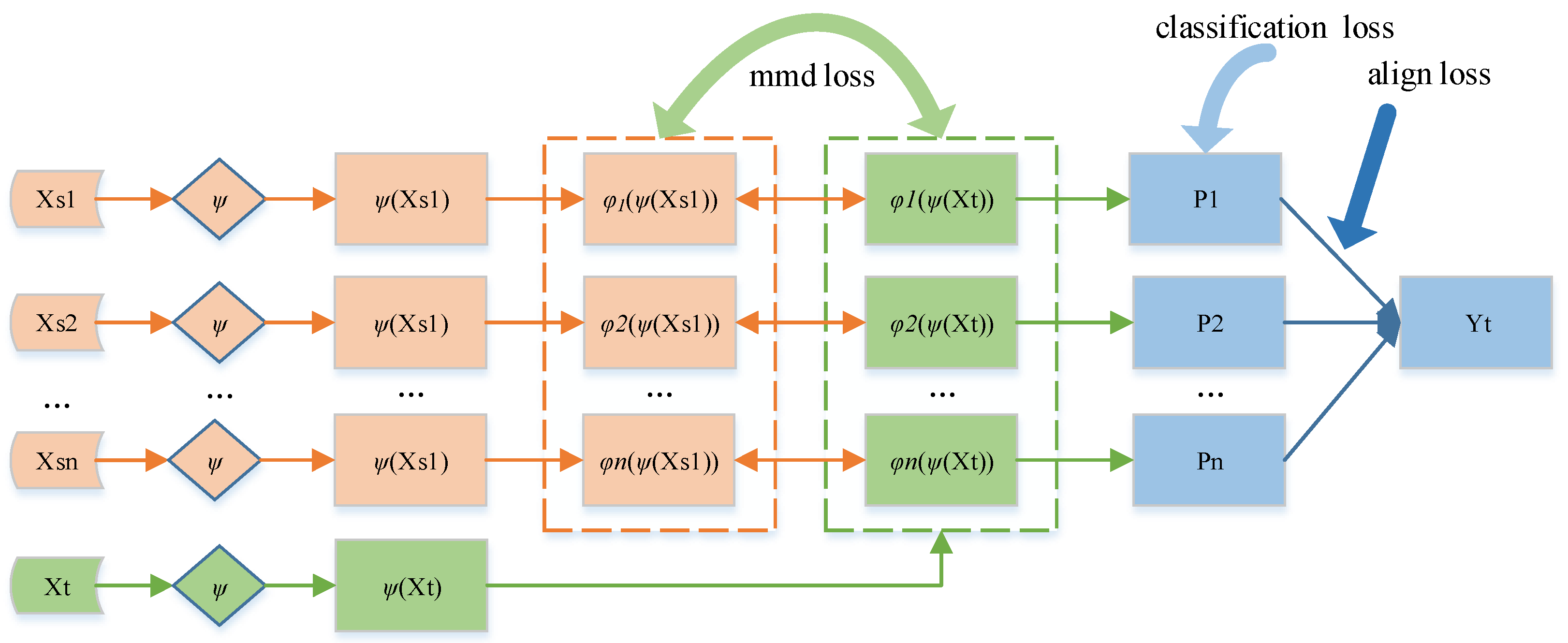
5.2. Method Framework and Implementation Details

The method framework of MSCPDP is shown in Figure 1. As the figure shows, MSCPDP first receives N source projects $X_{sj}$ and one target project $X_t$ as input. The symbol $\psi$ is a layer of network, which map the data of all projects from the original feature space to the common feature space. In order to use the data information of multiple source projects at the same time, we pair all input source projects and target project. Then, we construct N feature extractors ${\left\{{\phi }_j\right\}}_{j=1}^N$ and map each pair of source and target projects to a specific feature space. Moreover, we want to extract unique feature distribution for each pair of source and target projects. These N feature extractors work in parallel and do not share the same weight.

In order to map each pair of source project data and target project data to a specific feature space, we need to compare the data distribution of $\{{\phi }_j(\psi (x_{}^{sj}))\}$ and $\{{\phi }_j(\psi (x_{}^t))\}$. In the field of domain adaptation, several methods have been proposed to achieve this, such as adversarial loss [49], coral loss [50] and mmd loss [51]. In our method, choosing mmd loss as the loss function to reduce the difference in data distribution between the source project and the target project.

The Maximum Mean Discrepancy (MMD) is a kernel two-sample test which rejects or accepts the null hypothesis p = q based on the observed samples. The basic idea behind MMD is that if the generating distributions are identical, all the statistics are the same. MMD defines the following formal difference measures:

$$D_H(p,q)\triangleq \left|\right|E_p[\mathsf{\Phi }(x^s)]-E_q[\mathsf{\Phi }(x^t)]|{|}_H^2$$

(2)

where H is the reproducing kernel Hillbert space (RKHS) endowed with a characteristic kernel k. Here, $\mathsf{\Phi }$ denotes some feature map to map the original samples to RKHS and the kernel k means $k(x^{\mathrm{s}},x^t)=\langle \mathsf{\Phi }(x^s),\mathsf{\Phi }(x^t)\rangle$, where $\langle \rangle$ represents inner product of vectors. The main theoretical result is that p = q if and only if $D_H(p,q)=0$. In practice, an estimate of the MMD compares the square distance between the empirical kernel mean embeddings as:

$${\widehat{D}}_H(p,q)={\Vert \frac{1}{n_s}{\displaystyle \sum _{x_i\in D_S}\mathsf{\Phi }(x_i)}-\frac{1}{n_t}{\displaystyle \sum _{x_j\in D_T}\mathsf{\Phi }(x_j)}\Vert }_H^2$$

(3)

where ${\widehat{D}}_H(p,q)$ is an unbiased estimator of $D_H(p,q)$. Using (3) as the estimate of the discrepancy between each source domain and target domain, then, the mmd loss in our experiment is reformulated as:

$${\mathsf{\Gamma }}_{mmd}=\frac{1}{N}{\displaystyle \sum _{j=1}^N\stackrel{}{\widehat{D}}}({\phi }_j(\psi (X_{sj})),{\phi }_j(\psi (X_t)))$$

(4)

Next, building a softmax predictor for each pair of source and target projects, denoted by the symbol P. In this way, we have established a total of N predictors. For each predictor, using cross entropy to add classification loss:

$${\mathsf{\Gamma }}_{cls}={\displaystyle \sum _{j=1}^N{E}_{x\sim X_{sj}}}J(P_j({\phi }_j(\psi (x_i^{sj}))),y_i^{sj})$$

(5)

Finally, for each target project instance, we may generate a set of corresponding prediction results. These predictors are trained on different source projects, thus they may have different predictions on target instances, especially target instances near the classification boundary. Voting is a simple solution, but it sometimes performs poorly. Intuitively, the same target instance predicted by different classifiers should get the same prediction result. Therefore, using an alignment operation to minimize the difference between the predictions of all the predictors. We utilize the absolute values of the difference between all pairs of classifiers’ probabilistic outputs of target project data as alignment loss:

$${\mathsf{\Gamma }}_{als}=\frac{2}{N\ast (N-1)}{\displaystyle \sum _{j=1}^{N-1}{\displaystyle \sum _{i=j+1}^N{E}_{x~X_t}}\left[\left|P_i({\phi }_i(\psi (x_k^{})))-P_j({\phi }_j(\psi (x_k^{})))\right|\right]}$$

(6)

By minimizing (6), the probability outputs of all classifiers are similar. Thus, we can calculate the average of the output of all the predictors as the label of the target instance.

In general, the loss of our method includes three parts: classification loss, mmd loss and alignment loss. Specifically, by minimizing the mmd loss, the model maps each pair of source and target projects to a specific feature space; by minimizing the classification loss, the model can accurately classify the source project data; by minimizing the alignment loss, the model can reduce the output difference between the classifiers, so that the prediction becomes more accurate. The total loss formula is as (7):

$${\mathsf{\Gamma }}_{total}={\mathsf{\Gamma }}_{cls}+\lambda {\mathsf{\Gamma }}_{mmd}+\gamma {\mathsf{\Gamma }}_{als}$$

(7)

5.3. Experimental Parameter Setting

The paper used mini-batch stochastic gradient descent (SGD) with a momentum of 0.9. The batch size is set as 64. Following [52], using the learning rate annealing strategy: the learning rate is not selected by a grid search to high computation cost, it is adjusted during SGD using the following formula: ${\eta }_p=\frac{{\eta }_0}{{(1+\alpha p)}^{\beta }}$,where p is the training progress linearly changing from 0 to 1, ${\eta }_0=0.001$, α = 10 and β = 0.75, which is optimized to promote convergence and low error on the source project. To suppress noisy activations at the early stages of training, instead of fixing the adaptation factor λ and γ, we gradually change them from 0 to 1 by a progressive schedule: ${\gamma }_p={\lambda }_p=\frac{2}{\exp (-\theta p)}-1$, and θ = 10 is fixed throughout the experiments. The main code can be available at https://github.com/ZhaoYu-Lab/MSCPDP (accessed on 16 February 2022).

6. Experimental Research

This section introduces our experimental research. The previous experimental results tell us that single-source CPDP has two shortcomings, one is the poor performance lower limit, the other is the need to select the appropriate source project in order to get the optimal performance. Moreover, in most cases, the performance of multi-source merged is not even as good as the average value of single-source CPDP. As mentioned above, our method uses data information from multiple source projects at the same time, and its purpose is to solve the two shortcomings of single-source CPDP. Therefore, we still conducted experiments on the previously mentioned datasets, AEEEM and PROMISE, and compared them with the average performance of the current more advanced CPDP method. We still focused on observing the two index values of F1 and AUC.

6.1. Experimental Parameter Setting

In order to explore the performance of our MSCPDP method, we compared our method with the current more advanced methods. We combined the MSCPDP method with CamargoCruz [53], TCA+ [25], CKSDL [31], CTKCCA [32], HYDRA [30] and ManualDown [44]. These methods are the ones with good performance. The CamargoCruz method was evaluated by Herbold [54], and it was found that the classic CamargoCruz method always achieve the best performance.

TCA + and CTKCCA are effective transfer methods based on feature transformation. CKSDL is an effective semi-supervised CPDP method. HYDRA is an ensemble learning method using much labeled data from source project and a limited amount of labeled data from target project. ManualDown is an unsupervised method with excellent performance.

We set the following settings for the comparison method: for a given dataset, using one project of the dataset as the target project in turn, and use the other projects of the dataset as the source projects for cross-project prediction. For example, if the project EQ in the AEEEM dataset is selected as the target project, then the remaining projects (JDT, LC, ML, and PDE) in the AEEEM dataset are set as training projects once, and get four sets of EQ prediction results, namely JDT→EQ, LC→EQ, ML→EQ and PDE→EQ. On this basis, the average predicted value of the four sets of predicted results with EQ as the target project is calculated. As a result, we obtained the average F1 and AUC value of 15 target projects marked with the target project name. The experimental results are shown in

Table 4. Comparison of F1 value between MSCPDP and current advanced methods; bold is the maximum, * is the minimum.

Project	CamargoCruz	CKSDL	TCA+	CTKCCA	HYDRA	ManualDown	MSCPDP
EQ	0.6592	0.2709 *	0.4112	0.3530	0.5926	0.6742	0.3185
JDT	0.4732	0.3522	0.4093	0.3495 *	0.5385	0.3976	0.4218
LC	0.2448	0.3467	0.3631	0.3326	0.3774	0.2046 *	0.4355
ML	0.3238	0.3642	0.3581	0.3530	0.5385	0.2581 *	0.3246
PDE	0.3249	0.3507	0.4209	0.3495	0.2000 *	0.3009	0.3593
ant	0.4582	0.3497	0.4390	0.3177 *	0.3774	0.4853	0.5688
camel	0.3420	0.4614	0.3986	0.2404	0.1734 *	0.3333	0.3133
ivy	0.3477	0.3037 *	0.4510	0.2961	0.4400	0.3188	0.4717
jedit	0.3992	0.3028	0.1444 *	0.3588	0.4203	0.2843	0.5581
lucene	0.4022	0.2953 *	0.4441	0.3749	0.3273	0.6454	0.3213
poi	0.3713	0.2895	0.4117	0.4040	0.3333	0.5729	0.2866 *
synapse	0.4056	0.2583 *	0.3669	0.4099	0.5000	0.4933	0.5571
velocity	0.4635	0.2696 *	0.4598	0.4156	0.3447	0.5609	0.4132
xalan	0.5186	0.2652 *	0.4261	0.3967	0.3723	0.6225	0.4369
xerces	0.3000	0.3378	0.4033	0.3839	0.3200	0.2279 *	0.3803
mean	0.4028	0.3212 *	0.3938	0.3557	0.3904	0.4253	0.4113
median	0.3992	0.3976	0.3037 *	0.4112	0.3530	0.3774	0.4132

and

Table 5. Comparison of AUC value between MSCPDP and current advanced methods; boldface is the maximum, * is the minimum.

Project	CamargoCruz	CKSDL	TCA+	CTKCCA	HYDRA	ManualDown	MSCPDP
EQ	0.7406	0.5567 *	0.6572	0.6437	0.7666	0.7137	0.5750
JDT	0.7359	0.6028 *	0.5606	0.6430	0.7394	0.6212	0.6295
LC	0.7159	0.5660 *	0.6631	0.6456	0.7337	0.5902	0.6790
ML	0.7065	0.5940	0.6164	0.6437	0.7394	0.5690 *	0.6041
PDE	0.6964	0.5787 *	0.6628	0.6430	0.6532	0.6343	0.6411
ant	0.6732	0.5644 *	0.6442	0.5842	0.7331	0.6947	0.7287
camel	0.5743	0.5771	0.5794	0.5595 *	0.6838	0.5611	0.5683
ivy	0.6797	0.5969	0.7088	0.5516 *	0.7797	0.7119	0.7497
jedit	0.6198	0.6152	0.6439	0.6484	0.6763	0.4613 *	0.6959
lucene	0.6284	0.5855	0.5911	0.6647	0.5746 *	0.5980	0.5802
poi	0.6154	0.5371 *	0.6235	0.6867	0.6935	0.6611	0.5579
synapse	0.6518	0.5556 *	0.6211	0.6602	0.6762	0.5823	0.6826
velocity	0.5990 *	0.6093	0.6010	0.6569	0.6550	0.6395	0.6042
xalan	0.5884	0.5707 *	0.6821	0.6578	0.6743	0.5988	0.5918
xerces	0.6092	0.5838	0.6207	0.6392	0.6290	0.4873 *	0.6404
mean	0.6556	0.5796 *	0.6317	0.6352	0.6939	0.6083	0.6352
median	0.6518	0.5787 *	0.6235	0.6437	0.6838	0.5988	0.6295

.

6.2. Analysis of Experimental Results

Comparing the MSCPDP method with the current more advanced methods. We hope that our method can be similar to the average performance of these advanced methods, so that our method can achieve relatively good performance while avoiding the lower limit of performance, and ultimately has practical application value.

Table 4 and Table 5 have 8 columns and 18 rows, respectively. The first column in the table indicates the target project, and the second to seventh columns indicate the F1 and AUC value obtained by using the current advanced CPDP methods. The eighth column indicates the F1 and AUC value obtained by using our MSCPDP method to predict the target project. The second last row and the last row in the tables are the average value and median value of each column. Analyze the data in the second row of the Table 4 as an example. The second row uses EQ as the target project. The methods from the second column to the seventh column, CamargoCruz, CKSDL, TCA+, CTKCCA, HYDRA and ManualDown, all use EQ as the target project and perform JDT→EQ, LC→EQ, ML→EQ and PDE→EQ four groups of experiments, and then average the obtained F1 values to obtain 0.6592, 0.2709, 0.4112, 0.3530, 0.5926, and 0.6742, respectively. Our method MSCPDP in the last column uses JDT, LC, ML, and PDE data at the same time to construct a defect prediction model and then predict EQ to obtain an F1 value of 0.3185. Table 5 is the same analysis process as such.

First of all, from the point of view of F1 value, CKSDL has the minimum value in 6 out of 15 experiments, 3 times in ManualDown, 2 times each in HYDRA and CTKCCA, one time in TCA+, and our method MSCPDP has achieved the minimum F1 only once. In addition, about the maximum F1 value, CKSDL achieved the largest F1 value once, TCA+ and HYDRA each twice, ManualDown five times, and our method five times. Thus, in terms of quantity, our method MSCPDP does perform better since our method achieved a large number of maximums and a small number of minimums. From a detailed point of view, we are comparing the average F1 value of the previous methods. For example, with LC as the target project, our method MSCPDP achieved the best F1 value of 0.4355, while the F1 value obtained by CamargoCruz was 0.2448, which shows the average F1 value of the four sets of experiments performed using the CamargoCruz method is 0.2448, which can indicate that the performance of our MSCPDP method exceeds most of the four sets of experiments conducted by the CamargoCruz method, and may exceed two of them, and even the maximum value of the four sets of experiments conducted by the CamargoCruz method does not exceed 0.4355. Taking velocity as the target project again, although the best F1 value is 0.5609 of the ManualDown method, the F1 value of our MSCPDP method is 0.4132, which is close to the average F1 value of the ManualDown method, which shows that the average value of 9 sets of experiments conducted by the ManualDown method with velocity as the target project is 0.5609, and our F1 value of 0.4132 may exceed the F1 value of 3 out of 9 sets of experiments or 4 sets of experiments, although not necessarily the best F1 in 9 sets of experiments value, but also exceeded the F1 value of most experiments in the 9 groups.

From the AUC value, the results are similar. MSCPDP does not have a minimum value, but has three maximum values. In addition, from the average and median of the two indicators, ManualDown achieved the largest overall average of F1 indicators, MSCPDP was the second largest, but MSCPDP achieved the largest overall median. Moreover, MSCPDP achieved the third-largest overall average value of AUC indicators, and the overall median value we are in the fourth place. These fully shows that our method can reach the average or above level with the current advanced methods. However, we can find that the performance of HYDRA is very good; in fact, it is true, because HYDRA uses an ensemble learning method and some marked target project instances, but HYDRA also has the drawbacks that we mentioned earlier. This means that the average performance on camel is only 0.1734, which means that they get the worst performance here. Thus, it is necessary to use multi-source at the same time for defect prediction in practice.

Therefore, from this perspective, we can find that we can indeed acquire knowledge related to the target project from multiple source projects at the same time, and the defect prediction model constructed can avoid the worst performance even if the best performance cannot be achieved in practice. Relatively speaking, our MSCPDP method can improve the performance of cross-project defect prediction and reach the average or above level of the current advanced methods. This is very important in practice, because we cannot know in advance which source project to build the model will get the best performance, so we can avoid the two shortcomings of current advanced CPDP methods, one is the poor performance lower limit, the other is the need to select the appropriate source project in order to get the optimal performance, and we also reach or exceed its average performance, which is very valuable.

6.3. Discussion

First of all, it needs to be clear whether the experimental exploration of single source CPDP and multi-source CPDP is meaningful. The answer is yes. For most current CPDP studies, single source CPDP only uses the data information of a single source project. In multi-source CPDP studies, one part uses heuristic methods to select similar source projects, and the other part simply combines the data volume of multiple source projects. The experimental results of this paper show that the setting of single source CPDP cannot know the best source project in advance in practice, while the setting of multi-source CPDP is often not so effective when using heuristic search method for the best source project, and the selected source project sometimes has the problem of lower performance limit; When merging multiple source projects to expand the amount of data, multiple data distributions are not considered. These problems are real in practice, thus they have practical significance.

Secondly, for the two problems found in the experiment, whether the MSCPDP method proposed in this paper has practical value, the answer is also yes. The method proposed in this paper considers the data distribution of multiple source projects at the same time. It not only uses the data information of multiple source projects, but also pays attention to the data differences between multiple source projects and target projects. At the same time, this method also successfully avoids the selection of single source CPDP in source projects in practice. From the experimental results, the proposed method has practical significance.

Finally, it needs to be clear whether our method has some limitations. It is certain that any method will have some limitations. For the method proposed in this paper, with the growth of the number of open source projects, it must be desirable. This paper uses all available source projects in the experiment, but a natural question is: how does one choose if the number of source projects is too large? The increase in number will lead to more redundancy and greater data differences. From this point of view, the method proposed in this paper also needs to carry out element control analysis on a larger dataset.

7. Conclusions and Future Work

Although the current experimental performance of cross-project defect prediction is not bad, in practice, it is difficult to determine which source project to use to train the defect prediction model to get the best performance and if the source project data used to build the model is inappropriate, it will lead to extremely poor performance. Aiming at this problem, this paper proposes a new solution, i.e., simultaneously using the knowledge of multiple source projects related to the target project to construct a defect prediction model. This paper first explores the practical significance and existing problems of the cross-project defect prediction method based on multiple sources, and then according to the existing problems, we propose a multi-source-based cross-project defect prediction method MSCPDP, which can solve the problem of data distribution differences between multiple source projects and target projects when the data of multiple source projects are used at the same time. Experiments show that, compared with the current more advanced CPDP methods, MSCPDP can achieve comparable performance on F1 and AUC and can effectively avoid the two shortcomings of the current cross-project defect prediction method based on a single source project.

However, there are still many subsequent steps worth discussing in this paper. First of all, we found that our MSCPDP method cannot completely defeat the current more advanced methods. We hope that our multi-source and cross-project defect method should be able to defeat the best performance of a single-source single-target setting, instead of just avoiding the worst performance and at the same level with them. We believe that the feature distortion phenomenon in the original feature space leads to unsatisfactory results in reducing the difference in data distribution between each pair of source projects and target projects, which leads to poor results in some experiments. Secondly, our MSCPDP chooses the simplest network and classifier. Later, a better performance model can be selected for research to see if the performance of multi-source and cross-project defect prediction can be improved, such as integrating different types of models. Finally, when all source project data are available, we use all source projects. One question is that using more source projects and different source projects will introduce more redundant data and greater data distribution differences; therefore, how to reduce redundant data and data distribution differences and how to maintain the balance of quantity combination and performance when using multiple source projects is the next step worth studying.

References

- Gotlieb, A. Exploiting symmetries to test programs. In Proceedings of the 14th International Symposium on Software Reliability Engineering, Denver, CO, USA, 17–21 November 2003. [Google Scholar]
- Gomez-Jauregui, V.; Hogg, H.; Manchado, C. GomJau-Hogg’s Notation for automatic generation of k-uniform tessellations with ANTWERP v3.0. Symmetry 2021, 13, 2376. [Google Scholar] [CrossRef]
- Chen, X.; Gu, Q.; Liu, W.; Ni, C. Survey of static software defect prediction. J. Softw. 2016, 27, 1–25. [Google Scholar]
- Jin, C. Software defect prediction model based on distance metric learning. Soft Comput. 2021, 25, 447–461. [Google Scholar] [CrossRef]
- Hall, T.; Beecham, S.; Bowes, D.; Gray, D.; Counsell, S. A systematic literature review on fault prediction performance in software engineering. IEEE Trans. Softw. Eng. 2012, 38, 1276–1304. [Google Scholar] [CrossRef]
- Chen, X.; Mu, Y.; Liu, K.; Cui, Z.; Ni, C. Revisiting heterogeneous defect prediction methods: How far are we? Inf. Softw. Technol. 2021, 130, 106441. [Google Scholar] [CrossRef]
- Hosseini, S.; Turhan, B.; Mika, M. A benchmark study on the effectiveness of search-based data selection and feature selection for cross project defect prediction. Inf. Softw. Technol. 2018, 95, 296–312. [Google Scholar] [CrossRef] [Green Version]
- Chen, X.; Wang, L.; Gu, Q.; Wang, Z.; Ni, C.; Liu, W.; Wang, Q. A survy on cross-project software defect prediction methods. Chin. J. Comput. 2018, 41, 254–274. [Google Scholar]
- Gong, L.; Jiang, S.; Jiang, L. Research progress of software defect prediction. J. Softw. 2019, 30, 3090–3114. [Google Scholar]
- Hosseini, S.; Turhan, B.; Gunarathna, D. A systematic literature review and meta-analysis on cross project defect prediction. IEEE Trans. Softw. Eng. 2019, 45, 111–147. [Google Scholar] [CrossRef] [Green Version]
- Wang, X.; Xia, X.; Hassan, A.; David, L.; Yin, J.; Yang, X. Perceptions, expectations, and challenges in defect prediction. IEEE Trans. Softw. Eng. 2020, 46, 1241–1266. [Google Scholar]
- Li, Y.; Liu, Z.; Zhang, H. Review on cross-project software defects prediction methods. Comput. Technol. Dev. 2020, 30, 98–103. [Google Scholar]
- Pan, S.J.; Tsang, I.W.; Kwok, J.T.; Yang, Q. Domain adaptation via transfer component analysis. IEEE Trans. Neural Netw. 2010, 22, 199–210. [Google Scholar] [CrossRef] [Green Version]
- Cheng, M.; Wu, G.Q.; Yuan, M.T. Transfer Learning for Software Defect Prediction. Acta Electron. Sin. 2016, 44, 115–122. [Google Scholar]
- He, Z.; Shu, F.; Yang, Y.; Li, M.; Wang, Q. An investigation on the feasibility of cross-project defect prediction. Autom. Softw. Eng. 2012, 19, 167–199. [Google Scholar] [CrossRef]
- Herbold, S. Training data selection for cross-project defect prediction. In Proceedings of the 9th International Conference on Predictive Models in Software Engineering, New York, NY, USA, 1–10 October 2013. [Google Scholar]
- Turhan, B.; Menzies, T.; Bener, A.B.; Stefano, J.D. On the relative value of cross-company and within-company data for defect prediction. Empir. Softw. Eng. 2009, 14, 540–578. [Google Scholar] [CrossRef] [Green Version]
- Peters, F.; Menzies, T.; Marcus, A. Better cross company defect prediction. In Proceedings of the 2013 10th Working Conference on Mining Software Repositories (MSR), San Francisco, CA, USA, 18–19 May 2013; pp. 409–418. [Google Scholar]
- He, P.; Li, B.; Zhang, D.; Ma, Y. Simplification of training data for cross-project defect prediction. arXiv 2014, arXiv:1405.0773. [Google Scholar]
- Li, Y.; Huang, Z.; Wang, Y.; Huang, B. New approach of cross-project defect prediction based on multi-source data. J. Jilin Univ. 2016, 46, 2034–2041. [Google Scholar]
- Asano, T.; Tsunoda, M.; Toda, K.; Tahir, A.; Bennin, K.E.; Nakasai, K.; Monden, A.; Matsumoto, K. Using Bandit Algorithms for Project Selection in Cross-Project Defect Prediction. In Proceedings of the 2021 IEEE International Conference on Software Maintenance and Evolution (ICSME), Luxembourg, 27 September–1 October 2021; pp. 649–653. [Google Scholar]
- Wu, J.; Wu, Y.; Niu, N.; Zhou, M. MHCPDP: Multi-source heterogeneous cross-project defect prediction via multi-source transfer learning and autoencoder. Softw. Qual. J. 2021, 29, 405–430. [Google Scholar] [CrossRef]
- Briand, L.C.; Melo, W.L.; Wust, J. Assessing the applicability of fault-proneness models across object-oriented software projects. IEEE Trans. Softw. Eng. 2002, 28, 706–720. [Google Scholar] [CrossRef] [Green Version]
- Zimmermann, T.; Nagappan, N.; Gall, H.; Giger, E.; Murphy, B. Cross-project defect prediction: A large scale experiment on data vs. domain vs. process. In Proceedings of the 7th Joint Meeting of the European Software Engineering Conference and the ACM SIGSOFT Symposium on The Foundations of Software Engineering, Amsterdam, The Netherlands, 24–28 August 2009; pp. 91–100. [Google Scholar]
- Nam, J.; Pan, S.J.; Kim, S. Transfer defect learning. In Proceedings of the 2013 35th International Conference on Software Engineering (ICSE), San Francisco, CA, USA, 18–26 May 2013; pp. 382–391. [Google Scholar]
- Ma, Y.; Luo, G.; Zeng, X.; Chen, A. Transfer learning for cross-company software defect prediction. Inf. Softw. Technol. 2012, 54, 248–256. [Google Scholar] [CrossRef]
- Yu, Q.; Jiang, S.; Zhang, Y. A feature matching and transfer approach for cross-company defect prediction. J. Syst. Softw. 2017, 132, 366–378. [Google Scholar] [CrossRef]
- Yu, Q.; Jiang, S.; Qian, J. Which is more important for cross-project defect prediction: Instance or feature? In Proceedings of the 2016 International Conference on Software Analysis, Testing and Evolution (SATE), Kunming, China, 3–4 November 2016; pp. 90–95. [Google Scholar]
- Yu, Q.; Qian, J.; Jiang, S.; Wu, Z.; Zhang, G. An empirical study on the effectiveness of feature selection for cross-project defect prediction. IEEE Access 2019, 7, 35710–35718. [Google Scholar] [CrossRef]
- Xia, X.; Lo, D.; Pan, S.J.; Nagappan, N.; Wang, X. Hydra: Massively compositional model for cross-project defect prediction. IEEE Trans. Softw. Eng. 2016, 42, 977–998. [Google Scholar] [CrossRef]
- Wu, F.; Jing, X.Y.; Sun, Y.; Sun, J.; Huang, L.; Cui, F.; Sun, Y. Cross-project and within-project semi supervised software defect prediction: A unified approach. IEEE Trans. Reliab. 2018, 67, 581–597. [Google Scholar] [CrossRef]
- Li, Z.; Jing, X.Y.; Wu, F.; Zhu, X.; Xu, B.; Ying, S. Cost-sensitive transfer kernel canonical correlation analysis for heterogeneous defect prediction. Autom. Softw. Eng. 2018, 25, 201–245. [Google Scholar] [CrossRef]
- Zhang, Y.; Lo, D.; Xia, X.; Sun, J. An empirical study of classifier combination for cross-project defect prediction. In Proceedings of the 2015 IEEE Computer Software & Applications Conference, Taichung, Taiwan, 1–5 July 2015; pp. 264–269. [Google Scholar]
- Chen, J.; Hu, K.; Yang, Y.; Liu, Y.; Xuan, Q. Collective transfer learning for defect prediction. Neurocomputing 2020, 416, 103–116. [Google Scholar] [CrossRef]
- Yu, X.; Wu, M.; Jian, Y.; Bennin, K.E.; Fu, M.; Ma, C. Cross-company defect prediction via semi-supervised clustering-based data filtering and MSTrA-based transfer learning. Soft Comput. 2018, 22, 3461–3472. [Google Scholar] [CrossRef]
- Lelis, L.; Sander, J. Semi-supervised density-based clustering. In Proceedings of the 2009 9th IEEE International Conference on Data Mining, Miami Beach, FL, USA, 6–9 December 2009; pp. 842–847. [Google Scholar]
- Peng, L.; Yang, B.; Chen, Y.; Abraham, A. Data gravitation based classification. Inf. Sci. 2009, 179, 809–819. [Google Scholar] [CrossRef]
- Yao, Y.; Doretto, G. Boosting for transfer learning with multiple sources. In Proceedings of the 2010 IEEE Computer Society Conference on Computer Vision and Pattern Recognition, San Francisco, CA, USA, 13–18 June 2010; pp. 1855–1862. [Google Scholar]
- Sun, Z.; Li, J.; Sun, H.; He, L. CFPS: Collaborative filtering based source projects selection for cross-project defect prediction. Appl. Soft Comput. 2021, 99, 106940. [Google Scholar] [CrossRef]
- Adomavicius, G.; Tuzhilin, A. Toward the next generation of recommender systems: A survey of the state-of-the-art and possible extensions. IEEE Trans. Knowl. Data Eng. 2005, 17, 734–749. [Google Scholar] [CrossRef]
- D’Ambros, M.; Lanza, M.; Robbes, R. Evaluating defect prediction approaches: A benchmark and an extensive comparison. Empir. Softw. Eng. 2012, 17, 531–577. [Google Scholar] [CrossRef]
- Jureczko, M.; Madeyski, L. Towards identifying software project clusters with regard to defect prediction. In Proceedings of the 6th International Conference on Predictive Models in Software Engineering, Timisoara, Romania, 12–13 September 2010; pp. 1–10. [Google Scholar]
- Chidamber, S.R.; Kemerer, C.F. A metrics suite for object oriented design. IEEE Trans. Softw. Eng. 1994, 20, 476–493. [Google Scholar] [CrossRef] [Green Version]
- Zhou, Y.; Yang, Y.; Lu, H.; Chen, L.; Li, Y.; Zhao, Y.; Qian, J.; Xu, B. How far we have progressed in the journey? An examination of cross-project defect prediction. ACM Trans. Softw. Eng. Methodol. 2018, 27, 1–51. [Google Scholar] [CrossRef]
- Xu, R.; Chen, Z.; Zuo, W.; Yan, J.; Lin, L. Deep cocktail network: Multi-source unsupervised domain adaptation with category shift. In Proceedings of the IEEE Conference on Computer Vision and Pattern Recognition (CVPR), Salt Lake City, UT, USA, 18–23 June 2018; pp. 3964–3973. [Google Scholar]
- Zhao, H.; Zhang, S.; Wu, G.; Gordon, G.J. Multiple source domain adaptation with adversarial learning. In Proceedings of the 6th International Conference on Learning Representations (ICLR), Vancouver, BC, Canada, 16 February 2018. [Google Scholar]
- Zhu, Y.; Zhuang, F.; Wang, D. Aligning domain-specific distribution and classifier for cross-domain classification from multiple sources. In Proceedings of the AAAI Conference on Artificial Intelligence, Palo Alto, CA, USA, 17 July 2019; Volume 33, pp. 5989–5996. [Google Scholar]
- Zeng, J.; Xie, P. Contrastive self-supervised learning for graph classification. arXiv 2020, arXiv:2009.05923. [Google Scholar]
- Tzeng, E.; Hoffman, J.; Darrell, T.; Saenko, K. Simultaneous deep transfer across domains and tasks. In Proceedings of the IEEE International Conference on Computer Vision (ICCV), Santiago, Chile, 7–13 December 2015; pp. 4068–4076. [Google Scholar]
- Sun, B.; Saenko, K. Deep coral: Correlation alignment for deep domain adaptation. In Proceedings of the European Conference on Computer Vision (ECCV), Amsterdam, The Netherlands, 8–10 October 2016; pp. 443–450. [Google Scholar]
- Gretton, A.; Borgwardt, K.M.; Rasch, M.J.; Schölkopf, B.; Smola, A. A kernel two-sample test. J. Mach. Learn. Res. 2012, 13, 723–773. [Google Scholar]
- Ganin, Y.; Lempitsky, V. Unsupervised domain adaptation by backpropagation. In Proceedings of the 32nd International Conference on Machine Learning (PMLR), Lille, France, 7–9 July 2015; pp. 1180–1189. [Google Scholar]
- Cruz, A.E.C.; Ochimizu, K. Towards logistic regression models for predicting fault-prone code across software projects. In Proceedings of the 2009 3rd International Symposium on Empirical Software Engineering and Measurement, Lake Buena Vista, FL, USA, 15–16 October 2009; pp. 460–463. [Google Scholar]
- Herbold, S.; Trautsch, A.; Grabowski, J. A comparative study to benchmark cross-project defect prediction approaches. IEEE Trans. Softw. Eng. 2018, 44, 811–833. [Google Scholar] [CrossRef]
Publisher’s Note: MDPI stays neutral with regard to jurisdictional claims in published maps and institutional affiliations. |
© 2022 by the authors. Licensee MDPI, Basel, Switzerland. This article is an open access article distributed under the terms and conditions of the Creative Commons Attribution (CC BY) license (https://creativecommons.org/licenses/by/4.0/).