Condition Monitoring of Rolling Bearing Based on Multi-Order FRFT and SSA-DBN

Abstract

Owing to the symmetry of the rolling bearing structure and the rotating operation mode, the rolling bearing works in a complex environment. It is very easy to be submerged by noise and misdiagnosis. For the non-stationary signal in variable speed state, this paper presents a condition monitoring method based on deep belief network (DBN) optimized by multi-order fractional Fourier transform (FRFT) and sparrow search algorithm (SSA). Firstly, the fractional Fourier transform based on curve feature segmentation is used to filter the fault vibration signal and extract the fault feature frequency. Then, the fault features are input into the SSA-DBN model for training, and the bearing fault features are classified, identified, and diagnosed. Finally, the rotating machinery fault simulator in the laboratory of Ottawa University is taken as the practical application object to verify the effectiveness of the method. The experimental results show that the proposed method has higher recognition accuracy and stronger stability.

1. Introduction

As one of the key components of rotating machinery, rolling bearings are widely used in electric power, shipbuilding, chemical, nuclear power, and other engineering fields [1]. Owing to the symmetry of the rolling bearing structure and the rotating operation mode, they are often used under high temperature and high speed conditions. Once a fault occurs, it will cause economic losses and casualties [2]. Therefore, the condition monitoring of rolling bearings has very important theoretical significance and application value for ensuring its safe and reliable operation [3]. If the rolling bearing fault is not detected and dealt with early, the incipient fault will gradually develop into a more serious fault [4,5]. For example, in 1992, a Japanese power plant caused an overload accident due to a bearing fault, which not only lost billions of yen, but also caused casualties. In 2006, the bearing of a spinning machine in Anyang Iron and Steel Company was broken, which caused the whole plant’s production line to be interrupted and resulted in huge economic losses. In 2007, a train derailment accident occurred within the jurisdiction of Zhengzhou Railway Bureau. In 2007, a train derailment accident occurred within the jurisdiction of Zhengzhou Railway Bureau. Because the bearing failure was not found and dealt with in time at the initial stage, the train was derailed and distressed. In 2014, a Russian helicopter failed to detect and repair the early engine bearing failure, which eventually led to a crash of the aircraft and personnel were injured or killed. Therefore, the condition monitoring of rolling bearing has extremely important practical significance and engineering application value for ensuring the safe operation of equipment [6].

Condition monitoring is one of the hot research topics at home and abroad. If the incipient faults are not detected and dealt with in time, it will have a destructive impact on the safe operation of the system [7,8,9]. In 2012, Li and Zhou et al. [10] summarized the research status of weak fault diagnosis at home and abroad in literature. According to the characteristics of weak faults, the classification framework of weak fault diagnosis is proposed. The weak fault diagnosis methods are divided into three categories: qualitative diagnosis methods (graph theory method and expert system), quantitative diagnosis methods and semi-qualitative and semi-quantitative diagnosis methods [11,12]. In 2016, Wen et al. [13] classified “micro fault diagnosis methods based on data drive” into three categories: statistical analysis methods, signal processing methods and artificial intelligence methods.

In signal processing methods, fractional Fourier transform is one of the important directions of non-stationary signal processing, which was first widely used in radar, communication, information security, and other fields [14,15,16]. As a high-resolution and fine adaptive filtering method, FRFT makes use of the characteristics of different energy concentrations of non-stationary signals in the fractional order domain of different orders. So that the micro fault has the best energy aggregation in the fractional order domain, while other components and noise will not gather in the fractional order domain [17,18]. The weak fault feature information can be extracted by narrow-band masking in the fractional order domain. In recent years, [19] used FRFT for early fault diagnosis of gearbox; while [20] used FRFT to extract weak fault features of rolling bearings. However, in practical work, rolling bearings mostly operate at variable speed, and their fault characteristic frequency presents as a curvilinear nonlinear frequency modulation (NLFM).

NLFM is a typical time-varying non-stationary signal, and the same component will gather in multiple fractional order domains, so it is difficult to determine the optimal order of FRFT filtering according to the peak value. Thus, the early fault cannot be separated, and the single-order FRFT filter fails [21]. Aiming at the problem that it is difficult to extract the fault features of variable speed bearing under the interference of strong background noise, a piecewise multi-order FRFT filtering method based on curve features is proposed in this paper. The signal with NLFM is piecewise linearized and filtered in the fractional domain. This method can effectively filter the noise and accurately extract the characteristic frequency of early fault.

With its strong nonlinear ability, deep belief network has significant advantages in feature recognition, classification, and nonlinear mapping. At present, it has been widely used in the field of fault diagnosis [22]. The authors of [23] proposed an intelligent integration method based on the deep belief network (DBN), which can accurately and efficiently diagnose the fault of planetary gearbox of wind turbine; while [24] applied deep belief network to power system fault diagnosis, and enhanced the ability of feature extraction and fault classification by improving the network model; and [25] combined the deep belief network with fuzzy mean clustering algorithm to realize the fault diagnosis of rolling bearing without a sample label.

As DBN initializes model parameters randomly in practical applications, it is not conducive to the training of network parameters and will affect the classification accuracy of the network. As the sparrow search algorithm is a swarm intelligence optimization algorithm, it is not affected by the characteristics of the objective function, such as whether the function is differentiable, differentiable, continuous, and so on. It is an intelligent algorithm with good stability, high computing efficiency, and fast convergence speed. Therefore, the classification accuracy of the network can be effectively improved. Based on this, this paper uses the sparrow search algorithm to optimize the weight parameters of the DBN, so that it can adaptively determine the initial model parameters, which can effectively improve the classification accuracy and efficiency, and meet the needs of real-time diagnosis.

The rest of this paper is organized as follows. In Section 2, some basic theories are reviewed and details of the proposed method are presented. Section 3 shows a clearer bearing diagnosis process with experimental signals and demonstrates the robustness of the proposed method. The conclusions are summarized in Section 4.

2. Related Theories

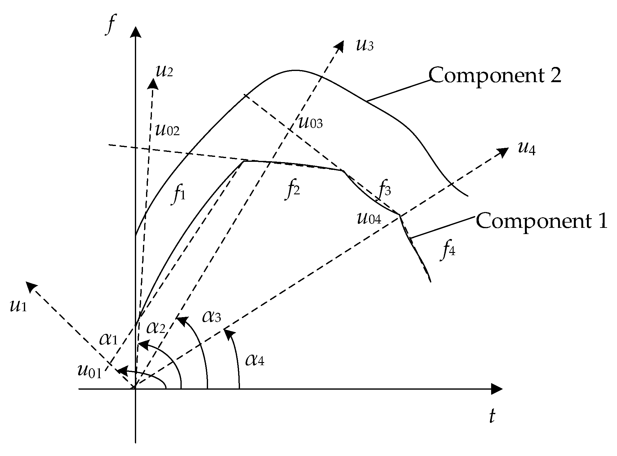
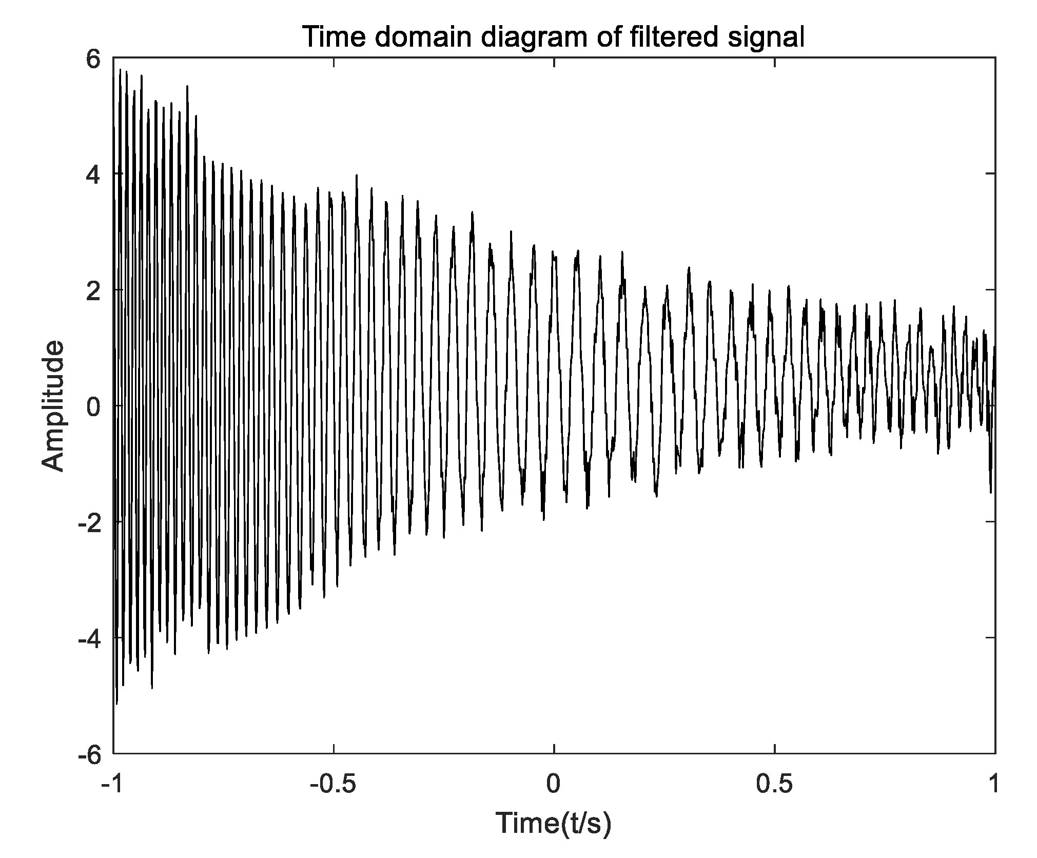
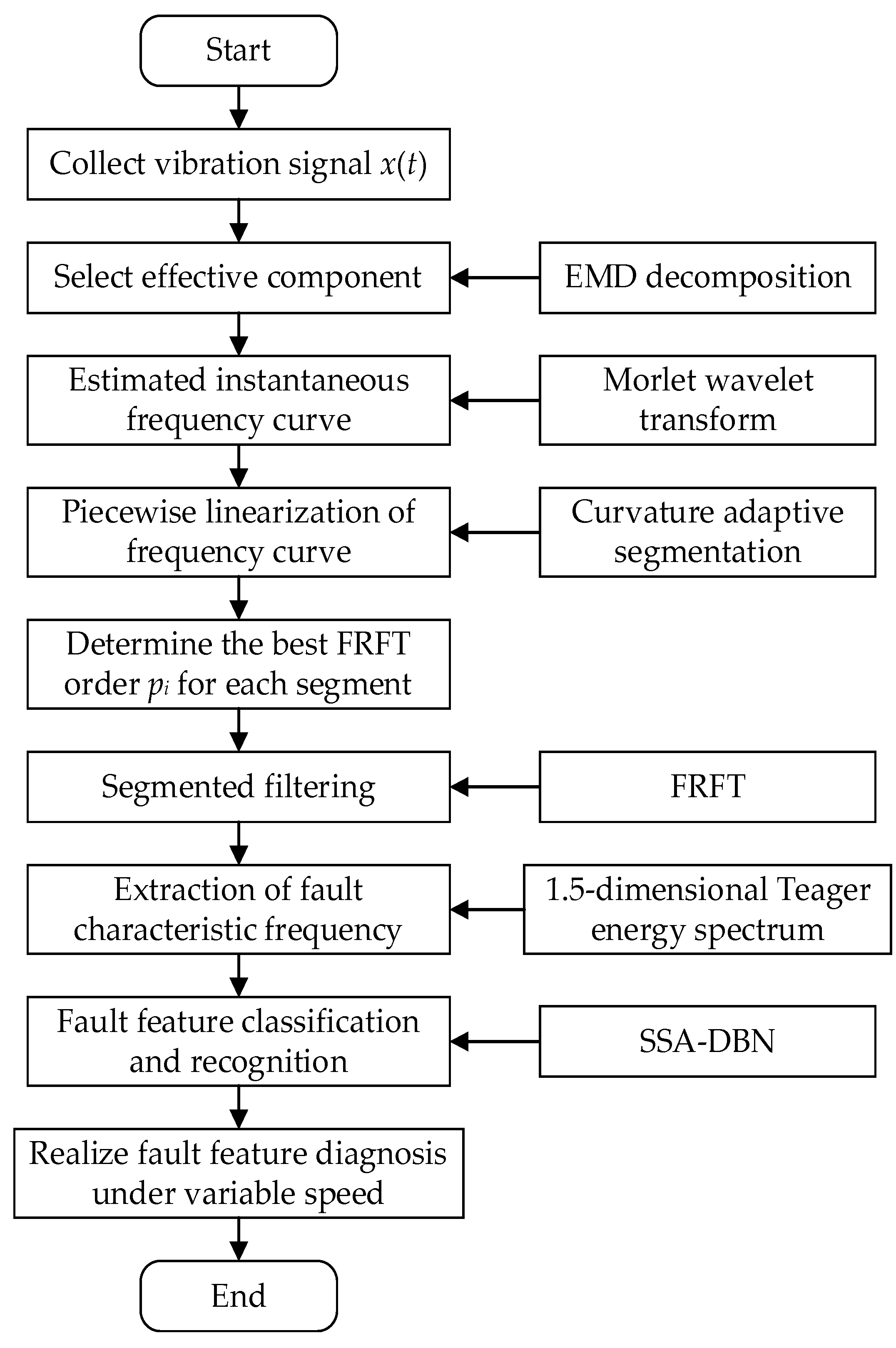
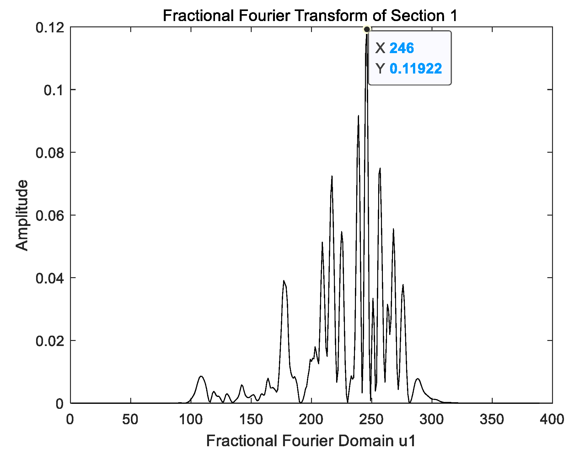
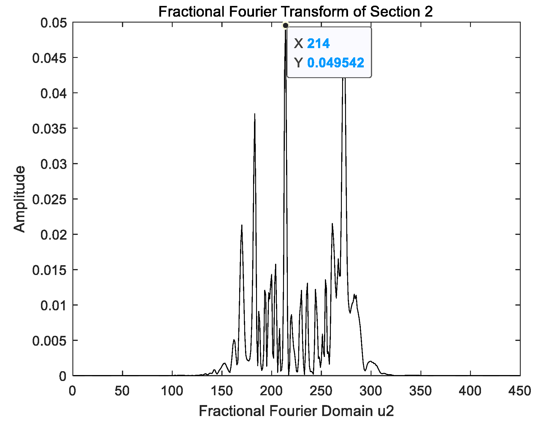
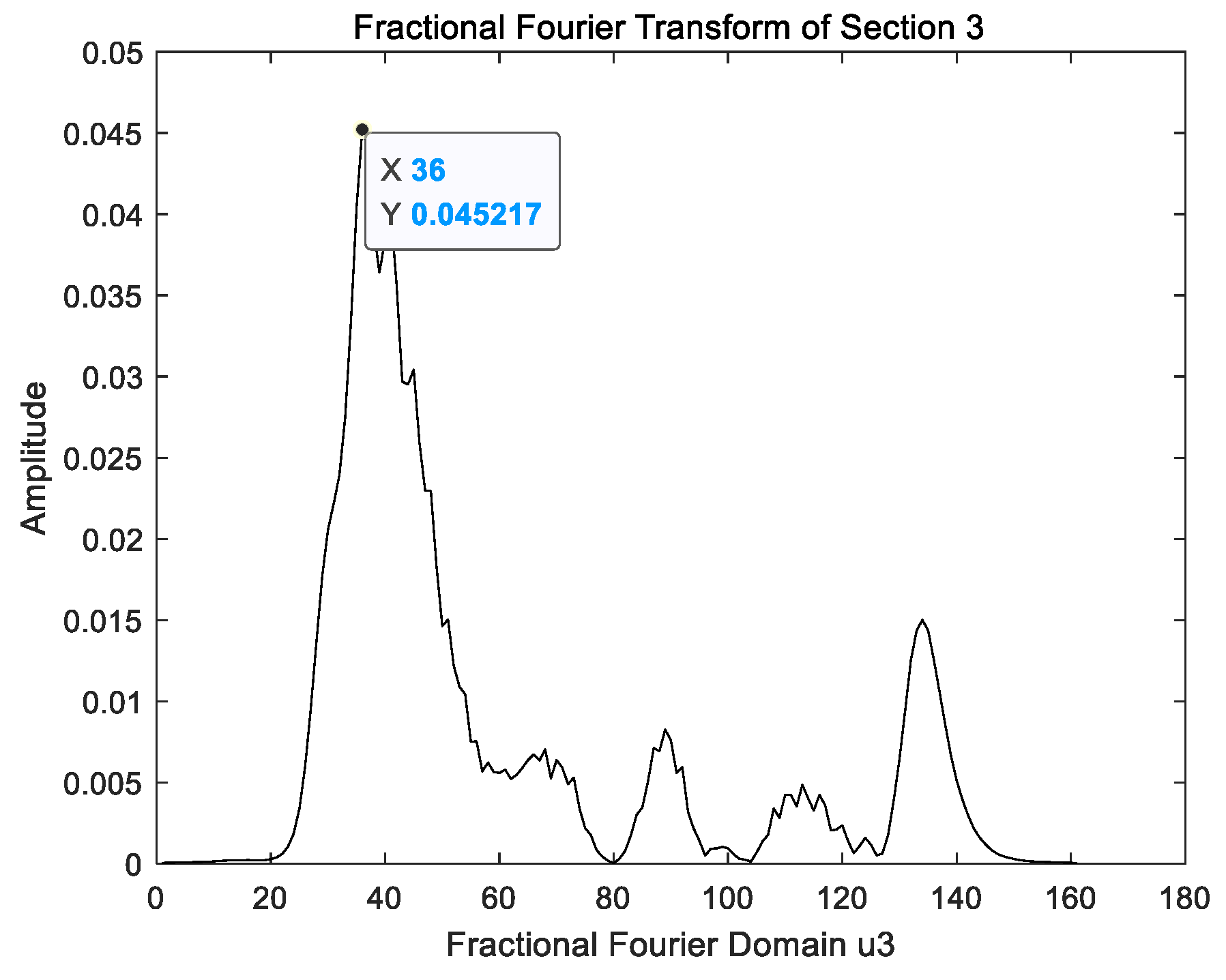
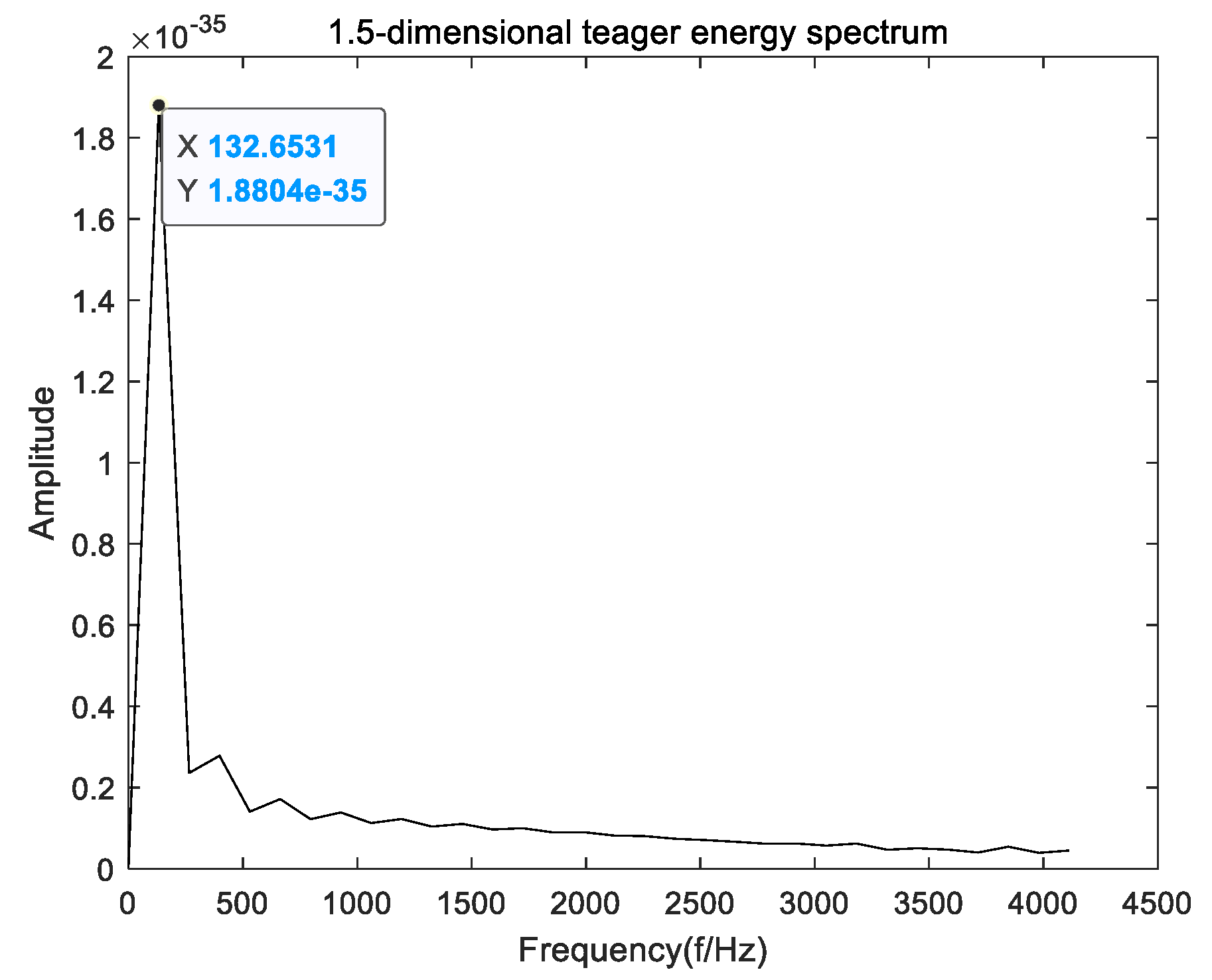
2.1. Signal Filtering Method Based on FRFT

The concept of fractional Fourier transform was firstly proposed by Wiener in 1929 [24]. FRFT is a method of transforming signals from time domain to fractional domain. It is a generalized form of Fourier transform. Its forward and inverse transform pairs are as follows:

$$\begin{gathered} X_p(u)=F_p[x](u)={\displaystyle {\int }_{-\infty }^{+\infty }x(t)K_p(t,u)dt}, \\ x(t)={\displaystyle {\int }_{-\infty }^{+\infty }{X}_p(u)K_{-p}(t,u)du}. \end{gathered}$$

(1)

where the kernel function Kp(t, u) of FRFT is as follows:

$$K_p(t,u)=\{\begin{array}{l}{A}_{\alpha }\exp (j\pi \frac{t^2+u^2}{2}{\cot }_{\alpha }-j\pi tu\csc c_{\alpha }),\begin{array}{c}\end{array}\alpha \ne n\pi \\ \delta (t-u),\begin{array}{c}\end{array}\alpha =2n\pi \\ \delta (t+u),\begin{array}{c}\end{array}\alpha =(2n\pm 1)\pi \end{array}$$

(2)

where α = pπ/2 denotes the rotation angle and p denotes order. When p = 1, FRFT becomes Fourier transform.

Set the time-frequency distribution of two linear frequency modulation (LFM) signals, as shown in Figure 1. Where the included angle between the time-frequency distribution of one LFM signal and the time axis is β. If the rotation angles α and β are orthogonal, the LFM signal should focus on u0 in the fractional order domain. Further, the energy of the noise is evenly distributed in the whole time domain plane, and there will be no energy aggregation in any fractional order domain. The feature extraction of LFM signal can be realized by taking the focus u0 of fractional order domain as the center for narrowband filtering and inverse FRFT transform.

It can be obtained from Figure 1 that the relationship during the best rotation angle α, order p, and modulation frequency f_m is as follows:

$$\begin{array}{l}\beta =\arctan (f_m),\\ \alpha =\frac{\pi }{2}+\beta =\frac{\pi }{2}+\arctan (f_m),\\ p=\alpha \frac{\pi }{2}=1+\frac{2}{\pi }\arctan (f_m).\end{array}$$

(3)

Set the time-frequency distribution of two nonlinear frequency modulation (NLFM) signals, as shown in Figure 2. The frequency of both signals changes in a curve, and in the single-order FRFT filter rotating, only one angle fails. Multi-order FRFT filtering is centered on u₀₁, u₀₂, …, u₀₄ in multiple fractional order domains u₁, u₂, …, u₄ by rotating multiple angles a₁, a₂, …, a₄ in turn. In theory, NLFM signal can be separated and then filtered by single-order FRFT.

The signal whose frequency changes in a curve is adaptively divided into several signal segments whose frequency changes approximately linearly, as shown in Figure 3. Then, the optimal filtering order of each segment of signal FRFT is determined according to the modulation frequency f_m of each signal segment, and it is filtered segment by segment.

The specific steps are as follows:

Step 1: Normalize the frequency curve of the original vibration signal and segment it, so that each frequency curve is approximately linear. According to the curvature formula $\mathrm{K}=\left|{\mathrm{y}}^{″}/{{(1+\mathrm{y}}^{\prime })}^{\frac{3}{2}}\right|$, calculate the curvature of points on the curve with a preset step size, and calculate the curvature difference K_i between two points in unit interval step. The curvature difference between both points is accumulated. If the sum meets the preset conditions, all points corresponding to curvature difference are divided into a segment interval in turn, and the frequency curve is divided into several segments; that is, set a threshold K_e. Accumulate from the first curvature difference. If K₁ + K₂ + … + K_m ≥ K_e, 1 ~ m + 1 points are divided into a segmented interval, and then restart accumulation from K_m+1 until the next segment interval is obtained, and divide the curve into several segments in turn. Each segment can be approximated to a straight line by adjusting the threshold. Component 1 can be adaptively divided into four segments (i.e., f₁, f₂, f₃, and f₄), as shown in Figure 3.

Step 2: Perform least squares fitting on the data of each segment to calculate the frequency modulation f_mi of each segment signal, the least square fitting of component 1 is as shown in Figure 3.

Step 3: According to the modulation frequency f_mi and formula p_i = 1 + (2/π)arctan f_mi, calculate the best filtering order p_i of each segment to filter segment by segment for realize multi-order FRFT filtering based on curve feature segmentation.

In order to verify the multi-order FRFT filtering method based on curve feature segmentation, the NLFM signal $x\left(t\right) = 2\exp (-t)·{\cos \left[2\pi \right(12t}^{3 }{- 5t}^2+20t)]+n\left(t\right)$ with noise is analyzed. The sampling frequency is set to 500 Hz. The sampling time is 2 s. $t\in (-1, 1)$ and n(t) is −10 dB Gaussian white noise. The time domain diagram of NLFM simulation signal is shown in Figure 4.

Firstly, the order of fractional transformation is determined through the frequency curve. From the expression of NLFM signal, its phase function is φ(t) = 12t³ − 5t² + 20t. Thus, the instantaneous frequency curve f(t) = 36t² − 10t + 20 can be obtained by deriving the phase function. The normalized instantaneous frequency curve is shown in Figure 5.

According to the change in curvature difference, and the thresholds being set to 0.00022 and 0.002, respectively, the frequency curve is adaptively segmented into approximately linear lines, and the frequency modulation rate of each segment can be calculated by least squares fitting the data of each segment. As shown in Figure 6, it is the fitting straight line of instantaneous frequency, and the frequency modulation rate of each segment is calculated as f_m1 = −2.729, f_m2 = −0.934, and f_m3 = 1.363. Thus, the best order of FRFT transform in each frequency band can be calculated as p₁ = 0.2236, p₂ = 0.5217, and p₃ = 1.579 using the equation p = 1 + (2/π)arctan f_m.

Then, the signal after FRFT is filtered in the fractional domain segment by segment. Finally, the time domain diagram of the signal obtained by the inverse FRFT transformation is shown in Figure 7.

It can be seen from Figure 7 that the time domain diagram of the filtered signal is roughly consistent with the noise free time domain diagram of NLFM signal. It is verified that the segmented multi-order FRFT filtering algorithm based on curve characteristics can overcome the interference of signal cross terms, separate the noise signal in the fractional order domain, and realize the filtering of NLFM signal.

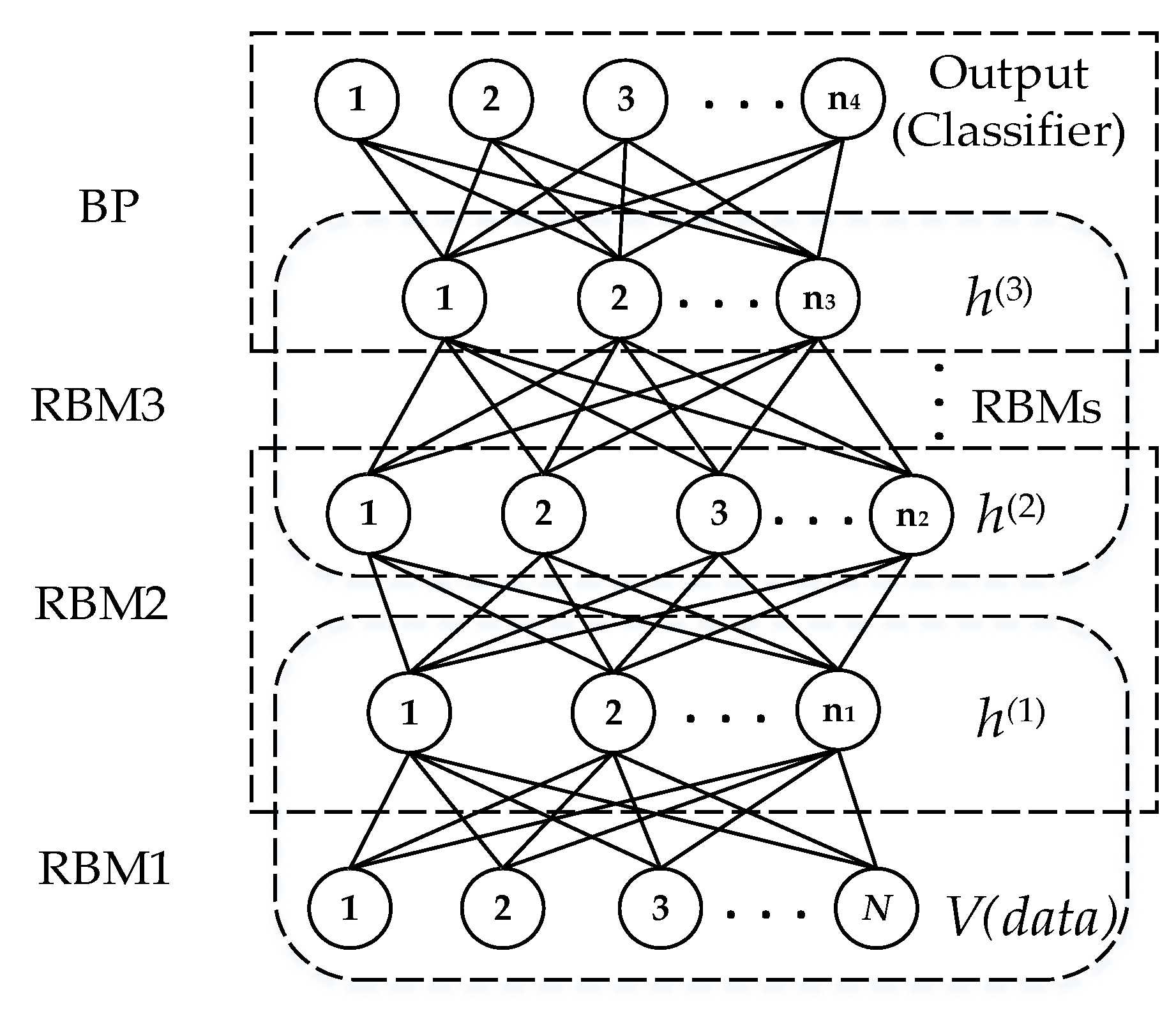
2.2. Fault Feature Classification Based on DBN

Deep belief network is one of the common methods in deep learning. DBN was first proposed by Geomey Hinton in 2006 as a multiple hidden layer probability generation model composed of multiple restricted Boltzmann machines (RBMs) [25]. Input the original data from the bottom of the network, and gradually and deeply explore the characteristics of the data from low level to high level, from concrete to abstract through layers of stacked RBM, which can not only learn the probability distribution of the data, but also classify the data.

RBM is a random binary two-layer neural network. The lower layer is the input layer, also known as the visual layer, while the top layer is the output layer, v = {v₁, v₂, …, v_m} is the state of the visual layer, and h = {h₁, h₂, …, h_n} represents the state of the hidden layer. The RBM structure diagram is shown in Figure 8.

In addition, the energy function of RBM is expressed as follows:

$$E(v,h|\theta )=-{\displaystyle \sum _{i=1}^n{a}_i{v}_i-}{\displaystyle \sum _{j=1}^m{b}_j{h}_j-}{\displaystyle \sum _{i=1}^n{\displaystyle \sum _{j=1}^m{v}_i{h}_j{w}_{ij}}}$$

(4)

where θ = {w_ij, a_i, b_j} is the parameter of the RBM model, and these parameters can be initialized randomly with minimum values; n is the number of neurons in the visible layer; and m is the number of neurons in the hidden layer.

According to Equation (4), the joint probability distribution between the visible layer and the hidden layer can be obtained:

$$\begin{array}{l}P(v,h|\theta )=\frac{1}{Z(\theta )}\exp (-E_{\theta }(v,h)),\\ Z(\theta )={\displaystyle \sum _v{\displaystyle \sum _h\exp (-E_{\theta }(v,h))}}.\end{array}$$

(5)

where Z(θ) is the normalization function.

The DBN structure for fault classification is shown in Figure 9. The DBN network is composed of multiple stacked RBMs, and the last layer is the back propagation (BP) neural network.

The process of classifying faulty data with DBN can be divided into two parts: the first part is the pre-training phase, in which the RBM is pre-trained unsupervised from bottom to top layer by layer by the CD algorithm to ensure the optimal mapping of feature vectors in the layer, thus maximizing the retention of the original feature information; the second part is the fine-tuning phase. After multiple RBMs are trained layer by layer, the obtained characteristic signals are input to the Softmax layer through a fully connected network. The BP algorithm and the sample label are used to fine tune the whole network with the cross entropy conjugate gradient descent algorithm to obtain the weight parameters of the network [26,27], so as to establish the complex mapping relationship between data features and data labels, and realize the classification function of DBN.

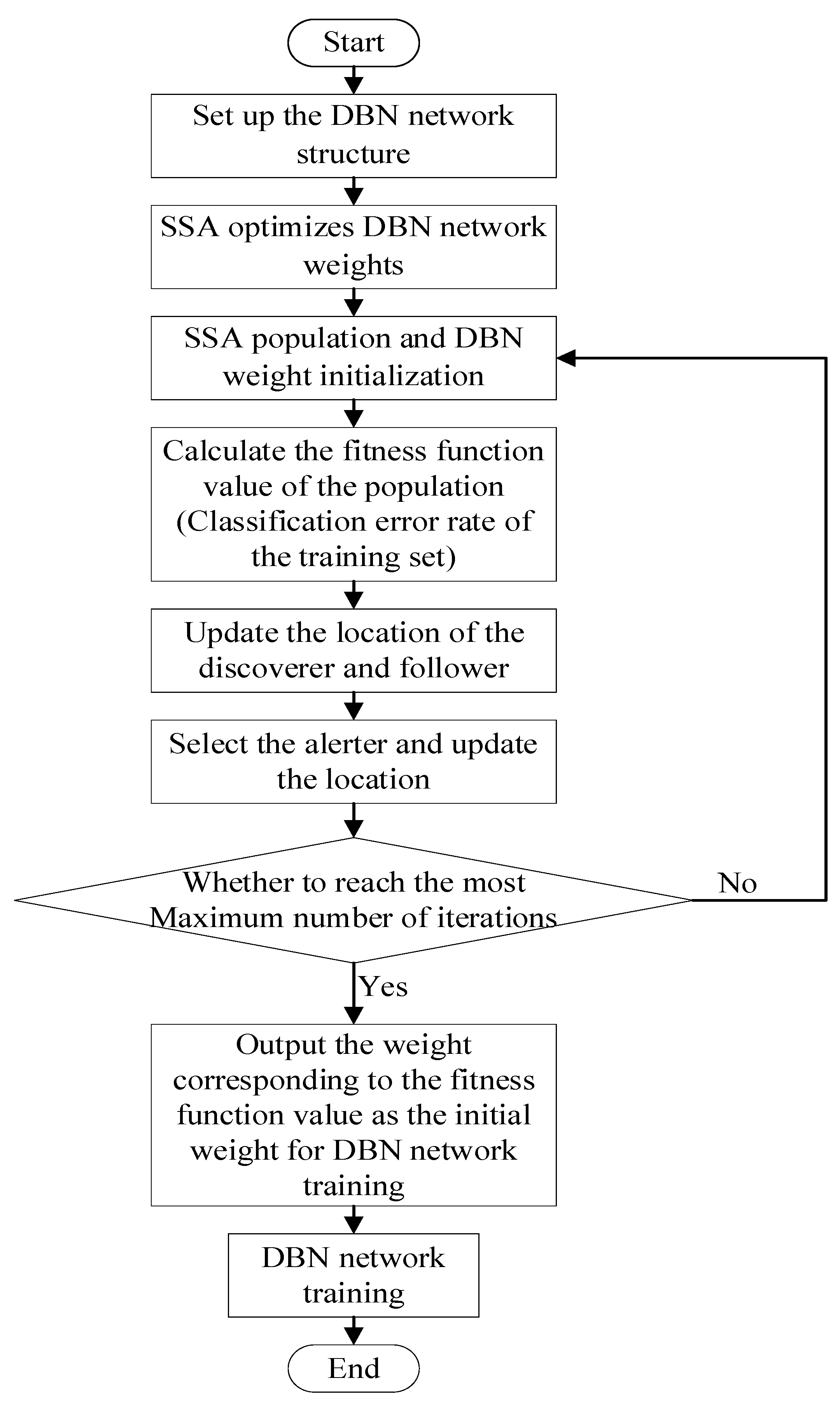
2.3. Fault Feature Classification Based on SSA-DBN

In practical application, DBN often initializes the weight value of the network randomly, which is not conducive to the update of the network weight, but also affects the classification accuracy of the network. SSA is used to optimize the weight parameters of DBN, so that it can adaptively determine the initial weight of the network, so as to effectively improve the classification accuracy and efficiency.

Sparrow search algorithm (SSA) is a swarm intelligent optimization algorithm that simulates the foraging and anti-predation behavior of sparrows. It has the advantages of strong optimization ability and fast convergence speed [28,29]. The algorithm divides the sparrows in foraging into food discoverers, accessors, and early warning.

Set the virtual sparrow population as follows:

$$X=\left[\begin{array}{cccc}{x}_{1,1}& x_{1,2}& \cdots & x_{1,d}\\ x_{2,1}& x_{2,2}& \cdots & x_{2,d}\\ \cdots & \cdots & \cdots & \cdots \\ x_{n,1}& x_{n,2}& \cdots & x_{n,d}\end{array}\right]$$

(6)

where d represents the number of variables of the problem to be optimized and n represents the number of sparrows.

Set the sparrow fitness value as follows:

$$F_X=\left[\begin{array}{c}\dot{f}\left(\left[\begin{array}{cccc}{x}_{1,1}& x_{1,2}& \cdots & x_{1,d}\end{array}\right]\right)\\ \dot{f}\left(\left[\begin{array}{cccc}{x}_{2,1}& x_{2,2}& \cdots & x_{2,d}\end{array}\right]\right)\\ \cdots \\ \dot{f}\left(\left[\begin{array}{cccc}{x}_{n,1}& x_{n,2}& \cdots & x_{n,d}\end{array}\right]\right)\end{array}\right]$$

(7)

where $\dot{f}$ represents the fitness function.

Set the discoverer’s location update formula as follows:

$$X_{i,j}^{t+1}=\{\begin{array}{r}{X}_{i,j}^t\cdot \exp (-\frac{i}{\alpha \cdot ite{r}_{\max }}),if R_2<ST\\ X_{i,j}^t+Q\cdot L, if R_2\ge ST\end{array}$$

(8)

where $t$ represents current iterations; $ite{r}_{max}$ represents the maximum number of iterations; j = 1, 2, 3, …, d; X_i,j represents the position information of the ith sparrow in the jth dimension; $\mathsf{\alpha }\in (0,1]$ is a random number; R₂ and ST represent early warning value and safety valuem respectively, and $R_2\in [0, 1]$ and $\mathit{ST}\in [0.5, 1]$; Q is a random number subject to normal distribution; and L is a 1 × d matrix with element 1.

When R₂ < ST, it means that there is no predator, and the discoverer can search for food safely. When R₂ ≥ ST, it means that predators were found, and the sparrows flew away and moved to a safe area.

Set the participants’ location update formula as follows:

$$X_{i,j}^{t+1}=\{\begin{array}{l}Q\cdot \exp \left(-\frac{X_{worst}-X_{i,j}^t}{\alpha \cdot ite{r}_{\max }}\right){,}_{}i>\frac{n}{2}\\ X_P^{t+1}+\left|X_{i,j}^t-X_P^{t+1}\right|\cdot A^{+}\cdot L{,}_{}i\le \frac{n}{2}\end{array}$$

(9)

where X_p denotes the optimal position occupied by the current discoverer; X_worst denotes the current global worst position; and A denotes a 1 × d matrix in which each element is randomly assigned 1 or −1, and A⁺ = A^T(AA^T)⁻¹. When i > n/2, it shows that the ith participant needs to forage in other areas owing to the low fitness value.

Set the location update formula of early warning person as follows:

$$X_{i,j}^{t+1}=\{\begin{array}{l}{X}_{best}^t+\beta \cdot \left|X_{i,j}^t-X_{best}^t\right|{,}_{}{f}_i>f_g\\ X_{i,j}^t+K\cdot \frac{\left|X_{i,j}^t-X_{best}^t\right|}{(f_i-f_w)}{,}_{}{f}_i=f_g\end{array}$$

(10)

where X_best denotes the optimal position occupied by the current discoverer; X_worst denotes the current global worst position; and A denotes a 1 × d matrix in which each element is randomly assigned 1 or −1, and A⁺ = A^T(AA^T)⁻¹. When i > n/2, it shows that the ith participant needs to forage in other areas owing to the low fitness value.

Set the location update formula of early warning as follows:

$$X_{i,j}^{t+1}=\{\begin{array}{l}{X}_{best}^t+\beta \cdot \left|X_{i,j}^t-X_{best}^t\right|{,}_{}{f}_i>f_g\\ X_{i,j}^t+K\cdot \frac{\left|X_{i,j}^t-X_{best}^t\right|}{(f_i-f_w)+\epsilon }{,}_{}{f}_i=f_g\end{array}$$

(11)

where X_best denotes the current global optimal location; β denotes a random number that obeys the standard normal distribution; $K\in [-1, 1]$ denotes the direction of sparrow movement as well as a step control parameter; f_i denotes the current sparrow fitness value; f_g and f_w denote the current global optimal and worst fitness values; and ε denotes a minimal constant.

When f_i > f_g, it indicates that the early warning is located at the edge of the population and needs to move to a safe area. When f_i > f_g, it means that the early warning is aware of the danger and needs to be close to other sparrows.

The flow chart of fault feature classification based on SSA-DBN is shown in Figure 10. When the number of iterations reaches the preset maximum number of iterations, the weight corresponding to the fitness function value is output as the initial weight of DBN network training for DBN network training.

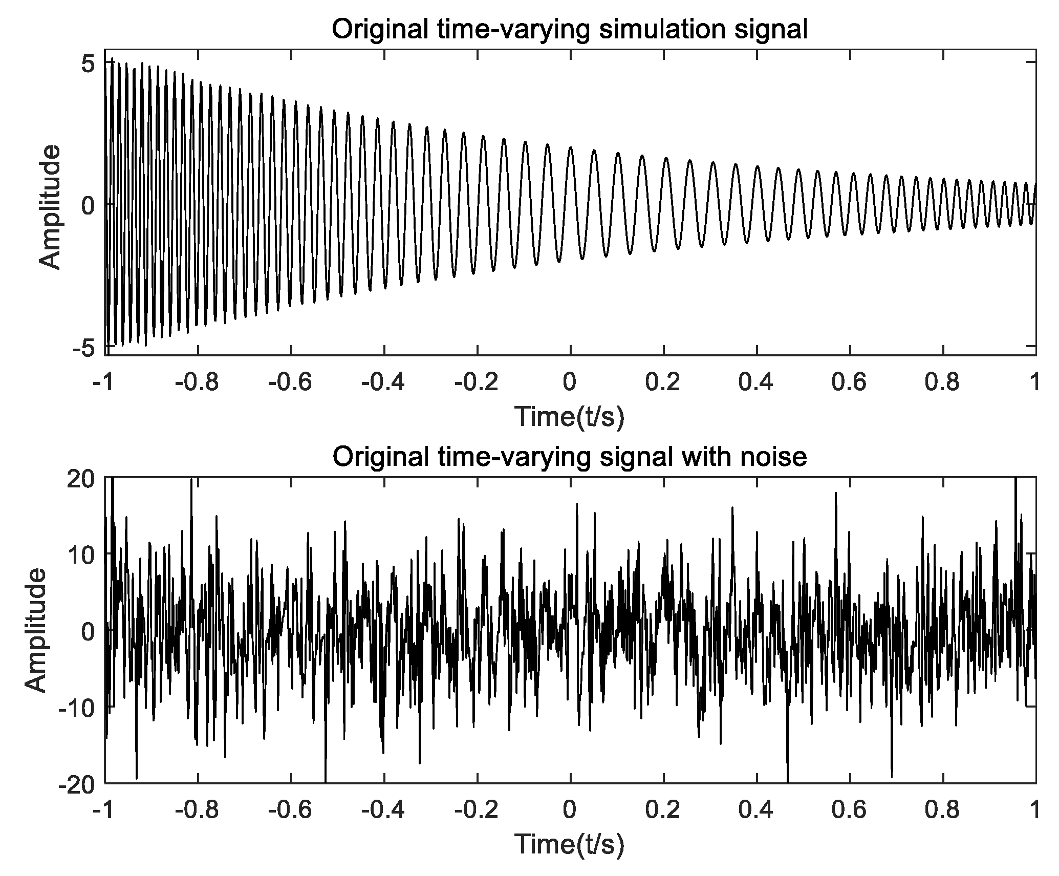
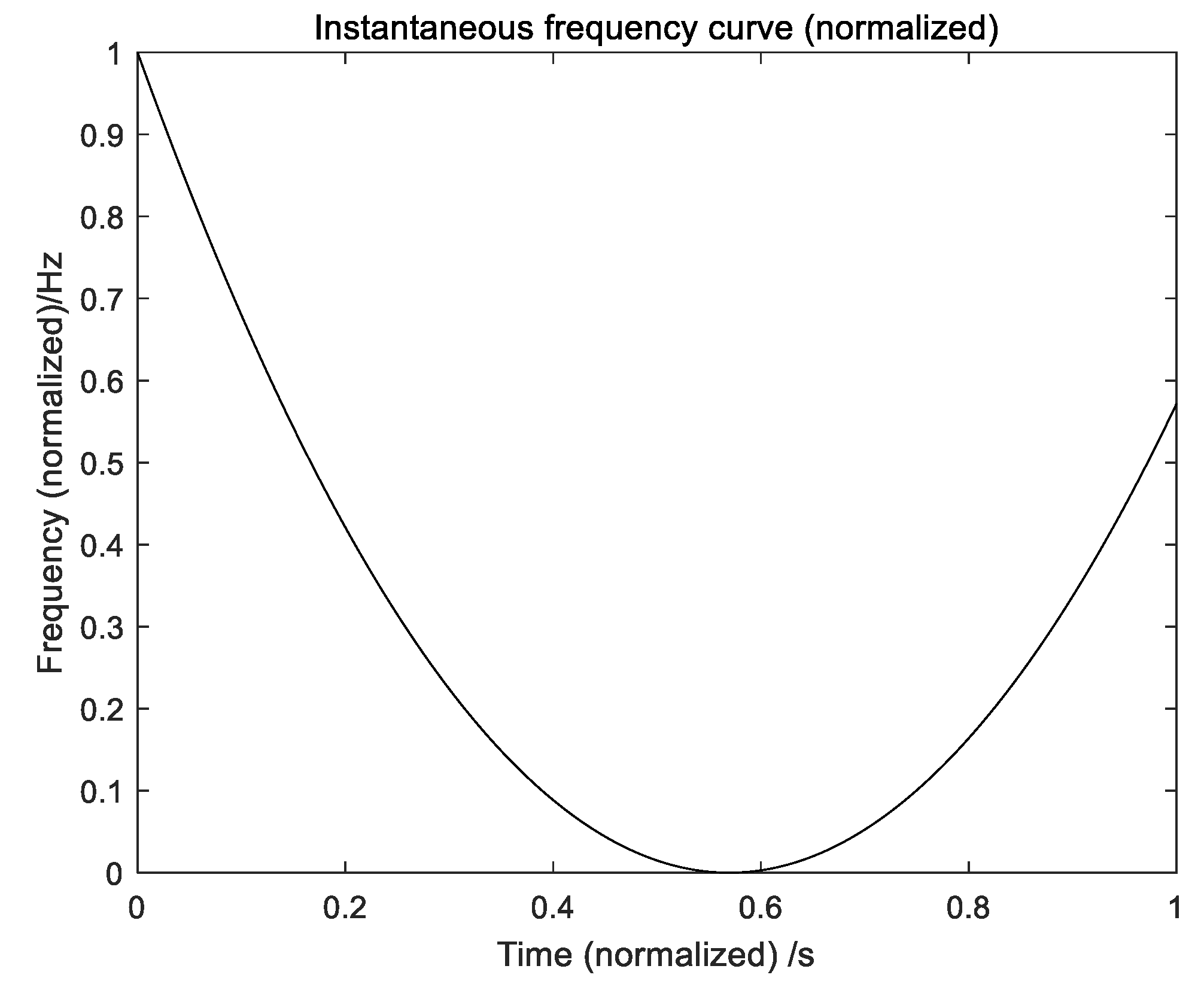
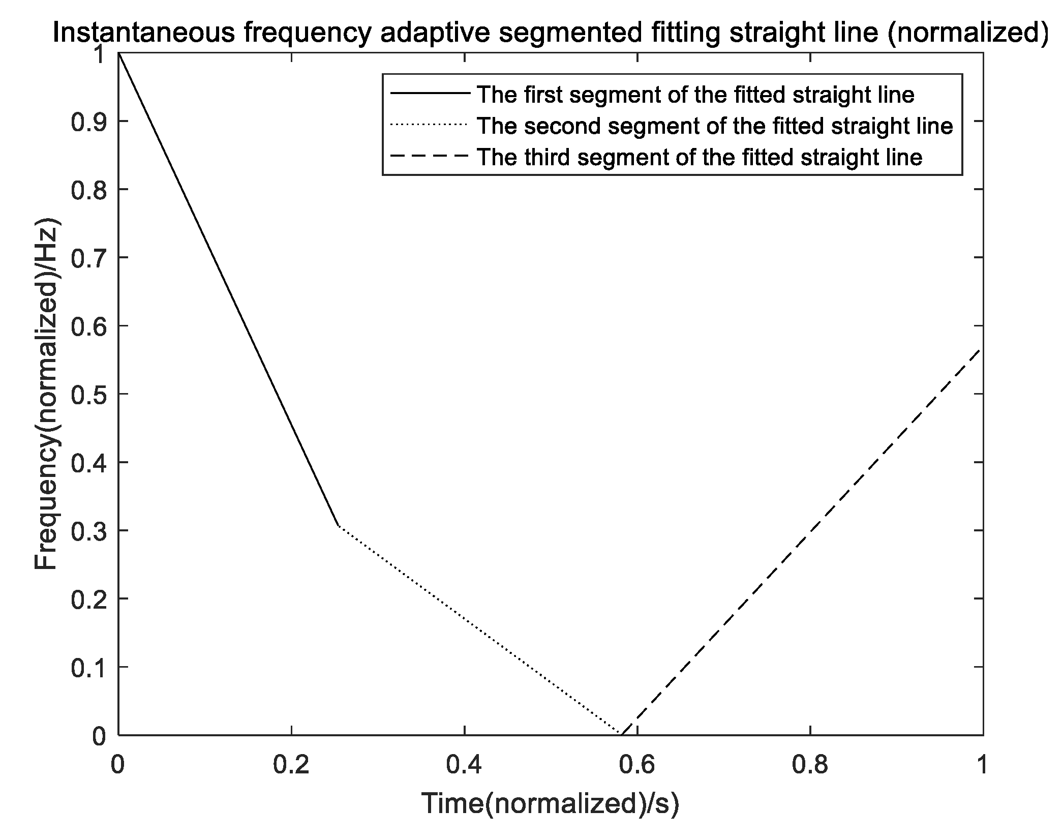
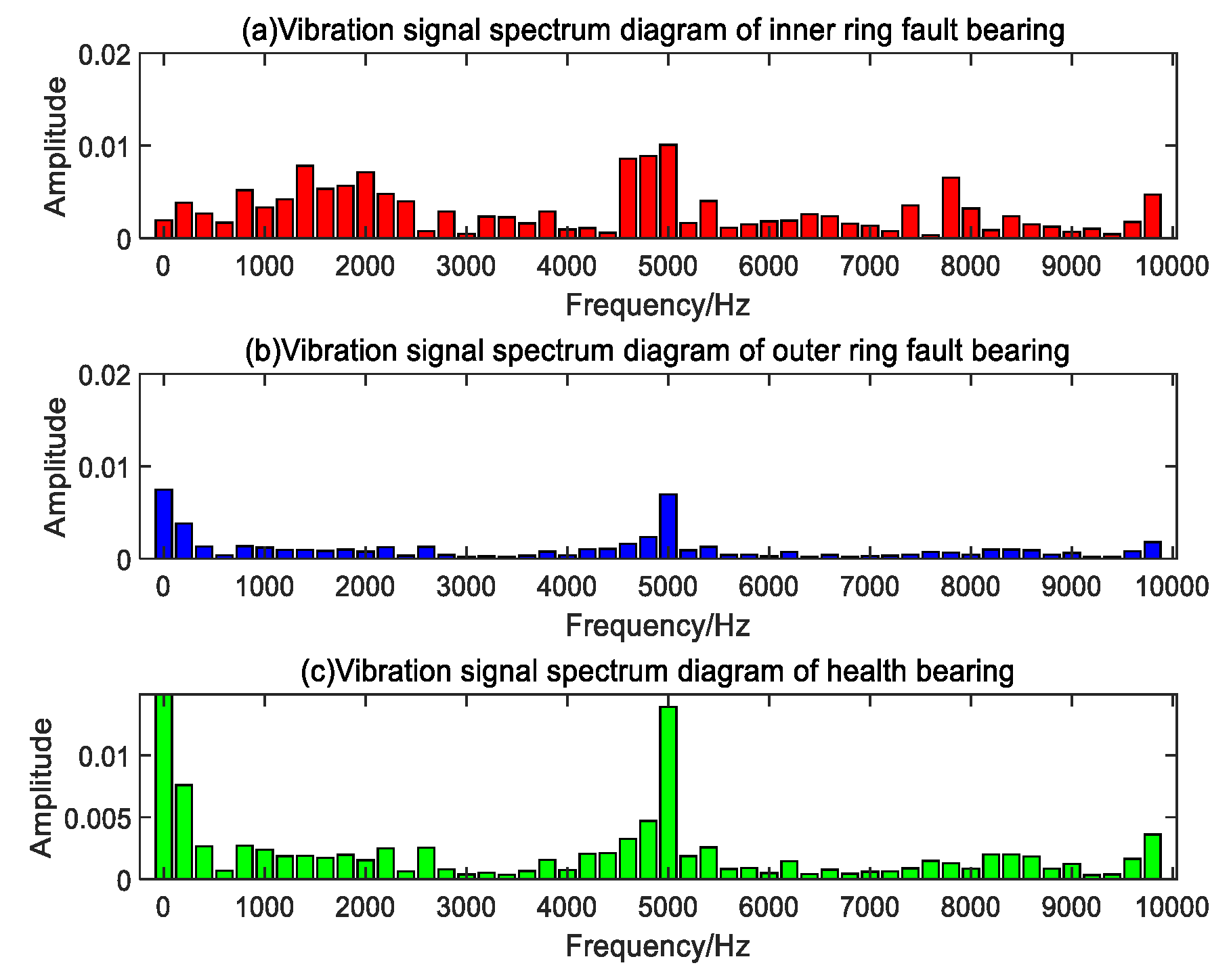
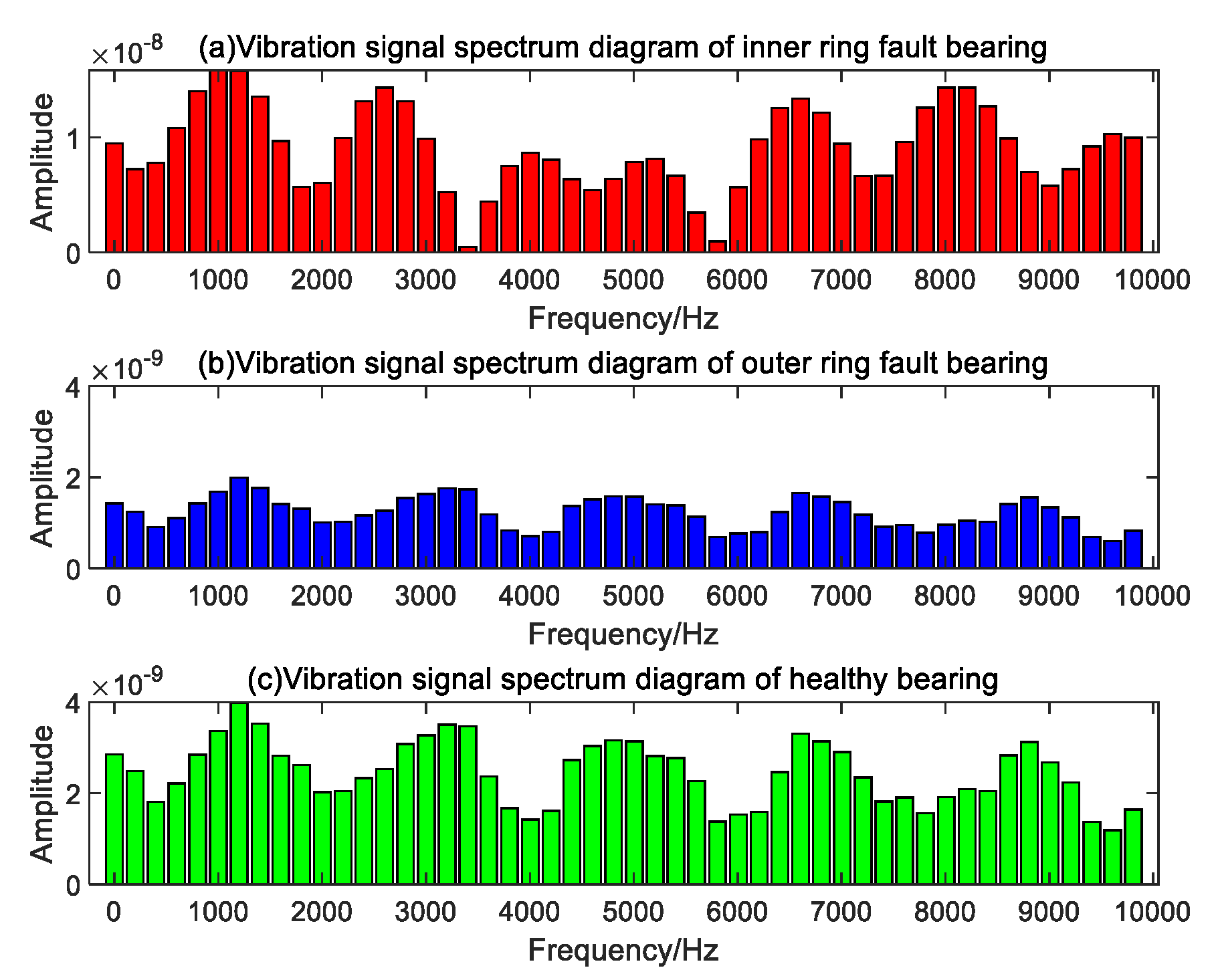
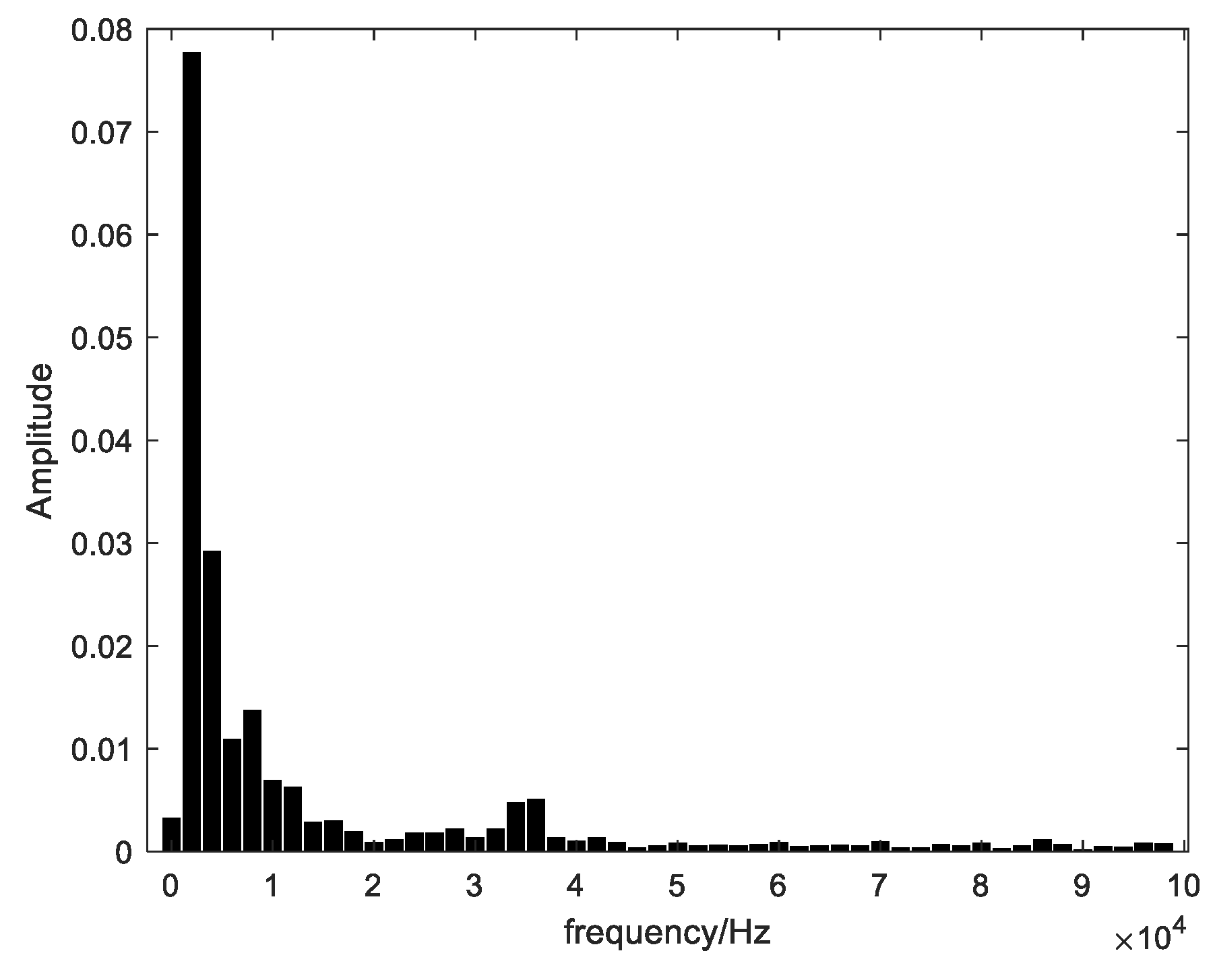
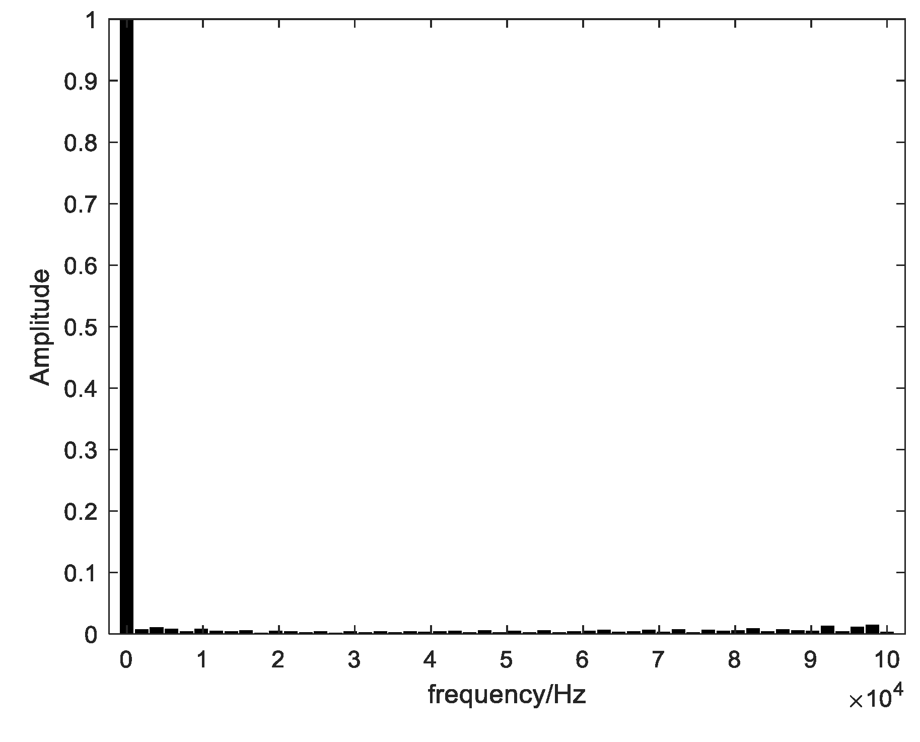
3. Experimental Result

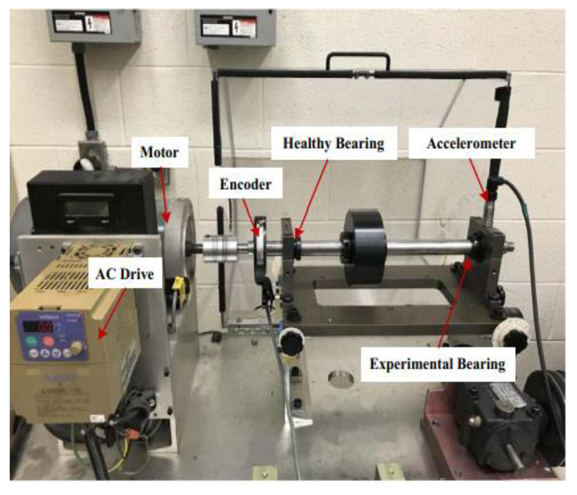
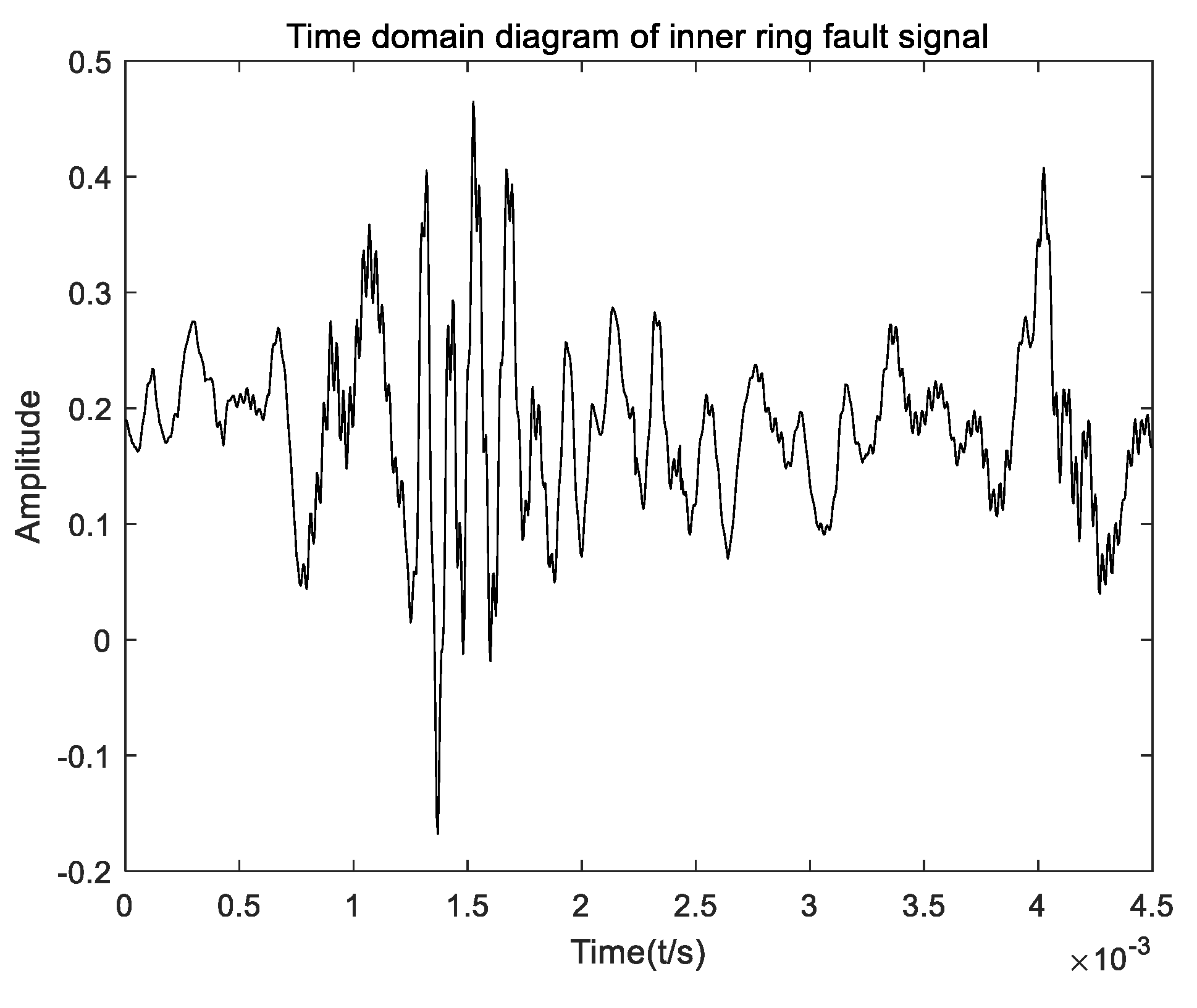
3.1. Data Description

The validation data used in this paper are from the rotating machinery fault simulator MKF-PK5M in the laboratory of the University of Ottawa, as shown in Figure 11. The spindle is driven by a motor and the speed is controlled by an AC driver. Two er16k ball bearings are installed to support the shaft. The acceleration sensor is installed on the shell of the left experimental bearing to collect vibration data. In addition, a tachometer (EPC 775) is installed to measure the speed of the shaft. The data are collected by Ni data acquisition board (NI USB-6212 BNC) and recorded by computer software LabVIEW [30]. The sampling frequency is 200,000 Hz and the sampling time is 10 s.

The experimental bearings are divided into bearings with inner ring defects, bearings with outer ring defects, and healthy bearings. See

Table 1. Bearing parameters.

Bearing Type	Pitch Diameter	Rolling Element Diameter	Number of Balls	FCCi 1	FCCo 2
ER16K	38.53 mm	7.94 mm	9	5.43fr	3.57fr

¹ FCC_i is the fault characteristic coefficient of inner ring. ² FCC_o is the fault characteristic coefficient of outer ring.

for details of their parameters. The running state of the bearing is divided into three categories: speed increase, speed decrease, and speed increase first and then decrease. In this simulation experiment, the operating state with increased bearing speed is selected, and the number of sampling points is 16384, which is more than the number of points collected during one week of bearing operation, so it can include all fault characteristics of the bearing under its corresponding health condition.

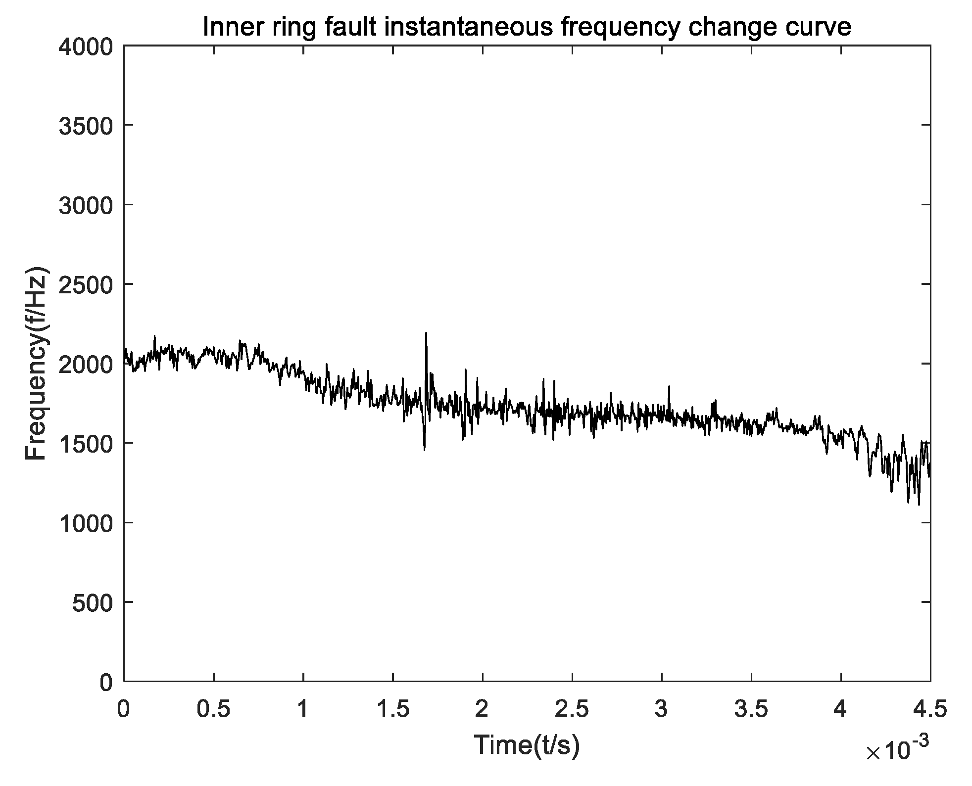
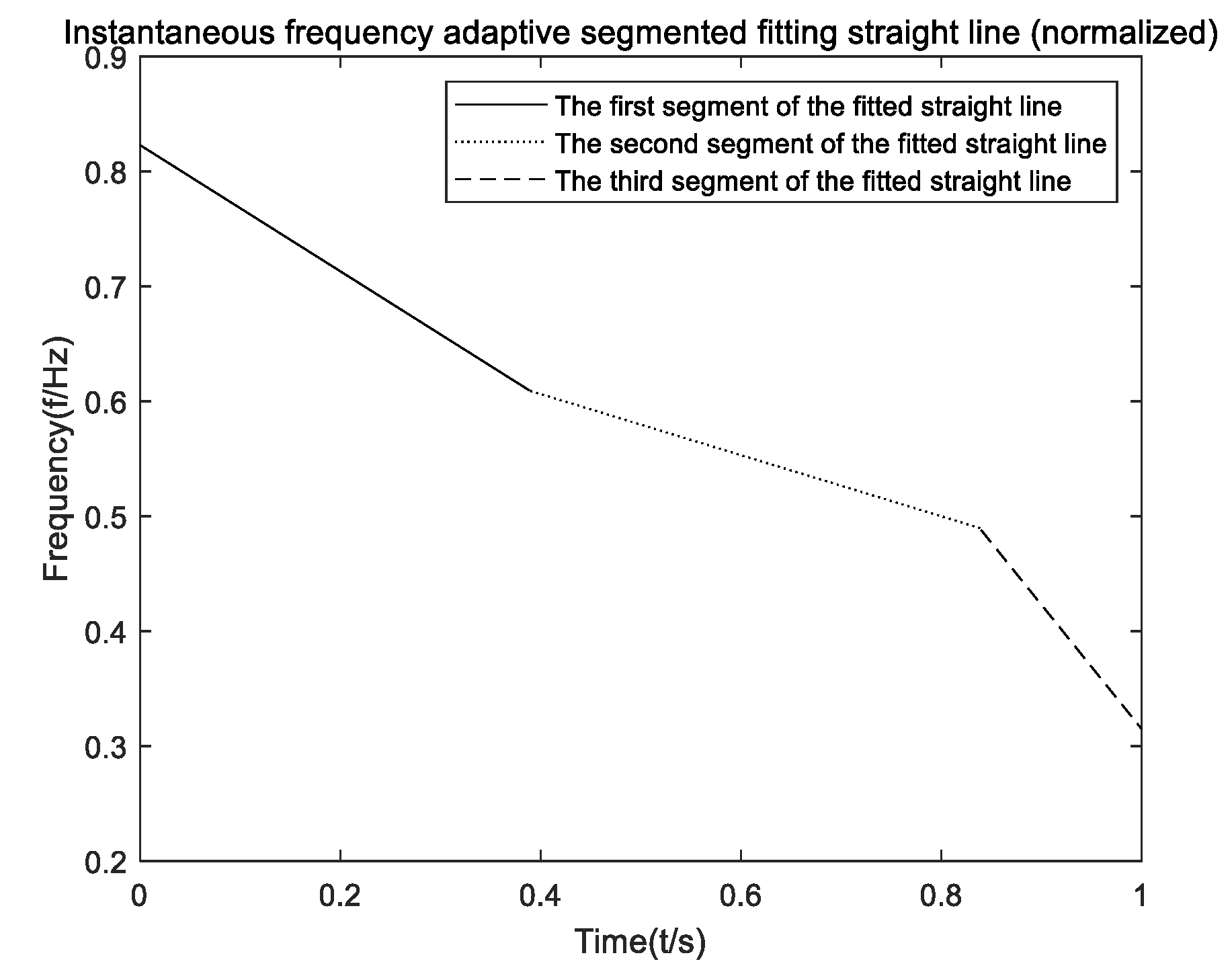
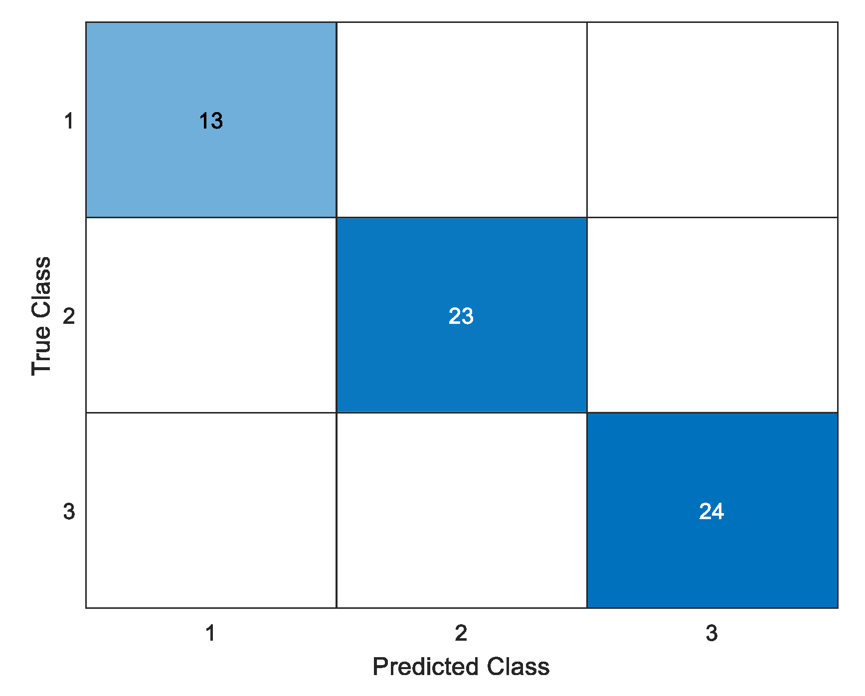
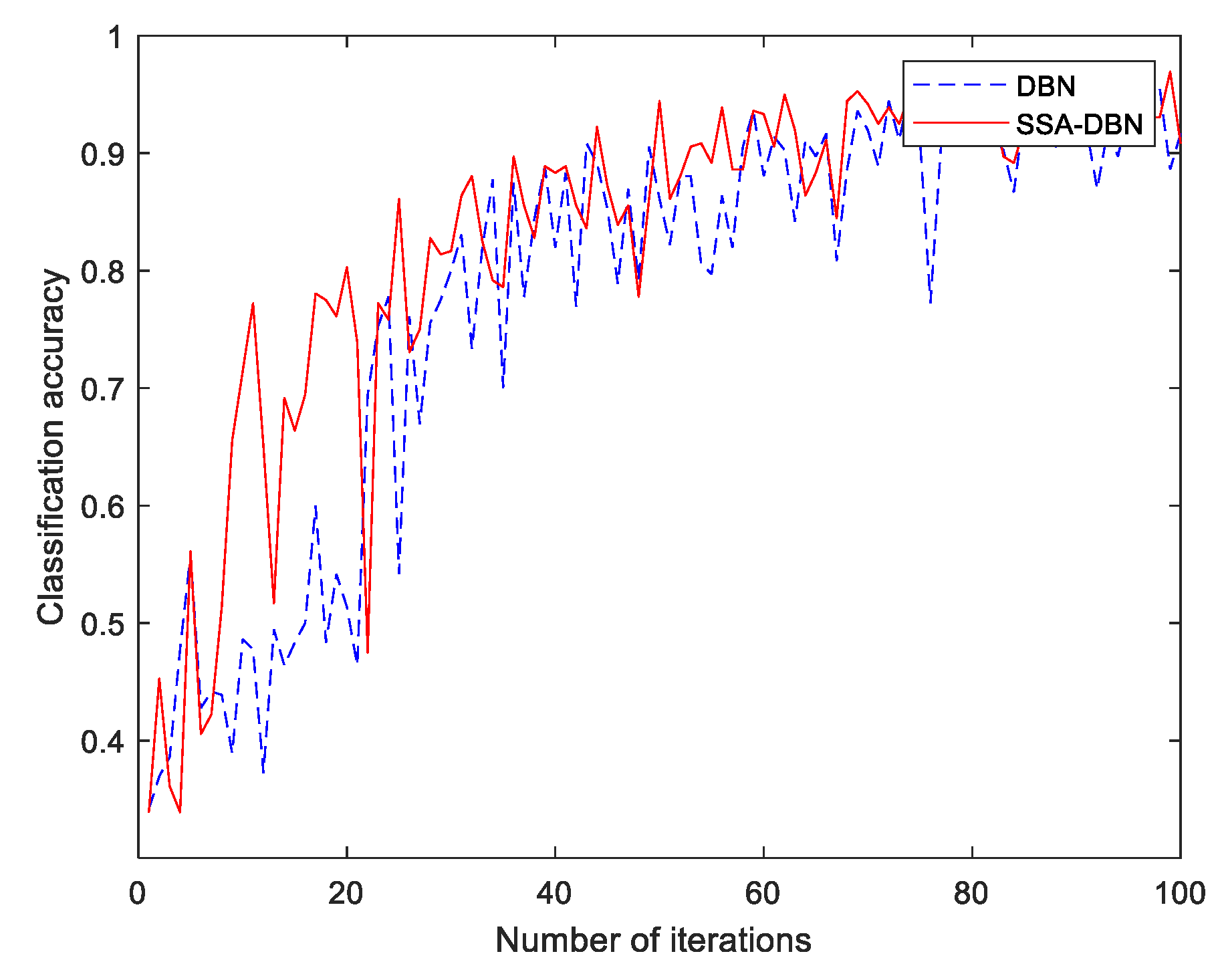
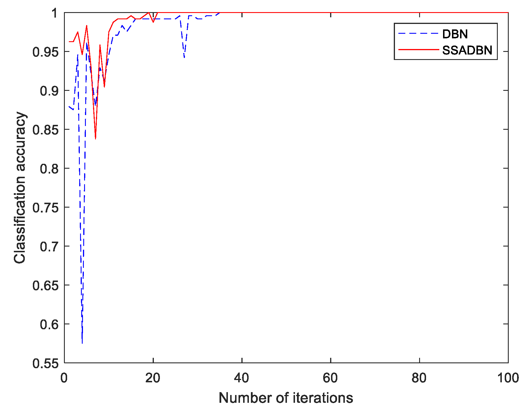
3.2. Condition Monitoring of the Rolling Bearing under Variable Speeds

The process of condition monitoring method based on curve feature segmentation multi-order FRFT filtering and SSA-DBN classification and recognition is shown in Figure 12.

The vibration signal is filtered by segmented multi-order FRFT based on curve features to extract the early fault characteristic frequency of rolling bearing. The rolling bearing with defective inner ring is selected for simulation analysis of fault characteristic frequency extraction.

The calculation formula of fault characteristic frequency f_ic is as follows:

$$\begin{array}{l}{f}_{ic}=\frac{Z}{2}(1+\frac{d}{D}\cos \alpha )f_r,\\ FCC=\frac{Z}{2}(1+\frac{d}{D}\cos \alpha ).\end{array}$$

(12)

where Z is the number of balls, d is the diameter of rolling element, D is the pitch diameter, f_r is the rotation frequency of bearing, and α is the rotation angle.

It can be seen that the bearing fault characteristic coefficient FCC is only related to its own structural parameters and has nothing to do with the change in speed. Therefore, the type of bearing fault under variable speed can be judged by comparing the ratio of fault characteristic frequency and shaft rotation frequency with the theoretical value of fault characteristic coefficient. The rotation frequency change is 12.5~27.8 Hz. The time domain diagram of inner ring fault signal is shown in Figure 13.

Firstly, estimate the instantaneous frequency curve of vibration signal. The EMD algorithm is used to adaptively decompose the vibration signal. The components IMF2, IMF3, and IMF4 with large correlation with the original signal are selected by the correlation coefficient method for signal reconstruction. The instantaneous frequency curve is extracted from the reconstructed signal by the method based on the phase information of Morlet wavelet coefficients, as shown in Figure 14.

Then, piecewise multi-order FRFT filtering based on curve features is carried out. The instantaneous frequency curve shall be combined and normalized, as shown in Figure 15. According to many experiments, the curvature thresholds are set to 0.00098 and 0.00192, respectively, and the normalized instantaneous frequency curve is adaptively segmented according to the curvature threshold. The least squares method is used to fit the frequency curve of each section, as shown in Figure 16. Then, the frequency modulation rate of each segment is f_m1 = −0.5491, f_m2 = −0.2658, and f_m3 = −1.0802, and then the optimal order of each segment is p₁ = 0.6803, p₂ = 0.8346, and p₃ = 0.4755 using the following formula.

$$p_i=1+\frac{2}{\pi }\arctan f_{mi}$$

(13)

The FRFT transform of corresponding order is carried out for each section of signal, and the results are shown in Figure 17, Figure 18 and Figure 19. It can be seen that the peak value of each section of signal appears at u₁ = 246, u₂ = 214, and u₃ = 36. Therefore, the narrowband pass filter is designed with u₁, u₂, and u₃ as the filtering center. Finally, the fault characteristic frequency of the signal is extracted using a 1.5-dimensional Teager energy spectrum, as shown in Figure 20.

As can be seen from Figure 20, the frequency value corresponding to the maximum amplitude is 132.7 Hz. Therefore, the characteristic frequency value of inner ring fault is 132.7 Hz. According to the speed information collected from the experiment, the shaft rotation frequency corresponding to this section of data is 24.4 Hz. Therefore, according to the formula FCC = f_{ic /} f_r, the fault characteristic coefficient can be calculated as 5.4385, which is equal to the theoretical value of the fault characteristic coefficient of the bearing inner ring. It is verified that the multi-order FRFT based on curve features can accurately extract the fault characteristic frequency of rolling bearing under variable speeds.

Select 300 samples respectively for the signals filtered by FRFT in each state segment, and the length of each sample is 864. See

Table 2. Division of data sets.

Dataset Number	Fault Type	Number of Training Samples	Number of Test Samples	Fault Tag
1	Inner ring fault	240	60	001
2	Outer ring fault	240	60	010
3	Healthy bearing	240	60	100

for the specific division of the data set.

Different preprocessing will be carried out on the data set to test the effectiveness of SSA-DBN, because the spectrum characteristics of bearing vibration signals can better characterize the characteristics of different fault types. The constructed data sets are divided into two types: the first is the spectrum data set obtained by FFT transformation of the original time-domain signal, as shown in Figure 21; the second is the spectrum data set composed of FFT after multi-order FRFT filtering, as shown in Figure 22. Figure 23 and Figure 24 describe the input samples of the first and second data sets, respectively.

DBN parameter setting: according to experience, the DBN network is tested under different layers, nodes, and iteration times according to the principle of step-by-step decreasing to facilitate feature extraction. The network structure is 432-50-20-3, the pre-training learning rate is 0.6, the reverse fine tuning learning rate is 0.01, the cross entropy is used as the loss function, and the maximum number of iterations is 1000.

SSA parameter settings: when the input sample is the FFT amplitude of the original time domain signal, the population size is set to 10, the number of discoverers accounts for 10% of the whole population, the number of sparrows aware of the danger SD = 2, the safety threshold st = 0.8, and the maximum number of iterations is 10. When the input sample is the FFT amplitude of the multi-order FRFT filtered signal, the population size is set to 15, the number of discoverers accounts for 20% of the whole population, the number of sparrows aware of the danger SD = 2, the safety threshold ST = 0.85, and the maximum number of iterations is 10.

Both input samples take the classification error rate of the training set as the fitness function, and the change process of the fitness function is shown in Figure 25 and Figure 26. As can be seen from Figure 25, when the number of iterations is greater than or equal to 6, the classification error rate of the network reaches the minimum value of 2.5%. Therefore, the corresponding weight parameters are selected as the initial weight of the DBN model to train the network.

The classification results of the training model on the test set are shown in Figure 27, in which the abscissa represents the bearing state predicted by the network and the ordinate represents the real state of the bearing. The box on the diagonal represents the number of test samples with the same predicted state and real state, and the numbers in the other boxes represent the number of misclassified samples. When the input sample is the FFT amplitude of the original time domain signal, the classification accuracy of other categories is 100%, except that three samples with inner ring fault are wrongly diagnosed as outer ring fault, so SSA-DBN has high classification accuracy.

As can be seen from Figure 26, when the number of iterations is 9, the fitness function value reaches the minimum value of 15%. Therefore, the corresponding weight parameter is selected as the initial weight of the DBN model to train the network. The classification results of the training model on the test set are shown in Figure 28. The simulation results show that, when the input sample is the FFT amplitude of the multi-order FRFT filtered signal, the fault state of each test sample can be accurately identified, which shows that SSA-DBN has strong fault type identification ability.

To illustrate the optimization effect of SSA on DBN and the effectiveness of the multi-order FRFT filtering method based on curve feature segmentation, the diagnostic results are summarized in

Table 3. Classification results of different diagnostic models.

Input Sample	SSA-DBN		DBN		BP		SVM
	Accuracy	Time	Accuracy	Time	Accuracy	Time	Accuracy	Time
Spectrum of original signal	95%	106.57 s	91.2%	99.48 s	70%	0.61 s	55%	1.04 s
Spectrum of multi-order FRFT filtered signal	100%	104.54 s	96.38%	104.21 s	98.33%	3.48 s	83.33%	0.53 s

by comparing them with DBN, BP neural network, and the support vector machine (SVM) models with the same input samples.

As can be seen from Table 3, when the input sample sets are different, the classification accuracy of SSA-DBN is higher than that of DBN, BP, SVM, and other models, and they are more than 95% or even 100%. In addition, the simulation time of SSA-DBN is slightly higher than that of DBN and other models. It can be seen that SSA can improve the classification accuracy of DBN on the basis of ensuring the simulation time. In the two diagnostic models, the classification accuracy of the network trained with multi-order FRFT filtered signal is higher than that of the network not trained with filtered signal, which shows the effectiveness of the multi-order FRFT filtering algorithm. Finally, in order to illustrate the optimization effect of SSA on DBN again, the change process of accuracy rate of DBN and SSA-DBN models during training is selected for analysis, and the change curve of classification accuracy rate of training network with different input samples is shown in Figure 29 and Figure 30.

As can be seen from Figure 29 and Figure 30, in the process of network training, when the input samples of the model are different, the classification accuracy of SSA-DBN model is higher than that of DBN model. In addition, it can be seen from Figure 30 that, when the accuracy of network classification is greater than 95%, the number of iterations of SSA-DBN model is less than that of DBN model, and the stability is good. In conclusion, SSA can accelerate the training speed of DBN model and has better stability.

4. Conclusions

Aiming at the difficulties of early fault feature extraction and classification identification of variable speed bearings under strong background noise, a condition monitoring method based on a piecewise multi-order FRFT filter with curve features and SSA-DBN classification identification method is proposed. Its main innovation points can be summarized as follows. (1) The multi-order FRFT filtering algorithm based on the slice of curve features is adopted to effectively obtain fault characteristics from the original signal under severe interference by noise; (2) the sparrow search algorithm is used to optimize each weight parameter of DBN so that it can adaptively determine the initial model parameters, which can effectively improve the classification accuracy and classification efficiency and meet the demand of real-time diagnosis.

The vibration data of the faulty bearing at the drive end of the motor in the bearing dataset of the University of Ottawa are used as the experimental sample for the experiments when the speed increases approximately linearly. The simulation shows that the binned multi-order FRFT filter based on curve features, which linearizes signals with nonlinear frequencies and filters them in the binned domain, can effectively filter noise and accurately extract fault characteristic frequencies; furthermore, SSA-DBN is used to classify and identify early bearing faults. The classification accuracy of SSA-DBN is higher than that of DBN, reaching more than 95% or even 100%. Therefore, the proposed method can not only accurately extract the early fault feature information of variable speed bearings, but also has high classification accuracy.

References

1. Ma, J.P.; Zhuo, S.; Li, C.W.; Zhan, L.W.; Zhang, G.Z. An enhanced intrinsic time-scale decomposition method based on adaptive lévy noise and its application in bearing fault diagnosis. Symmetry 2021, 13, 617. [Google Scholar] [CrossRef]
2. Gao, S.Z.; Li, T.C.; Zhang, Y.M. Rolling bearing fault diagnosis of PSO-LSSVM based on CEEMD entropy fusion. Trans. Can. Soc. Mech. Eng. 2020, 44, 405–418. [Google Scholar] [CrossRef]
3. He, X.; Ma, J. Weak fault diagnosis of rolling bearing based on FRFT and DBN. Syst. Sci. Control Eng. 2020, 8, 57–66. [Google Scholar] [CrossRef]
4. Li, C.; Liang, M.; Chen, Z.Q.; Bai, Y. Intelligent Health Management of Rolling Bearing Based on Vibration Signal; Science: Beijing, China, 2018. [Google Scholar]
5. Hao, X.Y.; Zheng, Y.; Lu, L.; Pan, H. Reaearch on intelligent fault diagnosis of rolling bearing based on improved deep residual network. Appl. Sci. 2021, 11, 10889. [Google Scholar] [CrossRef]
6. Rostaghi, M.; Khatibi, M.M.; Ashory, M.R.; Azami, H. Bearing fault diagnosis using refined composite generalized multiscale dispersion entropy-based skewness and variance and multiclass FCM-ANFIS. Symmetry 2021, 23, 1510. [Google Scholar] [CrossRef]
7. Chen, F.F.; Cheng, M.T.; Tang, B.P.; Chen, B.J.; Xiao, W.R. Pattern recognition of a sensitive feature set based on the orthogonal neighborhood preserving embedding and adaboost_SVM algorithm for rolling bearing early fault diagnosis. Meas. Sci. Technol. 2020, 31, 105007. [Google Scholar] [CrossRef]
8. Wang, H.; Chen, J.H.; Zhou, Y.W.; Ni, G.X. Early fault diagnosis of rolling bearing based on noise-assisted signal feature enhancement and stochastic resonance for intelligent manufacturing. Int. J. Adv. Manuf. Technol. 2020, 107, 1017–1023. [Google Scholar] [CrossRef]
9. Li, Y.B.; Yang, Y.T.; Wang, X.Z.; Liu, X.Z.; Liu, B.B.; Liang, X.H. Early fault diagnosis of rolling bearings based on hierarchical symbol dynamic entropy and binary tree support vector machine. J. Sound. Vib. 2018, 428, 72–86. [Google Scholar] [CrossRef]
10. Li, J.; Zhou, D.H.; Si, X.S.; Chen, M.Y.; Xu, C.H. Review of incipient fault diagnosis methods. Control Theory Appl. 2012, 29, 1517–1528. [Google Scholar]
11. Zhao, X.P.; Wang, Y.F.; Zhang, Y.H.; Wu, J.X.; Shi, Y.Q. Weak fault diagnosis of rolling bearing based on improved stochastic resonance. CMC-Comput. Mater. Con. 2020, 64, 571–587. [Google Scholar] [CrossRef]
12. Xu, L.; Chatterton, S.; Pennacchi, P. Rolling element bearing diagnosis based on singular value decomposition and composite squared envelope spectrum. Mech. Syst. Signal Pract. 2021, 148, 107174. [Google Scholar] [CrossRef]
13. Wen, C.L.; Lv, F.Y.; Bao, Z.J.; Liu, M.Q. A Review of Data Driven-based Incipient Fault Diagnosis. Acta Autom. Sin. 2016, 42, 1286–1299. [Google Scholar]
14. Namias, V. The fractional order Fourier transform and its application to quantum mechanics. IMA J. Appl. Math. 1980, 25, 241–265. [Google Scholar] [CrossRef]
15. Lin, L.F.; Wang, H.Q.; Lv, W.Y.; Zhong, S.C. A novel parameter-induced stochastic resonance phenomena in fractional Fourier domain. Mech. Syst. Signal Pract. 2016, 76–77, 771–779. [Google Scholar] [CrossRef]
16. Qi, L.; Tao, R.; Zhou, S.Q.; Wang, Y. Detection and parameter estimation of multicomponent LFM signals based on fractional Fourier transform. Sci. China Ser. E 2003, 33, 749–759. [Google Scholar] [CrossRef]
17. Du, X.W.; Wen, G.R.; Liu, D.; Chen, X.Y.; Zhang, Y.; Luo, J.Q. Fractional iterative variational mode decomposition and its application in fault diagnosis of rotating machinery. Meas. Sci. Technol. 2019, 30, 125009. [Google Scholar] [CrossRef]
18. Tang, G.; Huang, Y.J.; Wang, Y.T. Fractional frequency band entropy for bearing fault diagnosis under varying speed conditions. Measurement 2021, 171, 108777. [Google Scholar] [CrossRef]
19. Mei, J.M.; Xiao, Y.K. Diagnosis Technology of Fearbox’s Early Fault--Fractional Fourier Transform Principle and Applications; Higher Education Press: Beijing, China, 2016. [Google Scholar]
20. Chen, G.Y.; Yan, C.F.; Meng, J.D.; Wang, H.B.; Wu, L.X. Improved VMD-FRFT based on initial center frequency for early fault diagnosis of rolling element bearing. Meas. Sci. Technol. 2021, 32, 115024. [Google Scholar] [CrossRef]
21. Shao, Y. The application of fractional Fourier transform algorithm in signal analysis. Master’s thesis, Harbin University of Science and Technology, Harbin, China, 2016. [Google Scholar]
22. Zhu, J.; Hu, T.Z.; Jiang, B.; Yang, X. Intelligent bearing fault diagnosis using PCA-DBN framework. Neural. Comput. Appl. 2020, 32, 10773–10781. [Google Scholar] [CrossRef]
23. Qin, Y.; Wang, X.; Zou, J.Q. The Optimized Deep Belief Networks With Improved Logistic Sigmoid Units and Their Application in Fault Diagnosis for Planetary Gearboxes of Wind Turbines. IEEE Trans. Ind. Electr. 2019, 66, 3814–3824. [Google Scholar] [CrossRef]
24. Zhang, Y.H.; Zhang, Y.S.; Wen, L.B.; Cui, Z.M.; Liu, G.S. Power Grid Fault Diagnosis Based on Improved Deep Belief Network. J. Phys. Conf. Ser. 2020, 1585, 012021. [Google Scholar] [CrossRef]
25. Xu, F.; Fang, Y.J.; Wang, D.; Liang, J.Q. Combining DBN and FCM for Fault Diagnosis of Roller Element Bearings without Using Data Labels. Hindawi 2018, 2018, 1–12. [Google Scholar] [CrossRef]
26. Hinton, G.E.; Salakhutdinov, R.R. Reducing the dimensionality of data with neural networks. Science 2006, 313, 504–507. [Google Scholar] [CrossRef] [Green Version]
27. Liu, Y.L.; Yang, D.L. Bearing Fault Diagnosis Based on Deep Belief Network and Multisensor Information Fusion. Hindawi 2016, 2016, 1–9. [Google Scholar]
28. Xue, J.K.; Shen, B. A novel swarm intelligence optimization approach: Sparrow search algorithm. Syst. Sci. Contr. Eng. 2020, 8, 22–34. [Google Scholar] [CrossRef]
29. Lv, J.; Sun, W.L.; Wang, H.W.; Zhang, F. Coordinated Approach Fusing RCMDE and Sparrow Search Algorithm-Based SVM for Fault Diagnosis of Rolling Bearings. Sensors 2021, 21, 5297. [Google Scholar] [CrossRef]
30. Huang, H.; Baddour, N. Bearing vibration data collected under time-varying rotational speed conditions. Data Brief 2018, 21, 1745–1749. [Google Scholar] [CrossRef] [PubMed]
Figure 1. LFM signal extracted by FRFT.
Symmetry 14 00320 g001
Figure 2. NLFM signal extracted by FRFT.
Symmetry 14 00320 g002
Figure 3. Least squares fitting frequency band of each segment of component 1.
Symmetry 14 00320 g003
Figure 4. Time domain diagram of NLFM signal.
Symmetry 14 00320 g004
Figure 5. Instantaneous frequency curve of NLFM signal (normalized).
Symmetry 14 00320 g005
Figure 6. Instantaneous frequency curve of NLFM signal (normalized).
Symmetry 14 00320 g006
Figure 7. Time domain diagram of the filtered signal.
Symmetry 14 00320 g007
Figure 8. RBM structure.
Symmetry 14 00320 g008
Figure 9. Structure of DBN for fault classification.
Symmetry 14 00320 g009
Figure 10. Flow chart of fault feature classification based on SSA-DBN.
Symmetry 14 00320 g010
Figure 11. Diagram of the experimental set-up.
Symmetry 14 00320 g011
Figure 12. Flow chart of bearing condition monitoring under variable speeds.
Symmetry 14 00320 g012
Figure 13. Time domain diagram of inner ring fault signal.
Symmetry 14 00320 g013
Figure 14. Frequency curve extracted by Morlet wavelet transform.
Symmetry 14 00320 g014
Figure 15. Instantaneous frequency fitting curve (normalized).
Symmetry 14 00320 g015
Figure 16. Instantaneous frequency fitting curve (normalized).
Symmetry 14 00320 g016
Figure 17. FRFT result diagram of the first segment of data.
Symmetry 14 00320 g017
Figure 18. FRFT result diagram of the second segment of data.
Symmetry 14 00320 g018
Figure 19. FRFT result diagram of the third segment of data.
Symmetry 14 00320 g019
Figure 20. 1.5D Teager energy spectrum of multi-order FRFT filtered signal.
Symmetry 14 00320 g020
Figure 21. FFT spectrum of original time domain signal.
Symmetry 14 00320 g021
Figure 22. FFT spectrum of multi-order FRFT filtered signal.
Symmetry 14 00320 g022
Figure 23. Input samples for the first dataset.
Symmetry 14 00320 g023
Figure 24. Input samples for the second dataset.
Symmetry 14 00320 g024
Figure 25. Fitness curve of the original signal spectrum as the input sample.
Symmetry 14 00320 g025
Figure 26. Fitness curve of multi-order FRFT filtered signal spectrum as input samples.
Symmetry 14 00320 g026
Figure 27. Diagnosis result diagram of original time domain signal spectrum as input samples.
Symmetry 14 00320 g027
Figure 28. Diagnosis results of multi-order FRFT filtered signal spectrum as input samples.
Symmetry 14 00320 g028
Figure 29. Change curve of accuracy rate of original vibration signal sample training network.
Symmetry 14 00320 g029
Figure 30. Change curve of accuracy rate of sample training network after segmented FRFT processing.
Symmetry 14 00320 g030