The Quest for the Astrophysical Gravitational-Wave Background with Terrestrial Detectors

Abstract

We present the gravitational-wave background and its properties focusing on the background from compact binary coalescences in terrestrial detectors. We also introduce the standard data analysis method used to search for this background and discuss its detectability with second and third generation networks of detectors. To illustrate, we first use simple models and then discuss more realistic models based on simulations.

1. Introduction

Gravitational waves (GWs) were predicted by the theory of General Relativity of Albert Einstein. They interact very little with matter and thus are observed since only recently with terrestrial laser-beam interferometers LIGO [1] and Virgo [2] and Kagra [3]. What make these waves difficult to detect is also the reason why they are so precious. GWs propagate without being stopped or slowed down from the darkest regions of the Universe that cannot be observed with light, such as the interior of neutron stars or black holes. Since gravitational-waves decoupled from the primordial plasma very early in the evolution of the Universe, they can potentially probe the first instants, a fraction of second after the Big Bang, at the Planck era.

It is expected that GWs were produced by the amplification of vacuum fluctuations at the time of inflation [4,5,6,7,8], and that the overlap of a large number of signals created a GW stochastic background. This primordial background is often seen as the Grail of GW astronomy and its detection would provide unique information on the first stages of the Universe. At the end of inflation, an extra contribution to the primordial background could have been generated by active sources such as particle production, reheating, spectator fields, primordial black holes (see [9] for a complete review). Other mechanisms capable of producing a stochastic background in the early Universe include pre-big bang models [10,11,12,13,14], cosmic phase transitions [15,16,17] or topological defects known as cosmic(super)strings [18,19,20,21,22,23,24].

In addition to the stochastic background of cosmological origin, an astrophysical background was formed since the beginning of stellar activity by astrophysical sources such as supernova and core collapse to neutron stars and black hole [25,26,27,28,29,30], phase transitions in neutron stars [31], rotating neutron stars [32,33,34] or magnetars [35,36,37,38], binaries formed by two neutron stars or black holes [39,40,41,42,43,44,45,46,47,48,49,50]. This background carries information about the star formation history and the evolution of the properties of compact objects with the redshift and the metallicity (see [51,52,53] for a review). The GW background is expected to be observed in the full frequency range covered by CMB experiment B-modes (see [54]) at frequencies f∼${10}^{-18}–{10}^{-16}$ (which are sensitive to the cosmological contribution only), pulsar timing arrays (NanoGrav, PPTA or EPTA) at f∼${10}^{-9}–{10}^{-7}$ [55], space-based laser interferometer LISA at milliHertz frequencies planned to be launched in 2037 [56] and terrestrial laser-beam interferometers at f∼$10–{10}^3$ Hz.

Recently, the NanoGrav collaboration reported a strong evidence of a stochastic process in the common spectrum from 47 pulsars observed between July 2004 and June 2017 [57], which could be an astrophysical background from supermassive black-hole binaries but more data are needed to confirm this result as on the other hand, there is no visually apparent correlation pattern, as expected in the presence of a GW background. (GWs cause extremely small deviations in the pulse arrival times of pulsars and a GW background imprints a specific correlated pattern across all the pulsars of the array).

In the frequency band of terrestrial detectors such as the present LIGO (US), Virgo (Italy), Kagra (Japan), the future LIGO India [58], we expect the background formed by compact binary systems of two black holes (BBH), two neutron stars (BNS) and a neutron star and a black hole (BH-NS) to dominate over all the other backgrounds [51,52]. This background should be detected after a few years of observation with the second generation terrestrial detector network, while the goal with their third generation counterparts, Einstein Telescope [59] and Cosmic Explorer [60], planned to start taking data around 2035, will be to remove it to observe the other backgrounds below [61,62]. This background will also appear in space based detectors such as LISA and the challenge there too would be to remove it or separate it from the cosmological contribution [63,64,65,66].

In this paper, we will first define the gravitational-wave background, then we will discuss the case of the background from compact binary coalescences (CBCs) in terrestrial detectors that is the best constrained by current observations and has a chance to be detected in the next decade. We will introduce the data analysis method used to search for this background and discuss its detectability. Most of the material presented in this article has already been published in previous paper. The goal is not to provide an exhaustive review of all the models existing in the literature, as there are still a lot of uncertainties and predictions evolve fast, but we will rather focus on definitions and simple examples, in order to provide the reader the tools to understand the various aspects.

2. What Is the Gravitational-Wave (Stochastic) Background?

The gravitational-wave background is usually defined as the superposition of weak independent sources that cannot be resolved individually [67]. You can think about a family diner or a cocktail party. Imagine you are arriving there, all you can hear is a confusion noise I prefer with the italic as it permits to emphasize but it can be removed from all the people speaking together. It is impossible to follow the conversations except from the people closest to you. Another way to see it, which we personally prefer, is to think about an orchestra. Again, unless you have an exceptional ear, you cannot follow the melody of each instrument individually, only the symphony of all the instruments playing together, in our case, the symphony of the Universe. Of course, the analogy stops here and whether there is an orchestra conductor is another story.

When people gave this definition of the gravitational-wave background, they were essentially thinking of the primordial background from inflation where a very large number of events overlap when they reach our detectors. In this case, even if you had perfect detectors, sensitive enough to observe the small amplitude of faint and distant events, you will still never be able to resolve them individually because of the overlap. For this reason the gravitational-wave background is historically called stochastic. However, we do not have perfect detectors so that faint and distant sources buried in the instrumental noise are also unresolved and participate to the gravitational-wave background, even if they do not overlap. As we will see later, this is the case for the background from CBCs which is not stochastic and whose level depends on the sensitivity of the detectors.

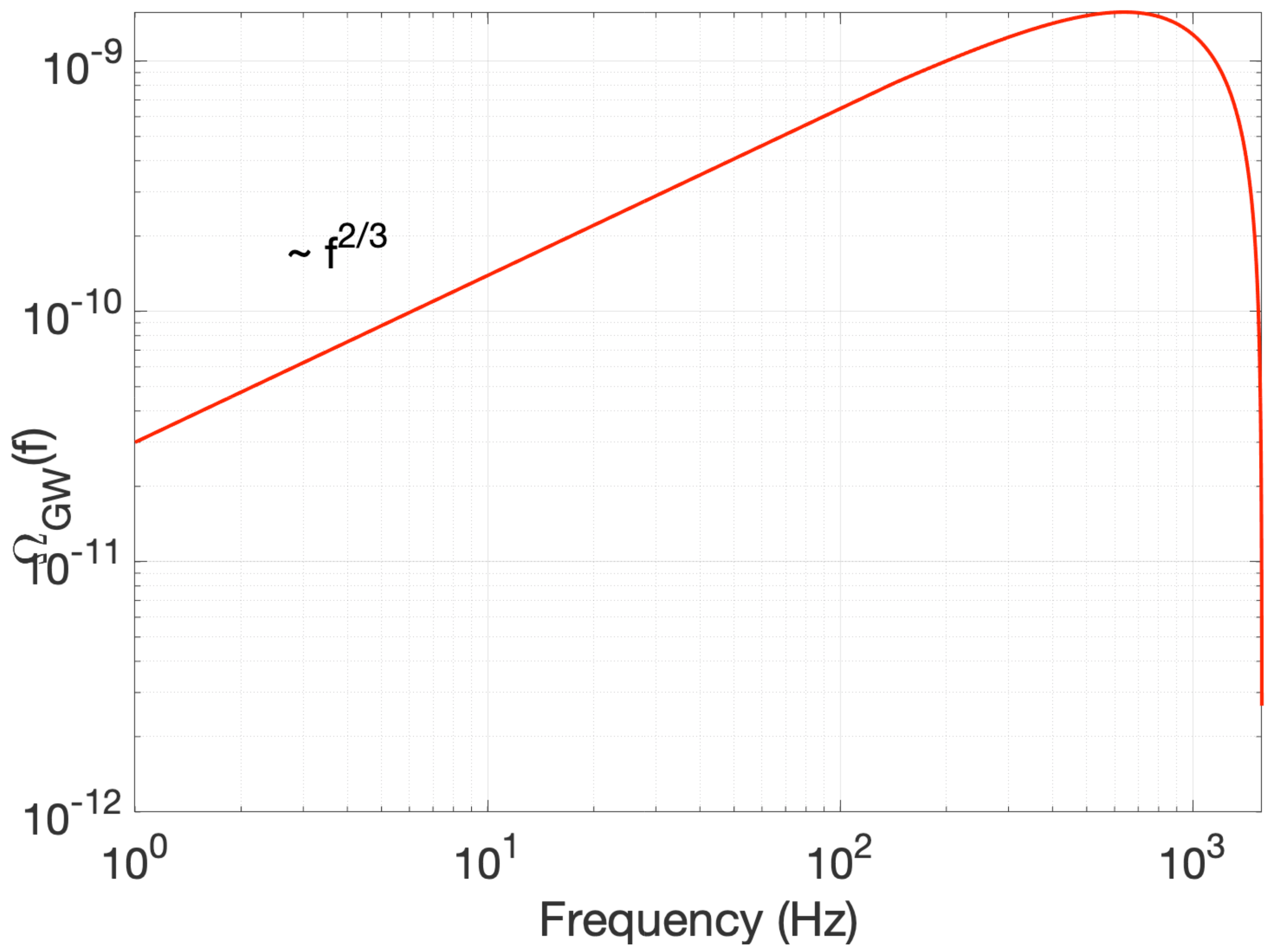
3. The Spectral Properties

Since the first studies on the gravitational-wave background were focusing on the primordial background, we historically characterize the GWB using the fractional energy density spectrum [67]:

$${\mathrm{\Omega }}_{GW}\left(f\right)=\frac{f}{{\rho }_c}\frac{d{\rho }_{GW}}{df}$$

(1)

where $d{\rho }_{\mathrm{GW}}$ is the energy density in the frequency interval f to $f+df$, ${\rho }_c=\frac{3H_0^2{c}^2}{8\pi G}$ is the critical energy density, and $H_0$ is the Hubble constant. The energy density parameter in GWs, that can be compared to other quantities used in cosmology such as the energy density parameters of matter, dark energy, relativistic particle or curvature, is:

$${\mathrm{\Omega }}_{\mathrm{GW}}=\int {\mathrm{\Omega }}_{\mathrm{GW}}\left(f\right)dlnf$$

(2)

Going back to the cosmological stochastic background formed by the overlap of many weak sources in the early Universe, it is assumed to be Gaussian because of the central limit theorem which says that the sum of a large number of independent variables converges to a normal distribution, whatever distribution the variables follow individually. It is also stationary in the sense that the normal distribution does not change with time. Figure 1 shows a time series of the GW strain amplitude of a Gaussian and stationary stochastic background: the amplitude $h\left(t\right)$ at any given time t follows a normal distribution centered in zero and with the same variance. It is also assumed to be isotropic by analogy with the Cosmic Microwave Background and unpolarized. Then it is completely characterized by the energy density spectrum as defined in Equation (2). However, when the background is non Gaussian, non stationary or non isotropic, which can be the case for astrophysical backgrounds, other quantities need to be introduced, as we will discuss later.

For a population of astrophysical sources from all over the Universe, the fractional energy density can be expressed as:

$${\mathrm{\Omega }}_{GW}\left(f\right)=\frac{f}{c{\rho }_c}{F}_{GW}\left(f\right)$$

(3)

The integrated flux in gravitational waves is given by the sum of all the individual contributions:

$$F_{GW}\left(f\right)={\int }_{\mathsf{\Theta }}p\left(\theta \right)d\theta {\int }_{z_{min}\left(\theta \right)}^{z_{max}\left(\theta \right)}dz\frac{dR}{dz}(\theta ,z){\mathrm{\Phi }}_{GW}(\theta ,z,f)$$

(4)

where $p\left(\theta \right)$ is the probability distribution of the source parameters $\theta$, $\mathsf{\Theta }$ represents the parameter space (for example the masses, the spins, the deformation of neutron stars), $\frac{dR}{dz}(\theta ,z)$ is the observed rate in the redshift interval $z-z+dz$, for sources with parameters $\theta$, and ${\mathrm{\Phi }}_{GW}\left(f\right)$ is the fluence at the observer frequency f from of a source with parameters $\theta$ at redshift z. The lower and upper limits of the integral $z_{min}\left(\theta \right)$ and $z_{max}\left(\theta \right)$ are the minimum and the maximum redshifts at which a source with parameters $\theta$ can be formed. They are related to the parameters $\theta$ through the minimal and maximal emission frequencies:

$$z_{\min }\left(f\right)=max(0,{\displaystyle \frac{f_{s;min}\left(\theta \right)}{f}}-1)$$

(5)

and

$$z_{\max }\left(f\right)=min(z_{max},{\displaystyle \frac{f_{s;max}\left(\theta \right)}{f}}-1)$$

(6)

where $f_{s;min}\left(\theta \right)$ and $f_{s;min}\left(\theta \right)$ are the minimal and the maximal emission frequency of the source. In the case of compact binary coalescences, they correspond to the initial at the birth of the compact binary system and the final frequency.

Replacing the fluence by the following expression:

$${\mathrm{\Phi }}_{GW}(\theta ,z,f)=\frac{1}{4\pi r{\left(z\right)}^2}\frac{d{E}_{GW}}{d{f}_s}(\theta ,f_s)$$

(7)

where $r\left(z\right)$ is the proper distance, $d{E}_{gw}/d{f}_s$ is the energy density emitted by a single source, $f_s=f(1+z)$ is frequency in the source frame, one obtains:

$$F_{GW}\left(f\right)={\int }_{\mathsf{\Theta }}p\left(\theta \right)d\theta {\int }_{z_{min}\left(\theta \right)}^{z_{max}\left(\theta \right)}dz{\displaystyle \frac{d{R}_z}{dz}}(\theta ,z)\frac{1}{4\pi r{\left(z\right)}^2}{\displaystyle \frac{d{E}_{GW}}{d{f}_s}}(\theta ,f_s)$$

(8)

The rate per interval of redshift is often calculated from the rate per comoving volume $R\left(z\right)$:

$${\displaystyle \frac{d{R}_z}{dz}}\left(z\right)={\displaystyle \frac{R\left(z\right)}{1+z}}{\displaystyle \frac{dV}{dz}}\left(z\right)$$

(9)

where the factor $1+z$ in the denominator converts $R\left(z\right)$ given in the source frame to the observer frame, and where the comoving volume element is:

$${\displaystyle \frac{dV}{dz}}\left(z\right)=4\pi r{\left(z\right)}^2{\displaystyle \frac{c}{H_{0}E\left(z\right)}}$$

(10)

For a flat $\mathsf{\Lambda }$CDM cosmology (neglecting the radiation term):

$$E_z\left(z\right)=\sqrt{{\mathrm{\Omega }}_M{(1+z)}^3+{\mathrm{\Omega }}_{\mathsf{\Lambda }}}$$

(11)

captures the dependence of the comoving volume on redshift (see for e.g., [68]) where ${\mathrm{\Omega }}_M$ is the energy density parameter of matter and ${\mathrm{\Omega }}_{\mathsf{\Lambda }}$ the energy density parameter of dark energy.

Combining the expressions above and after simplification we obtain the formula [46,48,52]:

$${\mathrm{\Omega }}_{GW}\left(f\right)={\displaystyle \frac{f}{{\rho }_c{H}_0}}{\int }_{\mathsf{\Theta }}p\left(\theta \right)d\theta {\int }_{z_{min}\left(\theta \right)}^{z_{max}\left(\theta \right)}dz{\displaystyle \frac{R(\theta ,z){\displaystyle \frac{d{E}_{gw}(\theta ,f_s)}{d{f}_s}}}{(1+z)E_z\left(z\right)}}$$

(12)

4. The Case of Compact Binary Mergers

The population of extra-galactic compact binaries formed by two black holes, two neutron stars or a neutron star and a black hole is the most interesting example of a GW background in the frequency band of terrestrial detectors for different reasons. First, we have started to observe the closest and the loudest mergers of such systems with second generation detectors LIGO and Virgo, and we have already obtained constraints about the rate and the distribution of masses or spins. Second, the waveform is well modelled and thus the shape of the fractional energy density spectrum. And finally we expect this background to dominate over all the other backgrounds and to be detected first. This background is also present in the space detector LISA at lower frequencies.

Compact binaries emit gravitational waves when they inspiral around each others and merge to produce a single neutron star or a black hole. In the frequency band of terrestrial detectors, we observe the very last moment of the inspiral phase, close to the merger, when the orbit has been circularized and we can assume there is no evolution of the redshift. In this case, the rate $R\left(z\right)$ corresponds to the merger rate and the spectral energy density spectrum of a single source $d{E}_{gw}/d{f}_s$, is obtained from the relation for circular orbit [39]:

$${\displaystyle \frac{1}{4\pi r^2}}{\displaystyle \frac{d{E}_{gw}}{d{f}_s}}\left(f_s\right)={\displaystyle \frac{\pi c^3}{2G}}{f}_s^2(H_{+}^2\left(f_s\right)+H_{\times }^2\left(f_s\right))$$

(13)

where $H_{+}\left(f_s\right)=A\left(f_s\right)(1+{cos}^2\iota )/2$ and $H_{\times }\left(f_s\right)=A\left(f_s\right)cos\iota$ are the Fourier amplitudes of the two polarization states, $\iota$ is the inclination angle, and r is the proper distance. Following recent papers e.g., [45,46,48], we can consider the inspiral phase only for BNSs and BHNSs and use the Newtonian waveforms up to the last stable orbit $f_{\mathrm{ISCO}}=\frac{c^3}{6^{3/2}G\pi M}$, $M=m_1+m_2$ being the total mass (i.e., the sum of the component masses $m_1$ and $m_2$ of the two compact objects), which gives:

$$A\left(f_s\right)=\sqrt{\frac{5}{24}}\frac{{\left(G{\mathcal{M}}_c\right)}^{5/6}}{{\pi }^{2/3}{c}^{3/2}}{\displaystyle \frac{1}{r}}{f}_s^{-7/6}$$

(14)

where ${\mathcal{M}}_c={\left(m_1{m}_2\right)}^{3/5}/{(m_1+m_2)}^{1/5}$ is the chirp mass. Replacing in Equation (13), we obtain ($N,C$ stands for Newtonian and circular):

$${\displaystyle \frac{d{E}_{gw}^{N,C}}{d{f}_s}}\left(f_s\right)={\displaystyle \frac{5{\left(G\pi \right)}^{2/3}{\mathcal{M}}_c^{5/3}{F}_{\iota }}{12}}{f}_s^{-1/3}$$

(15)

where $F_{\iota }={(1+{cos}^2\iota )}^2/4+{cos}^2\iota$.

For BBHs, we consider also the merger and ringdown and we use the phenomenological waveform $A\left(f\right)$ of [69], which gives ($P,C$ stands for phenomenological and circular):

$$\frac{d{E}_{gw}^{P,C}}{d{f}_s}\left(f_s\right)=\frac{d{E}_{gw}^{N,C}}{d{f}_s}\left(f_s\right)g\left(f_s\right)$$

(16)

where

$$g\left(f_s\right)=\left\{\begin{array}{cc}{(1+\sum _{i=2}^3{\alpha }_i{\nu }^i)}^2\hfill & \mathrm{if}{f}_s<f_1\hfill \\ f_s{w}_m{(1+\sum _{i=1}^2{ϵ}_i{\nu }^i)}^2\hfill & \mathrm{if}{f}_1\le f_s<f_2\hfill \\ f_s^{1/3}{w}_r{\mathcal{L}}^2(f_s,f_2,\sigma )\hfill & \mathrm{if}{f}_2\le f_s<f_3\hfill \end{array}\right.,$$

(17)

In this expression, $f_1$, $f_2$ and $f_3$ are the frequencies at the end of the inspiral, merger and ringdown phases, $\nu ={\left(\pi Mf\right)}^{1/3}$ and $\mathcal{L}(f,f_{ring},\sigma )$ is the Lorentz function centered at $f_2$ and with width $\sigma$, $w_m$ and $w_r$ are normalization constants ensuring the continuity between the three phases.

The other various constants are defined as

$$\begin{array}{c}{ϵ}_1=1.4547\chi -1.8897,\hfill \\ {ϵ}_2=-1.8153\chi +1.6557,\hfill \\ {\alpha }_2=-323/224+451\eta /168,\hfill \\ {\alpha }_3=(27/8-11\eta /6)\chi ,\hfill \end{array}$$

(18)

where $\eta =m_1{m}_2/{(m_1+m_2)}^2$ is the symmetric mass ratio and $\chi ={\displaystyle \frac{(m_1{\overrightarrow{\chi }}_1+m_2{\overrightarrow{\chi }}_2)}{M}}·{\displaystyle \frac{\overrightarrow{L}}{L}}$ is called the effective spin, and is a weighted combination of the projections of the individual spins ${\overrightarrow{\chi }}_1$ and ${\overrightarrow{\chi }}_2$ on the angular momentum $\overrightarrow{L}$.

The frequencies at the end of the different phases and $\sigma$ (${\mu }_k=f_1,f_2,\sigma ,f_3$) are calculated using Equation (2) of [69]:

$${\displaystyle \frac{G\pi M}{c^3}}{\mu }_k={\mu }_k^0+\sum _{i=1}^3\sum _{j=0}^N{x}_k^{ij}{\eta }^i{\chi }^j$$

(19)

where $N=min(3-i,2)$ and where the coefficients ${\mu }_k^0$ and $x_k^{ij}$ are given in Table I of [69].

5. Examples of Models for Compact Binary Mergers

As seen in the previous section, the calculation of the fractional energy density spectrum requires a model for the merger rate and for the distribution of the parameters $\theta$. The later can be inferred from theoretical predictions, population synthesis or since recently from constraints obtained with the individual detections by the collaboration LIGO–Virgo–Kagra.

5.1. Simple Model

We will look first at a very simple model of BNSs whose aim is to understand the different parts of the spectrum. We assume that all the systems have the same mass and that $m_1=m_2$. In this case the chirp mass is related to the total mass as ${\mathcal{M}}_c=M/4^{3/5}$. Furthermore, we assume a constant merger rate $R\left(z\right)=r_0$ in the range $z=0–10$ and null after.

In this scenario, the fractional energy density of Equation (12) can be expressed as:

$${\mathrm{\Omega }}_{GW}\left(f\right)={\displaystyle \frac{8{\pi }^{5/3}}{9}}{\displaystyle \frac{G^{5/3}}{H_0^3{c}^2}}{r}_0{\mathcal{M}}_c^{5/3}{I}_z\left(f\right)f^{2/3}$$

(20)

where we have averaged $F_{\iota }$ over a uniform distribution of $cos\left(\iota \right)$ which gives $F_{\iota }^{iso}=4/5$. In the expression above,

$$I_z\left(f\right)={\int }_0^{z_{\mathrm{up}}\left(f\right)}{\displaystyle \frac{dz}{{(1+z)}^{4/3}{E}_z\left(z\right)}},$$

(21)

where

$$z_{\mathrm{up}}\left(f\right)=min(z_{max},{\displaystyle \frac{f_{ISCO}}{f}}-1)$$

(22)

is the redshift after which the emitted frequency $f_s=f(1+z)$ becomes larger than $f_{ICSO}$.

Figure 2, Figure 3 and Figure 4 show the evolution of $z_{up}\left(f\right)$, $I_z\left(f\right)$ and $f^{2/3}{I}_z\left(f\right)$ as a function of the frequency f for component masses $m_1=m_2=1.4$ M${}_{\odot }$. The spectrum for this simple model is shown in Figure 5. At $z_{max}=10$, the frequency at the last stable orbit is observed at $f=143$ Hz for component masses $m_1=m_2=1.4$ M${}_{\odot }$, meaning that up to 143 Hz, all the sources contributes to the fractional energy density, which gives an evolution as ${\mathrm{\Omega }}_{gw}\left(f\right)$∼$f^{2/3}$, with an amplitude that depends on $r_0{\mathcal{M}}_c^{5/3}{I}_{max}$ where $I_{max}={\int }_0^{10}{\displaystyle \frac{dz}{{(1+z)}^{4/3}{E}_z\left(z\right)}}=0.93$. After this frequency, sources leave the band, starting with the more distant ones, reducing the factor $I_z\left(f\right)$ and at the same time the slope of ${\mathrm{\Omega }}_{GW}$ that deviates slowly from ${\mathrm{\Omega }}_{GW}$∼$f^{2/3}$ until the spectrum reaches a maximum at about 650 Hz; it then drops steeply to finally become zero at $f=f_{ISCO}$ where $I_z\left(f_{ISCO}\right)=0$ and only local sources at $z=0$ remain.

5.2. Model from GW Catalogs

In the case of isolated systems (other formation channels include dynamical captures in dense environments and primordial binary black holes) whose progenitors are massive stars binaries that have remained bound after the formation of the two compact objects, the merger rate $R(z,\theta )$ can be derived from the formation rate, although shifted by a delay $t_d$ between the formation of the massive binary at a redshift $z_f$ and the merger of the compact objects at z. This delay is the sum of the evolution time $t_b$, between the birth of the massive stars and the formation of the compact object, and the coalescence time $t_m$.

The time delay which connects $z_f$ to z is also the difference in cosmological lookback times:

$$t_d=t_c\left(z_f\right)-t_c\left(z\right)$$

(23)

where

$$t_c\left(z\right)={\int }_0^z\frac{d{z}^{\prime }}{H_0(1+z^{\prime })E_z\left(z^{\prime }\right)}d{z}^{\prime }$$

(24)

A model that has been often used in the literature assumes that the cosmic merger rate is an average over the intrinsic parameters $\theta$ and results from the convolution product:

$$R\left(z\right)=\int R_f\left(z_f(z,t_d)\right)P_{t_d}\left(t_d\right)d{t}_d$$

(25)

between the formation rate

$$R_f\left(z_f\right)=r_0\frac{SFR\left(z_f\right)}{SFR\left(0\right)}$$

(26)

where $SFR$ is the cosmic star formation rate in M${}_{\odot }$ yr${}^{-1}$Gpc${}^3$ and $r_0$ is the local rate in yr${}^{-1}$Gpc${}^{-3}$ that can be inferred from observations. The probability distribution of the delay is assumed to be of the form:

$$P_{t_d}\left(t_d\right)\sim \frac{1}{t_d}$$

(27)

with a maximum delay equal to the Hubble time and a minimal delay that depends on the type of binaries, 20 Myr for BNSs and 50 Myr for BHNSs and BBHs. The short mergers rate are predicted from population synthesis of isolated binaries such as StarTrack [71]. It does not apply to dynamical binaries or primordial black holes for which different models should be used.

Combining all the equations above we obtain:

$${\mathrm{\Omega }}_{GW}\left(f\right)={\displaystyle \frac{8{\pi }^{5/3}}{9}}{\displaystyle \frac{G^{5/3}}{H_0^3{c}^2}}\int d\theta p\left(\theta \right){\mathcal{M}}_c^{5/3}{I}_z(\theta ,f)f^{2/3}$$

(28)

where

$$I_z\left(f\right)={\int }_0^{z_{\mathrm{up}}(\theta ,f)}{\displaystyle \frac{R\left(z\right)}{{(1+z)}^{4/3}{E}_z\left(z\right)}}dz$$

(29)

with $\theta =m_1,m_2$ for BNSs and $\theta =m_1,m_2,{\overrightarrow{s}}_1,{\overrightarrow{s}}_2$ for BBHs. Here we have again averaged over an isotropic distribution of the inclination angle.

The first part of the third observation run O3a by the LIGO-Virgo collaboration gives a constraint on the local rate of $r_0={320}_{-240}^{+490}$ Gpc${}^{-3}$yr${}^{-1}$ for BNSs and $r_0={19}_{-8}^{+18}$ Gpc${}^{-3}$yr${}^{-1}$ for BBHs. At that time, no BHNSs had been observed and only an upper limit was reported. Figure 6 shows the average merger rate for BNSs (blue) and BBHs (red) derived from the equations above using the star formation rate of [70] (Vangioni et al.), as in [46,48].

On the other hand, the O3a catalog favors a uniform distribution of the component masses, between $1–3$ M${}_{\odot }$ for BNSs and a broken power law for BBHs. Ref. [72] assumed a sharp low-mass cut-off in the BBH mass spectrum, corresponding to ${\delta }_m=0$ in Equation (B6) of [73]), which gives:

$$p\left(m_1\right)\propto \left\{\begin{array}{cc}{m}_1^{{\alpha }_1}\hfill & \mathrm{if}{m}_{min}<m_1<m_b\hfill \\ m_1^{{\alpha }_2}\hfill & \mathrm{if}{m}_b<m_1<m_{max}\hfill \end{array}\right.$$

(30)

with ${\alpha }_1=-1.74$, ${\alpha }_2=-6.27$, $m_{min}=5.64$ M${}_{\odot }$, $m_{max}=76.6$ M${}_{\odot }$ and $m_b=38.59$ M${}_{\odot }$, for the largest component mass and

$$p\left(q\right)\propto q^{{\beta }_q}$$

(31)

with ${\beta }_q=1.37$ for the mass ratio $q=m_2/m_1$ where $m_2<m_1$.

Figure 7 shows the fractional energy density spectrum for the population of BNSs (blue), BBHs (red) and the total (black). The filled areas corresponds to the error on the local rate and do not integrate all the uncertainty on the models. The average values of ${\mathrm{\Omega }}_{GW}$ at 25 Hz are about $3\times {10}^{-10}$ for BBHs and $2\times {10}^{-10}$ for BNS. There is a slight difference for BBHs compared to the results in [72] ($5\times {10}^{-10}$) due to the fact that for simplicity we have used the median values rather than included the uncertainty on the BBH mass distribution parameters. In addition, we have neglected the metallicity cutoff that can apply to larger mass BBHs and that is not well understood (see [46]) (after we have written this section, the LIGO–Virgo–Kagra collaboration released a new catalog including observations during the second half of the O3 observational run [74] and updated the predictions for the background from binaries [75]. They find a total energy density spectrum including BH-NS of the ${\mathrm{\Omega }}_{GW}\left(25\mathrm{Hz}\right)=6.9_{-2.0}^{3.5}\times {10}^{-10}$).

In order to quantify the effect of changing the star formation history or the delay time, Refs. [43,46] have explored variations to the fiducial model, and found differences within a factor of two i.e., smaller than the error on the rate. In a paper that followed the first BBH detection (GW150914), Ref. [47] calculated the fractional energy density spectrum of BBHs for different redshift dependant mass distributions derived from black holes formation channels in which the cosmic chemical evolution simultaneously matches observations of the cosmic star formation rate, optical depth to reionization and metallicity of the interstellar medium. Their results are in agreement with the predictions of [46] and show the importance of considering a mass distribution.

5.3. Model from Simulations

Using an analytical formula to calculate ${\mathrm{\Omega }}_{GW}$ is very convenient for simple models like the ones discussed above, but can become quite complicated and computationally expensive with more parameters, correlations between them or evolution of the parameter with redshift. A better strategy in this case is to use Monte Carlo simulations to generate a population of sources with the required distribution in the parameter space and then calculate ${\omega }_{GW}$ as the sum of the contribution from each source. In order to reproduce the result of the previous section, one could proceed as follow for each event k:

• The time interval from the previous event ${\tau }^k$ is drawn from an exponential probability distribution $P\left(\tau \right)=exp(-\tau /\lambda )$, assuming a Poisson process. The average waiting time is computed from the inverse of the total rate in the observer frame, integrated over the volume of the Universe.

  $$\lambda ={\left({\int }_0^{10}dz{\displaystyle \frac{dR}{dz}}\left(z\right)\right)}^{-1}$$

  (32)
• The redshift $z^k$ is drawn from a probability distribution $p\left(z\right)$ constructed by normalizing in the interval $0–10$ the coalescence rate ${\displaystyle \frac{dR}{dz}}\left(z\right)$ (9).
• The cosine of the inclination angle, $cos{\iota }^k$, is drawn from a uniform distribution in the range of [−1, 1]. In addition, each event is given a sky position (equatorial declination ${\delta }^k$ and right ascension $r{a}^k$) and a polarization angle, ${\psi }^k$. In the simple models we are considering here we assume isotropic distributions.
• the component masses $m_1^k$ and $m_2^k$ are drawn from the mass distributions given in the previous sections and the spins of BHs $s_1^k$ and $s_2^k$ are taken equal to zero for this model but can be drawn too from a distribution.
• for each observed frequency f, we can then calculate the fluence of the source k:

  $${\mathrm{\Phi }}_{GW}^k\left(f\right)=\frac{1}{4\pi r^2\left(z^k\right)}\frac{d{E}_{gw}}{df}({\theta }^k,f_s)$$

  (33)
  It is convenient to write this equation in term of the observed quantities: luminosity distance $d_L=r(1+z)$, observed frequency $f=f_s=(1+z)$ and redshifted masses $m_{i,z}=m_i(1+z)$:

  $${\mathrm{\Phi }}_{GW}^k\left(f\right)=\frac{1}{4\pi d_L^2\left(z^k\right)}\frac{d{E}_{gw}}{df}({\theta }^k,f)$$

  (34)

Finally, the energy flux in is calculated by adding together all the contributions:

$$F_{GW}\left(f\right)=\frac{1}{T}\sum _{k=1}^N{f}_{GW}^k\left(f\right)$$

(35)

and calculate the energy density spectrum ${\mathrm{\Omega }}_{GW}$ from (3).

The Monte Carlo procedure can be used to calculate the fractional energy density spectrum from any probability distributions of the parameters but also from lists of sources whose parameters are the end products of sophisticated population synthesis and binary evolution codes, a case which could not be done analytically. In a recent paper, ref. [49] have used simulated populations produced by the code StarTrack to calculate the background of all types of binaries, including population III stars and binaries that do not merge in a Hubble time. The code follows the formation and evolution of massive stars as well as the evolution of the orbital parameters for given redshift and metallicity and provides the evolution time to form the system of compact objects, the merger time, the masses of the compact objects, the initial separation and eccentricity and the spins. With these information, it is possible to account for the correlations between the parameters as well as the eccentricity and redshift evolution at low frequencies, when the sources evolve slowly. However, it was shown that even in the LISA band the impact of eccentricity is negligible.

In a second paper, Ref. [50] have used simulated populations produced by the code MOBSE to calculate the background of all types of binaries, for both the isolated formation channel considered until now and the dynamical channel. The dynamical channel can boost the background by a factor a bit less than two, depending on what fraction of the total population of CBCs, this channel represents. The results of these two studies are compatible with the ones derived in the previous section, and indicates a value of ${\mathrm{\Omega }}_{GW}\left(25\mathrm{Hz}\right)$∼${10}^{-9}$ for the contribution of all the types of CBCs. Notice that the background from population III as predicted by [49] with the StarTrack data is one order of magnitude below but can have an impact in third generation detectors as we will see later.

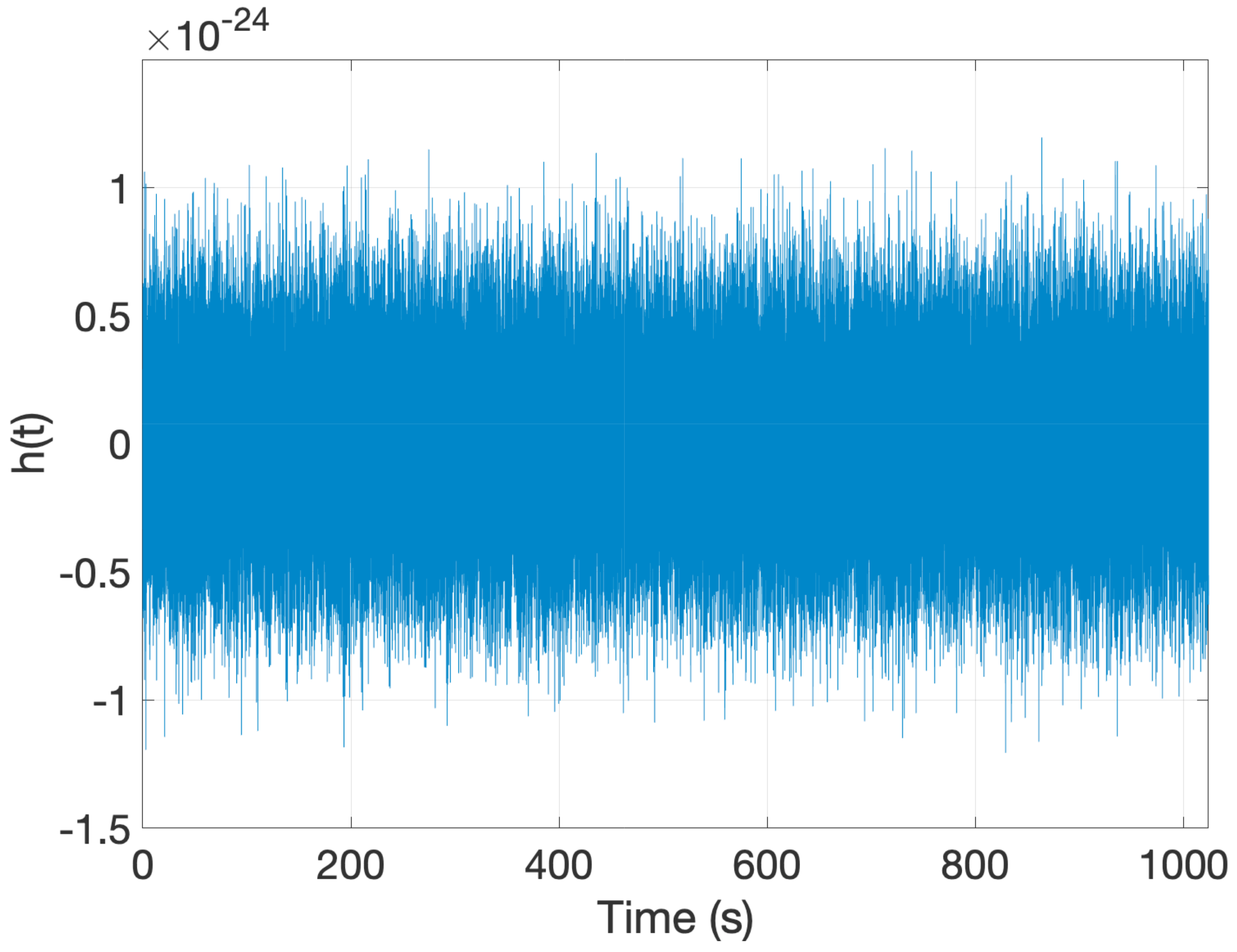
6. Properties in the Time Domain: Continuity

The backgrounds from BNS and BBH population have similar fractional energy density spectrum (see Figure 7) but there statistical properties can be very different and so their behavior in the time domain.

Figure 8 shows a simulated time series of the GW strain amplitude $h\left(t\right)$, in a detector like LIGO, Virgo, Kagra or the future LIGO India with a lower frequency of 10 Hz, for both the BNS and BBH backgrounds whose fractional energy density spectra corresponds to the median plots in Figure 7. The BNS population creates a continuous background consisting of a superposition of overlapping sources, while the BBH population create a highly non-continuous, non-stationary background of individual events well separated on time often referred to as popcorn.

Whether a background is continuous or not can be quantified by the so called duty cycle (see for instance [76]),

$$\Delta ={\int }_0^{z_{max}}\tau ({\mathcal{M}}_c,f_L)(1+z){\displaystyle \frac{dR}{dz}}\left(z\right)dz$$

(36)

which is the average number of events that overlap at any given moment and is defined as the ratio, of the typical duration of a single event in the detector, to the average time interval between successive events. The factor ($1+z$) converts the duration in the source frame to the detector frame.

The duration in the source frame is given at leading order by

$$\tau ({\mathcal{M}}_c,f_L)={\displaystyle \frac{5c^5}{256{\pi }^{8/3}{G}^{5/3}}}{\mathcal{M}}_c^{-5/3}{f}_L^{-8/3},$$

(37)

where $f_L$ is the lower frequency bound of the detector, assumed to be much smaller than the frequency at the time of the merger. The signal duration depends very strongly on both the chirp mass and the lower frequency bound. In particular, more massive binaries such as BBHs have shorter duration and signals measured by instruments with low $f_L$ have longer duration:

• For a system of BNS with component masses of 1.4 M${}_{\odot }$ (a chirp mass ${\mathcal{M}}_c=1.2$ M${}_{\odot }$), the duration is 1000 s in 2G detectors with $f_L=10$ Hz and 6351 s in 3G detectors with $f_L=5$ Hz or 5.4 days if we can push the lower frequency band down to $f_L=1$ Hz.
• For a system of two black holes with component masses of 15 M${}_{\odot }$ (a chirp mass ${\mathcal{M}}_c=13$ M${}_{\odot }$), the duration is 19.4 s in 2G detectors with $f_L=10$ Hz and 123 s in 3G detectors with $f_L=5$ Hz or 2.5 h if we can push the lower frequency band down to $f_L=1$ Hz.

For the case shown in Figure 7, BNSs are more frequent than BBHs (the average waiting time between two BNSs is 63 s and between two BBHs 1242 s) and stay longer in band than BBHs (the average BNS duration is 164 s for BNSs and 10.5 s for BBHs), resulting in a continuous background for BNSs with a duty cycle of $\Delta =2.6$ and events separated in times for BBHs with $\Delta =8.5\times {10}^{-3}$.

7. Residual Background

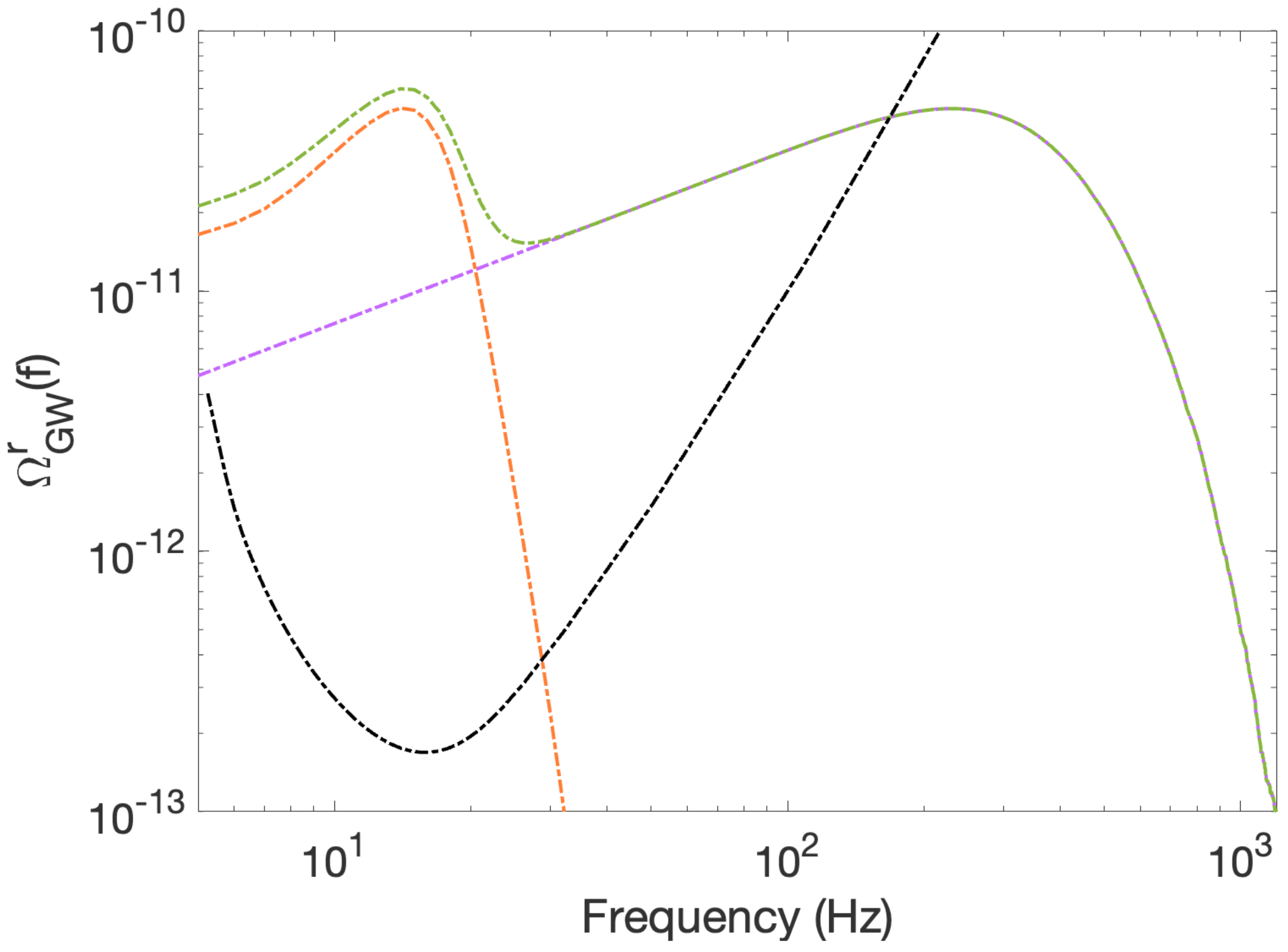
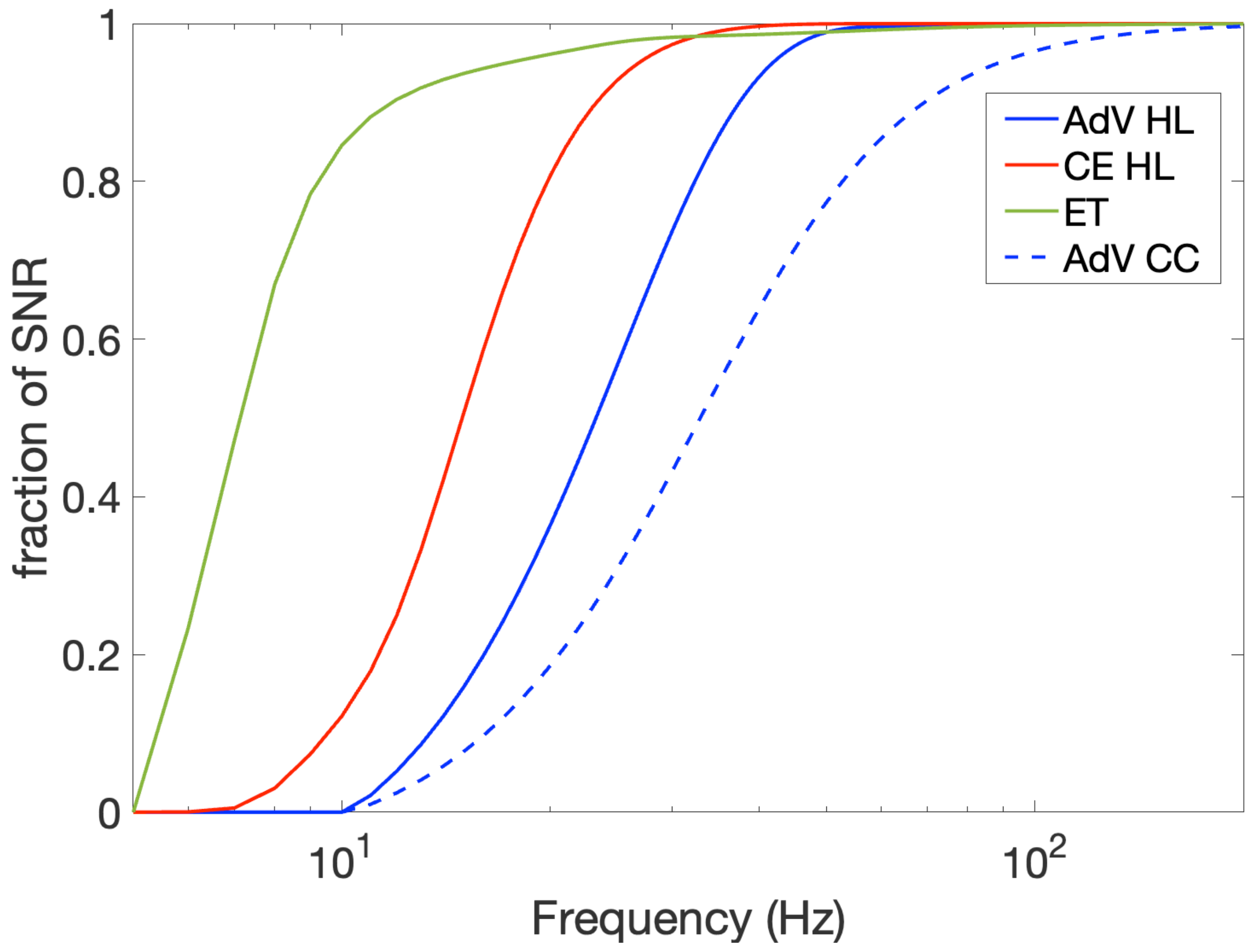
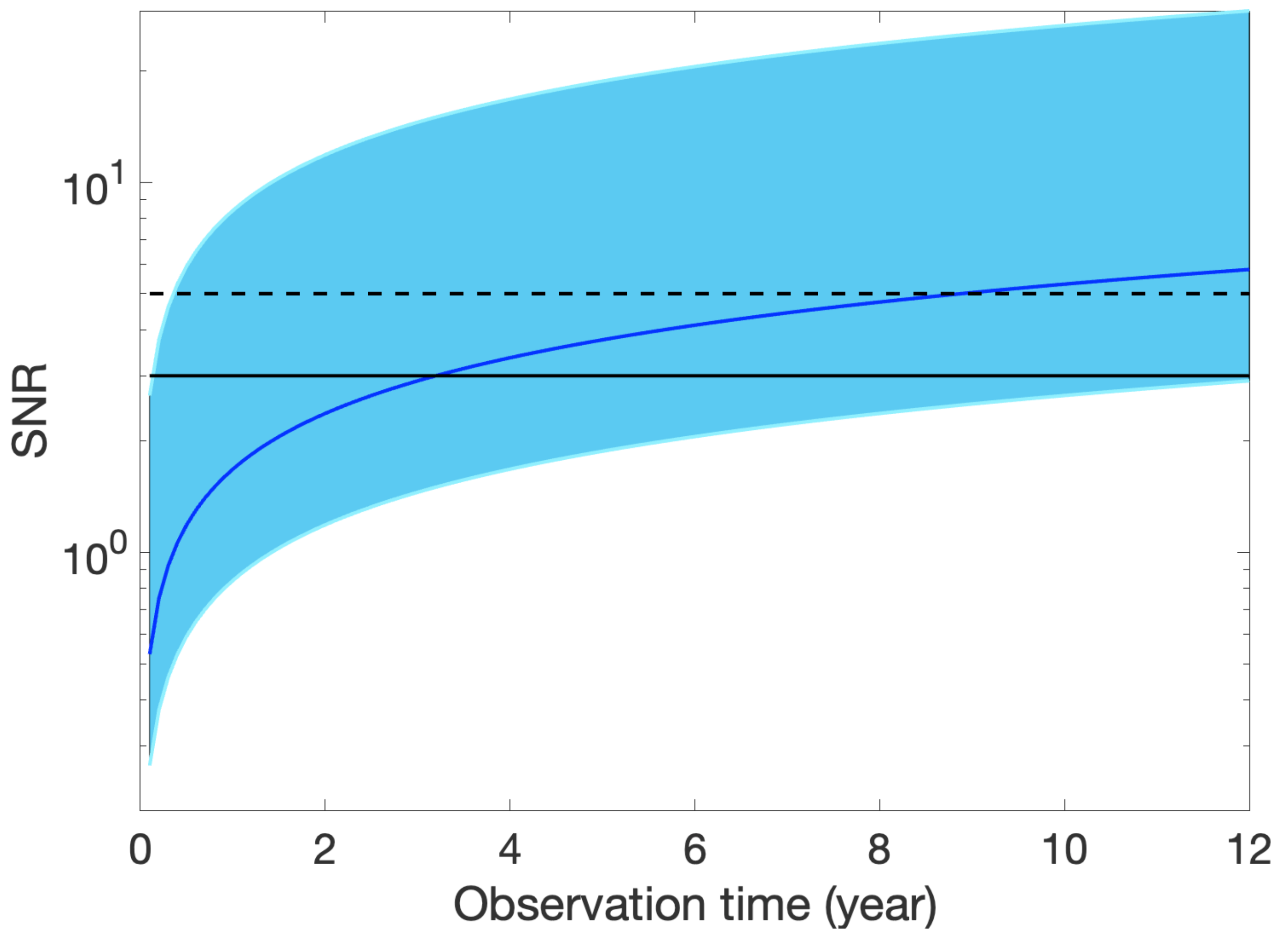
Even for BNSs and the largest predicted rate, the number of overlapping sources is not large enough to create a confusion background in the frequency band of ground based detectors. Actually, when whitened with the sensitivity of the detectors, the GW strain time series look like a collection of well separated events, and those whose signal-to-noise ratio is above the detection threshold ${\rho }_T$ can be detected individually. Here, we follow previous work and assume ${\rho }_T=12$ [49,50].

For a network of N terrestrial detectors the coherent signal-to-noise ratio (SNR), assuming optimal matched filtering and uncorrelated Gaussian noise in the detectors, is given by:

$$\rho ={[\sum _{i=1}^{N}4{\int }_{f_{i,min}}^{f_{i,max}}\frac{{\left|F_{+,i}(t,f,ra,\delta ,\psi )H_{+}\left(f\right)+F_{\times ,i}(t,f,ra,\delta ,\psi )H_{\times }\left(f\right)\right|}^2}{P_i\left(f\right)}df]}^{1/2}$$

(38)

where the index i refers to the detectors, $f_{i,min}$ and $f_{i,max}$ are the low and high frequency bounds of their sensitivity band, $F_{+,i}$ and $F_{\times ,i}$ are the antenna response functions to the + and × polarizations, that depends on the sky position and polarization of the source, and $P_i\left(f\right)$ is the one-sided noise power spectral density of the ith detector.

Figure 9 shows detection efficiency ${\epsilon }^D\left(z\right)$ integrated over sky positions, polarization and inclination angle for the network of second generation detectors LIGO Hanford (H), LIGO Livingston (L) and Virgo (V), for a neutron star binary of equal component masses 1.4 M${}_{\odot }$ (blue) and for a black hole binary of equal component masses 15 M${}_{\odot }$ (red); we assume spins of zero for BHs. At $z=0$, all the sources can be detected and the efficiency is equal to one, then it decreases to reach zero at the horizon distance where only a source positioned and oriented optimally is detected. Because of the selection effect on the population of detected sources, the distribution of the orientation angle, for the residual background, is not isotropic. Figure 10 shows the evolution of the average value of the orientation parameter $<F_{\iota }>$ as a function of the redshift, for the same examples as in Figure 9.

Using these two functions, Equation (28) can be written for the residual background as:

$${\mathrm{\Omega }}_{GW}^{r,D}\left(f\right)={\displaystyle \frac{8{\pi }^{5/3}}{9}}{\displaystyle \frac{G^{5/3}}{H_0^3{c}^2}}{\int }_{\mathsf{\Theta }}d\theta p\left(\theta \right){\mathcal{M}}_c^{5/3}{I}_z^{r,D}(\theta ,f)f^{2/3}$$

(39)

with

$$I_z^{r,D}(\theta ,f)={\int }_0^{z_{\mathrm{up}}(\theta ,f)}{\displaystyle \frac{(1-{\epsilon }^D(\theta ,z))\overline{F_{\iota }^D}(\theta ,z)}{{(1+z)}^{4/3}{E}_z\left(z\right)}}$$

(40)

where $\overline{F_{\iota }^D}\left(z\right)={\displaystyle \frac{<F_{\iota }^D(\theta ,z)>}{F_{\iota }^{iso}}}$ with $F_{\iota }^{iso}=4/5$.

Figure 11 shows the residual backgrounds for the population of BNSs (blue) and BBHs (red) for the network of second generation detectors HLV (continuous line), and for two third generation detector networks, Einstein Telescope (dashed line) and ET with two Cosmic Explorers (dot-dashed line). The black curves are the Power Integrated (PI) curves that indicate the sensitivity of the three networks of detector to a stochastic background. As described in [77], a power-law stochastic background that is tangent to a PI curve is detectable with a signal-to-noise-ratio of 2 after an effective integration time of 1 year (two years of real data if we assume a duty cycle of 50%).

The background can be decreased down to about two orders of magnitudes with 3G detectors for BNSs and four orders of magnitude for BBHs. The figure shows the best possible scenario where we are able to measure the exact parameters of the detected sources and subtract perfectly the waveform [61]. In practice, there is an extra residual due to the error we make on measuring the parameters and on the waveform model. Ref. [62] studied the effect of the uncertainties on the recovered parameters and found that for BBHs they dominate the residual background when for BNSs they are negligible compared to the residual due to undetected sources.

Using models from StarTrack, Ref. [49] calculated the residual for both population I/II and population III CBCs and found that the population III at large redshift, that was masked below the population I/II in 2G detectors could appear as a bump at low frequencies in the residual of 3G detectors. The shape of the spectrum would then deviate from the expected power law ${\mathrm{\Omega }}_{GW}\left(f\right)$∼$f^{2/3}$, providing evidence for the existence of this population. Figure 12 reproduces the results of [49] for the StarTrack model FS1 for population III (in orange) along with the sum of the BNS and BBH contributions of Figure 11 (purple). The total of the two curves is indicated in green, where we see the bump from population III CBCs below 30 Hz.

8. Detectability

The signal at the output of a detector contains both the instrumental noise and the gravitational-wave signal:

$$s_i=h_i+n_i$$

(41)

where $h_i$

$$h_i=h_{+,i}{F}_{+,i}+h_{\times ,i}{F}_{\times ,i}$$

(42)

The strategy to search for a stochastic background, which could be confounded with the intrinsic instrumental noise, is to cross-correlate measurements of two (or multiple) detectors. In theory, it permits to eliminate the noise that is assumed to be uncorrelated between the two detectors i and j and with the signal:

$$<s_i{s}_j>=<h_i{h}_j>+\underset{=0}{\underbrace{<n_i{n}_j>}}+\underset{=0}{\underbrace{<h_i{n}_j>}}+\underset{=0}{\underbrace{<n_i{h}_j>}}$$

(43)

In practice, environmental correlated noise may remain such as seismic or magnetic noise [78,79,80].

It is convenient to work in the frequency domain and write the cross-correlation product as:

$$Y=\int \widetilde{s_i}\left(f\right)\tilde{Q}\left(f\right)\widetilde{s_j}\left(f\right)df$$

(44)

where the tilde denote a Fourier transform and where $\tilde{Q}$ is an optimal filter that depends on the noise power spectral densities in the two detectors $P_i$ and $P_j$ and on the fractional energy density spectrum ${\mathrm{\Omega }}_{GW}$:

$$\tilde{Q}\left(f\right)=\lambda {\displaystyle \frac{{\gamma }_{ij}^{iso}\left(f\right){\mathrm{\Omega }}_{ij}\left(f\right)}{P_i\left(f\right)P_j\left(f\right)}}$$

(45)

In this equation, $\lambda$ is a normalisation constant and

$${\gamma }_{ij}^{iso}\left(f\right)=\frac{5}{8\pi }\sum _{A=+,\times }\int e^{i2\pi f\widehat{\mathrm{\Omega }}\Delta t}{F}_i^A\left(\widehat{\mathrm{\Omega }}\right)F_j^A\left(\widehat{\mathrm{\Omega }}\right)d\widehat{\mathrm{\Omega }}$$

(46)

is the isotropic overlap reduction function (ORF), normalized to take the value of 1 for co-aligned and coincident detectors. This function is the average over polarization and sky position of the overlap between the response tensors of the two detectors and characterizes the loss of sensitivity due to the relative orientations of the distance between them, that creates a delay $\Delta t$ between the arrival times at the two detectors for a wave coming from the direction $\widehat{\mathrm{\Omega }}$. Figure 13 shows examples of the ORF for pairs of detectors formed by LIGO Hanford (H), LIGO Livingston (L), Virgo (V), Kagra (K) and LIGO India (I). At a frequency $f=0$ Hz, the only effect is the non alignement of the detectors but the effect of the distance increases with the frequency and we observe an important drop of sensitivity after a few hundred Hz for all the pairs.

The average value of the cross correlation statistics $\mu$ gives an estimate of the signal and the variance $\sigma$ an estimate of the error. For a pair of detectors, we can write the optimal signal to noise ratio, SNR$={\displaystyle \frac{\mu }{\sigma }}$ as:

$${\mathrm{SNR}}_{ij}=\frac{3H_0^2}{10{\pi }^2}\sqrt{2T}{\left[{\int }_0^{\infty }df\frac{{\gamma }_{ij}^2\left(f\right){\mathrm{\Omega }}_{gw}^2\left(f\right)}{f^6{P}_i\left(f\right)P_j\left(f\right)}\right]}^{1/2},$$

(47)

where T is the observational time. For a network of n detectors, the combined SNR is obtained by calculating the quadratic sum:

$${\mathrm{SNR}}^2=\sum _{i=1}^n\sum _{j>i}{\mathrm{SNR}}_{ij}^2,$$

(48)

In the case of the background from CBCs, a natural template is ${\mathrm{\Omega }}_{GW}^T\left(f\right)={\mathrm{\Omega }}_{\mathrm{Ref}}{\left({\displaystyle \frac{f}{f_{\mathrm{Ref}}}}\right)}^{2/3}$, corresponding to the shape of the spectrum in the inspiral regime. In this case and as already discussed in [45], most of the SNR comes from a relatively small frequency interval that extends from a few Hz to <100 Hz (see Figure 14).

Figure 15 shows the evolution of the SNR with the effective observation time (the real time is twice the effective time for a duty cycle of 50%) for the network of advanced detectors at design sensitivity. We considered a background with ${\mathrm{\Omega }}_{GW}(25\mathrm{Hz}$) between $5\times {10}^{-10}–5\times {10}^{-9}$ taking into account the uncertainty from the most recent predictions. The background could be detected with a signal-to-noise ratio of 3 after a few months or a dozen years. The prediction from the latest LIGO–Virgo–Kagra catalog (${\mathrm{\Omega }}_{GW}\left(25\mathrm{Hz}\right)=5\times {10}^{-9}$) favors a observation time of 7 years when the models from the simulations StarTrack or MOBSE discussed in Section 5.3, with an average value of ${\mathrm{\Omega }}_{GW}\left(25\mathrm{Hz}\right)$∼${10}^{-9}$, predict a smaller observation time of 3 years.

With 3G detector the background will be observed with a large signal-to-noise ratio [49]. One may wonder whether it will still be interesting since the background has a good chance to be detected before. It is because we will observe mainly the residual from BNS sources and sources at higher redshift that were hidden below the contribution from closest sources in 2G detectors.

9. Possible Complications

9.1. Population III

If there is a population III that dominates in the residual of 3G detectors the shape of the spectrum will deviate from ${\mathrm{\Omega }}_{GW}\left(f\right)$∼$f^{2/3}$. Ref. [81] addresses this issue using a broken power law template to model the decrease of the spectrum after the peak at around 20 Hz.

9.2. Non Gaussianity

As discussed before, the background from CBC is expected to be non Gaussian in the frequency band of terrestrial detectors. The cross correlation statistic is optimal for stationary and Gaussian backgrounds; however, refs. [82,83] have shown that since the analysis is done in the frequency domain, what matters is the total number of sources within the integration time rather than whether they overlap in the time domain, and that standard cross-correlation statistics could detect the background from CBCs with no loss of sensitivity. More sensitive methods that take into account the non Gaussianity have been studied [84,85].

9.3. Anisotropy

Models predict that the GW background will present anisotropies due to the nature of spacetime along the line of sight, and for the astrophysical contribution, due to the local distribution of matter and the finitness of the number of sources. The past years a lot of work has been done to characterize anisotropies in particular in the background from CBCs [86,87,88,89,90,91,92,93,94,95].

They can be measured using a modified version of the isotropic cross-correlation statistics described in the previous section, where one relaxes the assumption of isotropy and generalizes to arbitrary angular distribution. In this case, the fractional energy density spectrum depends on the direction of the sky and takes the form:

$${\mathrm{\Omega }}_{GW}(f,\widehat{\mathrm{\Omega }})={\mathrm{\Omega }}_{GW}\left(f\right)P\left(\widehat{\mathrm{\Omega }}\right)$$

(49)

where ${\mathrm{\Omega }}_{GW}\left(f\right)$ is the averaged value (called the monopole) and $P\left(\widehat{\mathrm{\Omega }}\right)$ is the angular power distribution normalized to unity over the whole sky:

$${\int }_{S^2}P\left(\widehat{\mathrm{\Omega }}\right)d\widehat{\mathrm{\Omega }}=1$$

(50)

In order to probe anisotropies in the GW background, one can use a method similar to what is done in radio astronomy and that is called the GW radiometer [78,96,97]. GWs from different directions in the sky will arrive with different delays in two detectors and by correcting for these delays, it is possible to map $P\left(\widehat{\mathrm{\Omega }}\right)$ in a pixel or spherical harmonic basis. The overlap reduction function in the direction $\widehat{\mathrm{\Omega }}$ is the integrand of (46):

$${\gamma }_{ij}^{\widehat{\mathrm{\Omega }}}\left(f\right)=\frac{1}{2}\sum _{A=+,\times }{e}^{i2\pi f\widehat{\mathrm{\Omega }}\Delta t}{F}_i^A\left(\widehat{\mathrm{\Omega }}\right)F_j^A\left(\widehat{\mathrm{\Omega }}\right)$$

(51)

In addition, for 3G detectors, the residual background may not be isotropic because of the selection effect on the detected sources that are removed. Using simulated data, Ref. [98] calculated a that it could lead to systematic bias of about 1.25 if the isotropic version of the cross correlation statistics was used.

10. Summary and Conclusions

The GW background is expected to be detected in many frequency bands thanks to the tremendous efforts in improving the sensitivity of the detectors. Future CMB experiments on Earth (for instance CMB-S4 [99]) or in space (for instance LiteBird [54,100] ) will be able to reach values of the tensor to scalar ratio of the order of r∼${10}^{-4}$, i.e., a gain of 2–3 orders of magnitudes compared to the current upper limit of $r<0.032$ given by Planck 2018+BICEP+Keck [101]. This would translate into a sensitivity of $h_0^2{\mathrm{\Omega }}_{GW}$∼${10}^{-17}$ at f∼${10}^{-17}$ on the primordial background from inflation [54]. Pulsar timing arrays are constantly increasing the number of pulsars in their catalogs and NanoGrav may already be very close to confirm the detection of the background from SMBHB [57]. In the future, SKA [102] could reach a sensitivity of $h_0^2{\mathrm{\Omega }}_{GW}$∼${10}^{-13}$ at f∼${10}^{-9}–{10}^{-8}$ Hz [54]. In As for laser interferometers, both LISA in space and Einstein Telescope and Cosmic Explorer, planned to start collecting data around 2035, will reach a sensitivity of $h_0^2{\mathrm{\Omega }}_{GW}$∼${10}^{-13}$ [54], i.e., a gain of three orders of magnitude compared to the second generation of terrestrial detectors. Other proposals for space missions include BBO [103], the successor of LISA, the Japanese detector DECIGO [104], or the two chinese detectors TianQin [105] and Taiji [106], amoung others [54].

Combining the results of these experiments will provide precious complementary information on the very early stages of the Universe and its evolution before and after the beginning of stellar activity. In the frequency band of terrestrial detectors, we expect the background to be dominated by its astrophysical contribution and in particular the background formed by compact binary mergers. According to the predictions inferred from the constraints on the rate and the masses from sources detected individually at close distances, the detection of this background could be the next important milestone for GW astronomy and has received a lot of attention the past few years.

In this paper, we introduced the properties of the background from CBCs and show that it is non Gaussian and non stationary and then differs from what we expect for a stochastic background, for example of cosmological origin. Even if they look similar in the frequency domain, the background from BBHs appears in the time domain as a popcorn signal on the top of the continuous signal formed by BNSs, more frequent than BBHs and with longer duration. This can help distinguishing them in the future. At the moment we cannot either with the standard cross-correlation method separate the different formation channels but methods are being investigated that could lead to promising results. Another challenge will be to partially suppress the background by removing the sources detected individually in third generation detectors. This will provide the possibility to unveil the existence of a population III as well as observe other astrophysical contributions and maybe the background from cosmological origin.

References

1. Aasi, J.; Abbott, B.P.; Abbott, R.; Abbott, T.; Abernathy, M.R.; Ackley, K.; Adams, C.; Adams, T.; Addesso, P. Advanced LIGO. Class. Quant. Grav. 2015, 32, 074001. [Google Scholar] [CrossRef]
2. Acernese, F.A.; Agathos, M.; Agatsuma, K.; Aisa, D.; Allemandou, N.; Allocca, A.; Amarni, J.; Astone, P.; Balestri, G.; Ballardin, G. Advanced Virgo: A second-generation interferometric gravitational wave detector. Class. Quant. Grav. 2015, 32, 024001. [Google Scholar] [CrossRef] [Green Version]
3. Aso, Y.; Michimura, Y.; Somiya, K.; Ando, M.; Miyakawa, O.; Sekiguchi, T.; Tatsumi, D.; Yamamoto, H. Interferometer design of the KAGRA gravitational wave detector. Phys. Rev. 2013, D88, 043007. [Google Scholar] [CrossRef] [Green Version]
4. Grishchuk, L.P. Amplification of gravitational waves in an isotropic universe. Sov. J. Exp. Theor. Phys. 1975, 40, 409. [Google Scholar]
5. Grishchuk, L.P. Primordial gravitons and possibility of their observation. Sov. J. Exp. Theor. Phys. Lett. 1976, 23, 293. [Google Scholar]
6. Starobinskiǐ, A.A. Spectrum of relict gravitational radiation and the early state of the universe. Sov. J. Exp. Theor. Phys. Lett. 1979, 30, 682. [Google Scholar]
7. Bar-Kana, R. Limits on direct detection of gravitational waves. Phys. Rev. D 1994, 50, 1157–1160. [Google Scholar] [CrossRef] [Green Version]
8. Turner, M.S. Detectability of inflation-produced gravitational waves. Phys. Rev. D 1997, 55, R435–R439. [Google Scholar] [CrossRef] [Green Version]
9. Caprini, C.; Figueroa, D.G. Cosmological backgrounds of gravitational waves. Class. Quantum Gravity 2018, 35, 163001. [Google Scholar] [CrossRef] [Green Version]
10. Gasperini, M.; Veneziano, G. Pre-big-bang in string cosmology. Astropart. Phys. 1993, 1, 317–339. [Google Scholar] [CrossRef] [Green Version]
11. Gasperini, M.; Veneziano, G. The pre-big bang scenario in string cosmology. Phys. Rep. 2003, 373, 1–212. [Google Scholar] [CrossRef] [Green Version]
12. Mandic, V.; Buonanno, A. Accessibility of the pre-big-bang models to LIGO. Phys. Rev. D 2006, 73, 063008. [Google Scholar] [CrossRef] [Green Version]
13. Brustein, R.; Gasperini, M.; Giovannini, M.; Veneziano, G. Relic gravitational waves from string cosmology. Phys. Lett. B 1995, 361, 45–51. [Google Scholar] [CrossRef] [Green Version]
14. Buonanno, A.; Maggiore, M.; Ungarelli, C. Spectrum of relic gravitational waves in string cosmology. Phys. Rev. D 1997, 55, 3330–3336. [Google Scholar] [CrossRef] [Green Version]
15. Caprini, C.; Durrer, R.; Servant, G. Gravitational wave generation from bubble collisions in first-order phase transitions: An analytic approach. Phys. Rev. D 2008, 77, 124015. [Google Scholar] [CrossRef] [Green Version]
16. Caprini, C.; Durrer, R.; Konstandin, T.; Servant, G. General properties of the gravitational wave spectrum from phase transitions. Phys. Rev. D 2009, 79, 083519. [Google Scholar] [CrossRef] [Green Version]
17. Caprini, C.; Durrer, R.; Servant, G. The stochastic gravitational wave background from turbulence and magnetic fields generated by a first-order phase transition. J. Cosmol. Astropart. Phys. 2009, 2009, 024. [Google Scholar] [CrossRef]
18. Caldwell, R.R.; Allen, B. Cosmological constraints on cosmic-string gravitational radiation. Phys. Rev. D 1992, 45, 3447–3468. [Google Scholar] [CrossRef] [Green Version]
19. Damour, T.; Vilenkin, A. Gravitational Wave Bursts from Cosmic Strings. Phys. Rev. Lett. 2000, 85, 3761–3764. [Google Scholar] [CrossRef] [Green Version]
20. Damour, T.; Vilenkin, A. Gravitational wave bursts from cusps and kinks on cosmic strings. Phys. Rev. D 2001, 64, 064008. [Google Scholar] [CrossRef] [Green Version]
21. Damour, T.; Vilenkin, A. Gravitational radiation from cosmic (super)strings: Bursts, stochastic background, and observational windows. Phys. Rev. D 2005, 71, 063510. [Google Scholar] [CrossRef] [Green Version]
22. Siemens, X.; Mandic, V.; Creighton, J. Gravitational-Wave Stochastic Background from Cosmic Strings. Phys. Rev. Lett. 2007, 98, 111101. [Google Scholar] [CrossRef] [PubMed] [Green Version]
23. Ölmez, S.; Mandic, V.; Siemens, X. Gravitational-wave stochastic background from kinks and cusps on cosmic strings. Phys. Rev. D 2010, 81, 104028. [Google Scholar] [CrossRef] [Green Version]
24. Dufaux, J.F.; Figueroa, D.G.; García-Bellido, J. Gravitational waves from Abelian gauge fields and cosmic strings at preheating. Phys. Rev. D 2010, 82, 083518. [Google Scholar] [CrossRef] [Green Version]
25. Buonanno, A.; Sigl, G.; Raffelt, G.G.; Janka, H.T.; Müller, E. Stochastic gravitational-wave background from cosmological supernovae. Phys. Rev. D 2005, 72, 084001. [Google Scholar] [CrossRef] [Green Version]
26. Sandick, P.; Olive, K.A.; Daigne, F.; Vangioni, E. Gravitational Waves from the First Stars. Phys. Rev. D 2006, 73, 104024. [Google Scholar] [CrossRef] [Green Version]
27. Zhu, X.J.; Howell, E.; Blair, D. Observational upper limits on the gravitational wave production of core collapse supernovae. Mon. Not. R. Astron. Soc. Lett. 2010, 409, L132–L136. [Google Scholar] [CrossRef] [Green Version]
28. Marassi, S.; Schneider, R.; Ferrari, V. Gravitational wave backgrounds and the cosmic transition from Population III to Population II stars. Mon. Not. R. Astron. Soc. 2009, 398, 293. [Google Scholar] [CrossRef] [Green Version]
29. Crocker, K.; Mandic, V.; Regimbau, T.; Belczynski, K.; Gladysz, W.; Olive, K.; Prestegard, T.; Vangioni, E. Model of the stochastic gravitational-wave background due to core collapse to black holes. Phys. Rev. D 2015, 92, 063005. [Google Scholar] [CrossRef] [Green Version]
30. Crocker, K.; Prestegard, T.; Mandic, V.; Regimbau, T.; Olive, K.; Vangioni, E. Systematic study of the stochastic gravitational-wave background due to stellar core collapse. Phys. Rev. D 2017, 95, 063015. [Google Scholar] [CrossRef] [Green Version]
31. de Araujo, J.C.N.; Marranghello, G.F. Gravitational wave background from neutron star phase transition. Gen. Relativ. Gravit. 2009, 41, 1389–1406. [Google Scholar] [CrossRef] [Green Version]
32. Regimbau, T.; de Freitas Pacheco, J.A. Cosmic background of gravitational waves from rotating neutron stars. Astron. Astrophys. 2001, 376, 381. [Google Scholar] [CrossRef] [Green Version]
33. Rosado, P.A. Gravitational wave background from rotating neutron stars. Phys. Rev. D 2012, 86, 104007. [Google Scholar] [CrossRef] [Green Version]
34. Lasky, P.D.; Bennett, M.F.; Melatos, A. Stochastic gravitational wave background from hydrodynamic turbulence in differentially rotating neutron stars. Phys. Rev. D 2013, 87, 063004. [Google Scholar] [CrossRef] [Green Version]
35. Regimbau, T.; de Freitas Pacheco, J.A. Gravitational wave background from magnetars. Astron. Astrophys. 2006, 447, 1–7. [Google Scholar] [CrossRef] [Green Version]
36. Wu, C.J.; Mandic, V.; Regimbau, T. Accessibility of the stochastic gravitational wave background from magnetars to the interferometric gravitational wave detectors. Phys. Rev. D 2013, 87, 042002. [Google Scholar] [CrossRef] [Green Version]
37. Marassi, S.; Ciolfi, R.; Schneider, R.; Stella, L.; Ferrari, V. Stochastic background of gravitational waves emitted by magnetars. Mon. Not. R. Astron. Soc. 2011, 411, 2549. [Google Scholar] [CrossRef] [Green Version]
38. Howell, E.; Regimbau, T.; Corsi, A.; Coward, D.; Burman, R. Gravitational wave background from sub-luminous GRBs: Prospects for second- and third-generation detectors. Mon. Not. R. Astron. Soc. 2011, 410, 2123. [Google Scholar] [CrossRef] [Green Version]
39. Phinney, E.S. A Practical Theorem on Gravitational Wave Backgrounds. arXiv 2001, arXiv:astro-ph/0108028. [Google Scholar]
40. Rosado, P.A. Gravitational wave background from binary systems. Phys. Rev. D 2011, 84, 084004. [Google Scholar] [CrossRef] [Green Version]
41. Marassi, S.; Schneider, R.; Corvino, G.; Ferrari, V.; Zwart, S.P. Imprint of the merger and ring-down on the gravitational wave background from black hole binaries coalescence. Phys. Rev. D 2011, 84, 124037. [Google Scholar] [CrossRef] [Green Version]
42. Zhu, X.J.; Howell, E.; Regimbau, T.; Blair, D.; Zhu, Z.H. Stochastic Gravitational Wave Background from Coalescing Binary Black Holes. Astrophys. J. 2011, 739, 86. [Google Scholar] [CrossRef] [Green Version]
43. Wu, C.; Mandic, V.; Regimbau, T. Accessibility of the gravitational-wave background due to binary coalescences to second and third generation gravitational-wave detectors. Phys. Rev. D 2012, 85, 104024. [Google Scholar] [CrossRef] [Green Version]
44. Zhu, X.J.; Howell, E.J.; Blair, D.G.; Zhu, Z.H. On the gravitational wave background from compact binary coalescences in the band of ground-based interferometers. Mon. Not. R. Astron. Soc. 2013, 431, 882–899. [Google Scholar] [CrossRef] [Green Version]
45. Kowalska-Leszczynska, I.; Regimbau, T.; Bulik, T.; Dominik, M.; Belczynski, K. Effect of metallicity on the gravitational-wave signal from the cosmological population of compact binary coalescences. Astron. Astrophys. 2015, 574, A58. [Google Scholar] [CrossRef] [Green Version]
46. Abbott, B.P.; LIGO Scientific Collaboration; Virgo Collaboration. GW150914: Implications for the Stochastic Gravitational-Wave Background from Binary Black Holes. Phys. Rev. Lett. 2016, 116, 131102. [Google Scholar] [CrossRef] [PubMed]
47. Dvorkin, I.; Vangioni, E.; Silk, J.; Uzan, J.P.; Olive, K.A. Metallicity-constrained merger rates of binary black holes and the stochastic gravitational wave background. Mon. Not. R. Astron. Soc. 2016, 461, 3877–3885. [Google Scholar] [CrossRef] [Green Version]
48. Abbott, B.P.; LIGO Scientific Collaboration; Virgo Collaboration. GW170817: Implications for the Stochastic Gravitational-Wave Background from Compact Binary Coalescences. Phys. Rev. Lett. 2018, 120, 091101. [Google Scholar] [CrossRef] [Green Version]
49. Périgois, C.; Belczynski, C.; Bulik, T.; Regimbau, T. StarTrack predictions of the stochastic gravitational-wave background from compact binary mergers. Phys. Rev. D 2021, 103, 043002. [Google Scholar] [CrossRef]
50. Périgois, C.; Santoliquido, F.; Bouffanais, Y.; Di Carlo, U.N.; Giacobbo, N.; Rastello, S.; Mapelli, M.; Regimbau, T. Gravitational background from dynamical binaries and detectability with 2G detectors. arXiv 2021, arXiv:2112.01119. [Google Scholar]
51. Regimbau, T.; Mandic, V. Astrophysical sources of a stochastic gravitational-wave background. Class. Quantum Gravity 2008, 25, 184018. [Google Scholar] [CrossRef] [Green Version]
52. Regimbau, T. The astrophysical gravitational wave stochastic background. Res. Astron. Astrophys. 2011, 11, 369–390. [Google Scholar] [CrossRef]
53. de Freitas Pacheco, J.A. Astrophysical Stochastic Gravitational Wave Background. arXiv 2020, arXiv:2001.09663. [Google Scholar] [CrossRef]
54. Campeti, P.; Komatsu, E.; Poletti, D.; Baccigalupi, C. Measuring the spectrum of primordial gravitational waves with CMB, PTA and laser interferometers. J. Cosmol. Astropart. Phys. 2021, 2021, 012. [Google Scholar] [CrossRef]
55. Hobbs, G.; Archibald, A.; Arzoumanian, Z.; Backer, D.; Bailes, M.; Bhat, N.D.R.; Burgay, M.; Burke-Spolaor, S.; Champion, D.; Cognard, I.; et al. The International Pulsar Timing Array project: Using pulsars as a gravitational wave detector. Class. Quantum Gravity 2010, 27, 084013. [Google Scholar] [CrossRef]
56. Amaro-Seoane, P.; Audley, H.; Babak, S.; Baker, J.; Barausse, E.; Bender, P.; Berti, E.; Binetruy, P.; Born, M.; Bortoluzzi, D.; et al. Laser Interferometer Space Antenna. arXiv 2017, arXiv:1702.00786. [Google Scholar]
57. Arzoumanian, Z.; Baker, P.T.; Blumer, H.; Bécsy, B.; Brazier, A.; Brook, P.R.; Burke-Spolaor, S.; Chatterjee, S.; Chen, S.; Cordes, J.M.; et al. The NANOGrav 12.5 yr Data Set: Search for an Isotropic Stochastic Gravitational-wave Background. Astrophys. J. Lett. 2020, 905, L34. [Google Scholar] [CrossRef]
58. Unnikrishnan, C. IndIGO and LIGO-India: Scope and plans for gravitational wave research and precision metrology in India. Int. J. Mod. Phys. D 2013, 22, 1341010. [Google Scholar] [CrossRef] [Green Version]
59. Punturo, M.; Abernathy, M.; Acernese, F.; Allen, B.; Andersson, N. The Einstein Telescope: A third-generation gravitational wave observatory. Class. Quantum Grav. 2010, 27, 194002. [Google Scholar] [CrossRef]
60. Reitze, D.; Adhikari, R.X.; Ballmer, B.; Barish, B.; Barsotti, L.; Billingsley, G.; Brown, D.A.; Chen, Y.; Coyne, D.; Eisenstein, R.; et al. Cosmic Explorer: The U.S. Contribution to Gravitational-Wave Astronomy beyond LIGO. Bull. Am. Astron. Soc. 2019, 51, 035. [Google Scholar]
61. Regimbau, T.; Evans, M.; Christensen, N.; Katsavounidis, E.; Sathyaprakash, B.; Vitale, S. Digging Deeper: Observing Primordial Gravitational Waves below the Binary-Black-Hole-Produced Stochastic Background. Phys. Rev. Lett. 2017, 118, 151105. [Google Scholar] [CrossRef] [PubMed] [Green Version]
62. Sachdev, S.; Regimbau, T.; Sathyaprakash, B.S. Subtracting compact binary foreground sources to reveal primordial gravitational-wave backgrounds. Phys. Rev. D 2020, 102, 024051. [Google Scholar] [CrossRef]
63. Boileau, G.; Lamberts, A.; Christensen, N.; Cornish, N.J.; Meyer, R. Spectral separation of the stochastic gravitational-wave background for LISA in the context of a modulated Galactic foreground. Mon. Not. R. Astron. Soc. 2021, 508, 803–826, Erratum in Mon. Not. R. Astron. Soc. 2021, 508, 5554–5555. [Google Scholar] [CrossRef]
64. Boileau, G.; Jenkins, A.C.; Sakellariadou, M.; Meyer, R.; Christensen, N. Ability of LISA to detect a gravitational-wave background of cosmological origin: The cosmic string case. arXiv 2021, arXiv:2109.06552. [Google Scholar] [CrossRef]
65. Boileau, G.; Lamberts, A.; Christensen, N.; Cornish, N.J.; Meyer, R. Spectral separation of the stochastic gravitational-wave background for LISA: Galactic, cosmological and astrophysical backgrounds. arXiv 2021, arXiv:2105.06793. [Google Scholar]
66. Boileau, G.; Christensen, N.; Meyer, R.; Cornish, N.J. Spectral separation of the stochastic gravitational-wave background for LISA: Observing both cosmological and astrophysical backgrounds. Phys. Rev. D 2021, 103, 103529. [Google Scholar] [CrossRef]
67. Allen, B.; Romano, J.D. Detecting a stochastic background of gravitational radiation: Signal processing strategies and sensitivities. Phys. Rev. D 1999, 59, 102001. [Google Scholar] [CrossRef] [Green Version]
68. Planck Collaboration. Planck 2018 results. VI. Cosmological parameters. Astron. Astrophys. 2020, 641, A6. [Google Scholar] [CrossRef] [Green Version]
69. Ajith, P.; Hannam, M.; Husa, S.; Chen, Y.; Brügmann, B.; Dorband, N.; Müller, D.; Ohme, F.; Pollney, D.; Reisswig, C.; et al. Inspiral-Merger-Ringdown Waveforms for Black-Hole Binaries with Nonprecessing Spins. Phys. Rev. Lett. 2011, 106, 241101. [Google Scholar] [CrossRef] [Green Version]
70. Vangioni, E.; Olive, K.A.; Prestegard, T.; Silk, J.; Petitjean, P.; Mandic, V. The impact of star formation and gamma-ray burst rates at high redshift on cosmic chemical evolution and reionization. Mon. Not. R. Astron. Soc. 2015, 447, 2575–2587. [Google Scholar] [CrossRef] [Green Version]
71. Dominik, M.; Belczynski, K.; Fryer, C.; Holz, D.E.; Berti, E.; Bulik, T.; Mandel, I.; O’Shaughnessy, R. Double Compact Objects. I. The Significance of the Common Envelope on Merger Rates. Astrophys. J. 2012, 759, 52. [Google Scholar] [CrossRef]
72. Abbott, R.; Ligo Scientific Collaboration; VIRGO Collaboration; Kagra Collaboration. Upper limits on the isotropic gravitational-wave background from Advanced LIGO and Advanced Virgo’s third observing run. Phys. Rev. D 2021, 104, 022004. [Google Scholar] [CrossRef]
73. Abbott, R.; LIGO Scientific Collaboration; Virgo Collaboration. Population Properties of Compact Objects from the Second LIGO-Virgo Gravitational-Wave Transient Catalog. Astrophys. J. Lett. 2021, 913, L7. [Google Scholar] [CrossRef]
74. Abbott, R.; Abbott, T.D.; Acernese, F.; Ackley, K.; Adhikari, N.; Adhikari, R.X.; Adya, V.B.; The LIGO Scientific Collaboration; the Virgo Collaboration; the KAGRA Collaboration. GWTC-3: Compact Binary Coalescences Observed by LIGO and Virgo During the Second Part of the Third Observing Run. arXiv 2021, arXiv:2111.03606. [Google Scholar]
75. Abbott, R.; Abbott, T.D.; Acernese, F.; Ackley, K.; Adhikari, N.; Adhikari, R.X.; Adya, V.B.; The LIGO Scientific Collaboration; The Virgo Collaboration; The KAGRA Collaboration. The population of merging compact binaries inferred using gravitational waves through GWTC-3. arXiv 2021, arXiv:2111.03634. [Google Scholar]
76. Regimbau, T.; Hughes, S.A. Gravitational-wave confusion background from cosmological compact binaries: Implications for future terrestrial detectors. Phys. Rev. D 2009, 79, 062002. [Google Scholar] [CrossRef]
77. Thrane, E.; Romano, J.D. Sensitivity curves for searches for gravitational-wave backgrounds. Phys. Rev. D 2013, 88, 124032. [Google Scholar] [CrossRef] [Green Version]
78. Thrane, E.; Christensen, N.; Schofield, R.M.S.; Effler, A. Correlated noise in networks of gravitational-wave detectors: Subtraction and mitigation. Phys. Rev. D 2014, 90, 023013. [Google Scholar] [CrossRef] [Green Version]
79. Christensen, N. Stochastic gravitational wave backgrounds. Rep. Prog. Phys. 2019, 82, 016903. [Google Scholar] [CrossRef] [Green Version]
80. Janssens, K.; Martinovic, K.; Christensen, N.; Meyers, P.M.; Sakellariadou, M. Impact of Schumann resonances on the Einstein Telescope and projections for the magnetic coupling function. arXiv 2021, arXiv:2110.14730. [Google Scholar] [CrossRef]
81. Martinovic, K.; Perigois, C.; Regimbau, T.; Sakellariadou, M. Footprints of population III stars in the gravitational-wave background. arXiv 2021, arXiv:2109.09779. [Google Scholar]
82. Meacher, D.; Thrane, E.; Regimbau, T. Statistical properties of astrophysical gravitational-wave backgrounds. Phys. Rev. D 2014, 89, 084063. [Google Scholar] [CrossRef] [Green Version]
83. Meacher, D.; Coughlin, M.; Morris, S.; Regimbau, T.; Christensen, N.; Kandhasamy, S.; Mandic, V.; Romano, J.D.; Thrane, E. Mock data and science challenge for detecting an astrophysical stochastic gravitational-wave background with Advanced LIGO and Advanced Virgo. Phys. Rev. D 2015, 92, 063002. [Google Scholar] [CrossRef] [Green Version]
84. Drasco, S.; Flanagan, É.É. Detection methods for non-Gaussian gravitational wave stochastic backgrounds. Phys. Rev. D 2003, 67, 082003. [Google Scholar] [CrossRef] [Green Version]
85. Thrane, E. Measuring the non-Gaussian stochastic gravitational-wave background: A method for realistic interferometer data. Phys. Rev. D 2013, 87, 043009. [Google Scholar] [CrossRef] [Green Version]
86. Cusin, G.; Pitrou, C.; Uzan, J.P. Anisotropy of the astrophysical gravitational wave background: Analytic expression of the angular power spectrum and correlation with cosmological observations. Phys. Rev. D 2017, 96, 103019. [Google Scholar] [CrossRef] [Green Version]
87. Jenkins, A.C.; Sakellariadou, M. Anisotropies in the stochastic gravitational-wave background: Formalism and the cosmic string case. Phys. Rev. D 2018, 98, 063509. [Google Scholar] [CrossRef] [Green Version]
88. Cusin, G.; Dvorkin, I.; Pitrou, C.; Uzan, J.P. First Predictions of the Angular Power Spectrum of the Astrophysical Gravitational Wave Background. Phys. Rev. Lett. 2018, 120, 231101. [Google Scholar] [CrossRef] [Green Version]
89. Jenkins, A.C.; Sakellariadou, M.; Regimbau, T.; Slezak, E. Anisotropies in the astrophysical gravitational-wave background: Predictions for the detection of compact binaries by LIGO and Virgo. Phys. Rev. D 2018, 98, 063501. [Google Scholar] [CrossRef] [Green Version]
90. Jenkins, A.C.; Sakellariadou, M. Shot noise in the astrophysical gravitational-wave background. Phys. Rev. D 2019, 100, 063508. [Google Scholar] [CrossRef] [Green Version]
91. Jenkins, A.C.; Romano, J.D.; Sakellariadou, M. Estimating the angular power spectrum of the gravitational-wave background in the presence of shot noise. Phys. Rev. D 2019, 100, 083501. [Google Scholar] [CrossRef] [Green Version]
92. Cusin, G.; Dvorkin, I.; Pitrou, C.; Uzan, J.P. Properties of the stochastic astrophysical gravitational wave background: Astrophysical sources dependencies. Phys. Rev. D 2019, 100, 063004. [Google Scholar] [CrossRef] [Green Version]
93. Jenkins, A.C.; O’Shaughnessy, R.; Sakellariadou, M.; Wysocki, D. Anisotropies in the Astrophysical Gravitational-Wave Background: The Impact of Black Hole Distributions. Phys. Rev. Lett. 2019, 122, 111101. [Google Scholar] [CrossRef] [PubMed] [Green Version]
94. Cusin, G.; Dvorkin, I.; Pitrou, C.; Uzan, J.P. Stochastic gravitational wave background anisotropies in the mHz band: Astrophysical dependencies. Mon. Not. R. Astron. Soc. 2020, 493, L1–L5. [Google Scholar] [CrossRef] [Green Version]
95. Bellomo, N.; Bertacca, D.; Jenkins, A.C.; Matarrese, S.; Raccanelli, A.; Regimbau, T.; Ricciardone, A.; Sakellariadou, M. CLASS_GWB: Robust modeling of the astrophysical gravitational wave background anisotropies. arXiv 2021, arXiv:2110.15059. [Google Scholar]
96. Ballmer, S.W. A radiometer for stochastic gravitational waves. Class. Quantum Gravity 2006, 23, S179–S185. [Google Scholar] [CrossRef] [Green Version]
97. Mitra, S.; Dhurandhar, S.; Souradeep, T.; Lazzarini, A.; Mandic, V.; Bose, S.; Ballmer, S. Gravitational wave radiometry: Mapping a stochastic gravitational wave background. Phys. Rev. D 2008, 77, 042002. [Google Scholar] [CrossRef] [Green Version]
98. Regimbau, T.; Meacher, D.; Coughlin, M. Second Einstein Telescope mock science challenge: Detection of the gravitational-wave stochastic background from compact binary coalescences. Phys. Rev. D 2014, 89, 084046. [Google Scholar] [CrossRef] [Green Version]
99. Abazajian, K.; Addison, G.; Adshead, P.; Ahmed, Z.; Allen, S.W.; Alonso, D.; Alvarez, M.; Anderson, A.; Arnold, K.S.; Baccigalupi, C.; et al. CMB-S4 Science Case, Reference Design, and Project Plan. arXiv 2019, arXiv:1907.04473. [Google Scholar]
100. Sugai, H.; Ade, P.A.R.; Akiba, Y.; Alonso, D.; Arnold, K.; Aumont, J.; Austermann, J.; Baccigalupi, C.; Banday, A.J.; Banerji, R.; et al. Updated Design of the CMB Polarization Experiment Satellite LiteBIRD. J. Low Temp. Phys. 2020, 199, 1107–1117. [Google Scholar] [CrossRef] [Green Version]
101. Tristram, M.; Banday, A.J.; Górski, K.M.; Keskitalo, R.; Lawrence, C.R.; Andersen, K.J.; Barreiro, R.B.; Borrill, J.; Colombo, L.P.L.; Eriksen, H.K.; et al. Improved limits on the tensor-to-scalar ratio using BICEP and Planck. arXiv 2021, arXiv:2112.07961. [Google Scholar]
102. Weltman, A.; Bull, P.; Camera, S.; Kelley, K.; Padmanabhan, H.; Pritchard, J.; Raccanelli, A.; Riemer-Sørensen, S.; Shao, L.; Andrianomena, S.; et al. Fundamental physics with the Square Kilometre Array. Publ. Astron. Soc. Aust. 2020, 37, e002. [Google Scholar] [CrossRef] [Green Version]
103. Crowder, J.; Cornish, N.J. Beyond LISA: Exploring future gravitational wave missions. Phys. Rev. D 2005, 72, 083005. [Google Scholar] [CrossRef] [Green Version]
104. Kawamura, S.; Ando, M.; Seto, N.; Sato, S.; Nakamura, T.; Tsubono, K.; Kanda, N.; Tanaka, T.; Yokoyama, J.; Funaki, I.; et al. The Japanese space gravitational wave antenna: DECIGO. Class. Quantum Gravity 2011, 28, 094011. [Google Scholar] [CrossRef]
105. Luo, J.; Chen, L.S.; Duan, H.Z.; Gong, Y.G.; Hu, S.; Ji, J.; Liu, Q.; Mei, J.; Milyukov, V.; Sazhin, M.; et al. TianQin: A space-borne gravitational wave detector. Class. Quantum Gravity 2016, 33, 035010. [Google Scholar] [CrossRef] [Green Version]
106. Luo, Z.; Wang, Y.; Wu, Y.; Hu, W.; Jin, G. The Taiji program: A concise overview. Prog. Theor. Exp. Phys. 2021, 2021, 05A108. [Google Scholar] [CrossRef]
Figure 1. Time series of the strain amplitude in GWs for a Gaussian stochastic background.
Symmetry 14 00270 g001
Figure 2. Evolution of the upper limit of the redshift with the frequency (see Equation (5)).
Symmetry 14 00270 g002
Figure 3. Evolution of the integral I z with the frequency for different models of the merger rate (see Equation (21)): a constant merger rate used in the simple model (Flat), a merger rate that follows the star formation rate of [70] with no delay between the formation and the merger (Vangioni t d = 0 ), and the merger rates of BNSs and BBHs assuming the SFR of [70] with a delay, as described in Section 5.2.
Symmetry 14 00270 g003
Figure 4. Evolution of f 2 / 3 I z with the frequency for different models of the merger rate (see Equation (21)): a constant merger rate used in the simple model (Flat), a merger rate that follows the star formation rate of [70] with no delay between the formation and the merger (Vangioni t d = 0 ), and the merger rates of BNSs and BBHs assuming the SFR of [70] with a delay, as described in Section 5.2.
Symmetry 14 00270 g004
Figure 5. Fractional energy density spectrum for our simple model of a population of BNSs with constant merger rate and identical masses.
Symmetry 14 00270 g005
Figure 6. Average merger rate for the populations of BNSs (blue) and BBHs (red) derived from Equation (25) the equations above using the star formation rate of [70] (Vangioni et al.), a power law model P ( t d ) 1 / t d of the delay and local rates derived from the LIGO/Virgo run O3a.
Symmetry 14 00270 g006
Figure 7. Fractional energy density spectrum derived for the populations of BNSs (blue) and BBHs (red) derived from Equation (25) the equations above using the star formation rate of [70], a power law model P ( t d ) 1 / t d of the delay and local rates derived from the LIGO/Virgo run O3a. The filled areas correspond to the uncertainty on the local rate. The black line indicates the sum of BNSs and BBHs.
Symmetry 14 00270 g007
Figure 8. Simulated time series of the GW strain amplitude h ( t ) with a lower frequency of 10 Hz, for both the BNS (continuous) and BBH (popcorn) background whose energy density spectra corresponds to the median plots in Figure 7.
Symmetry 14 00270 g008
Figure 9. Detection efficiency ε D ( z ) integrated over sky positions, polarization and inclination angle for the network of second generation detectors HLV, for a BNS of component masses 1.4 M (blue) and for a BBH of component masses 15 M (red).
Symmetry 14 00270 g009
Figure 10. Evolution of the average value of the orientation parameter < F ι > as a function of the redshift, for the same examples as in Figure 9.
Symmetry 14 00270 g010
Figure 11. Fractional energy density spectrum of the residual backgrounds for the population of BNSs (blue) and BBHs (red) for the network of second generation detectors HLV (continuous line), and for two third generation detector networks, Einstein Telescope (dashed line) and ET with two Cosmic Explorer (dot-dashed line). The black lines indicate the Power Integrated sensitivity curves.
Symmetry 14 00270 g011
Figure 12. Fractional energy density spectrum of the residual background in the network of 3G detectors Einstein Telescope (ET) with two Cosmic Explorer (CE) including population I/II BNSs and BBHs (purple) from Figure 11 and population III from StarTrack model FS1 (orange). The total of the two curves is indicated in green. The black line indicates the Power Integrated sensitivity curves of ET+2CE.
Symmetry 14 00270 g012
Figure 13. Overlap reduction fuction for different pairs of terrestrial detectors LIGO Hanford and Livingston, Virgo, LIGO India and Kagra.
Symmetry 14 00270 g013
Figure 14. Cumulative fraction of the SNR as a function of the frequency for Ω G W f 2 / 3 for different configurations: 2 co-aligned and co-located detectors with advanced design sensitivity (CC HL), the pair of separated detectors LIGO Hanford and LIGO Livingston with advanced design sensitivity (adv HL) and CE sensitivity (CE HL) and Einstein Telescope with ET-D sensitivity.
Symmetry 14 00270 g014
Figure 15. Evolution of the SNR as a function of the effective observation time for the network of 2G detectors operating at design sensitivity. The blue continuous line indicates an average background with Ω G W ( 25 Hz ) = 10 9 . The filled area corresponds to values in the range 5 × 10 10 5 × 10 9 . The horizontal continuous black line indicates the 3 σ detection threshold and the dashed black line a more conservative 5 σ threshold.
Symmetry 14 00270 g015
Publisher’s Note: MDPI stays neutral with regard to jurisdictional claims in published maps and institutional affiliations.