Abstract
Experimental studies report that ligaments of the ankle joint are prestrained. The prestrain is an important aspect of modern biomechanical analysis, which can be included in the models by: applying symmetrical, arbitrary prestrains to the ligaments, assuming a strain-free location for the joint or by using experimental prestrain data. The aim of the study was to comparatively analyze these approaches. In total, 4 prestraining methods were considered. In order to do so, a symmetrical model of the ankle with six nonlinear cables and two sphere–sphere contact pairs was assumed. The model was solved in statics under moment loads up to 5 Nm. The obtained results showed that the arbitrary prestrains caused an unbalanced load for the model at rest, and in turn modified its rest location in an unpredictable way. Due to the imbalance, it was impossible to enforce the assumed prestrains and thus cartilage prestrain was required to stabilize the model. The prestraining had a significant effect on the angular displacements and the load state of the model. The findings suggest that the prestrain values are patient specific and arbitrary prestrains will not be valid for most models.
1. Introduction
A mechanical structure is in a state of prestrain if its elements remain strained when the system is at rest and no external loads are applied on it [1]. This phenomenon occurs in most human body joints and can be visually observed when a joint’s ligaments retract after excision from the body.
As there is no viable way to noninvasively record experimental ligament prestrain, many numerical approaches were proposed to account for it in biomechanical models. The most common of which is to apply arbitrary prestrain values on the ligaments of the model at its rest location. It is typical to use a prestrain of approximately 2.0% for all ligaments [2,3,4,5,6,7,8]. Intuitively, the non-symmetrical distribution of ligaments in the body joints could prove to be difficult to model with the 2.0% prestrain approach. Nevertheless, this has never been discussed. The second option is to assume prestrain values based on the available experimental results. While this approach accounts for the asymmetrical ligament placement, due to the lack of complete data sets, the experimental data are often combined with arbitrary values, as in [9] for the elbow joint. Moreover, the prestrain can be completely omitted from the model by assuming a strain-free location for the joint, which was undertaken for the ankle: [10,11], the knee: [12,13] and the intervertebral joint: [14]. For the sake of completeness, it is additionally worth noting that the prestrain can be indirectly addressed by numerical estimation [15].
1.1. Modeling the Ankle
The upper ankle joint, considered in this research, contains four major bones: the tibia, fibula, talus and calcaneus. These bones can be grouped into two segments for simplicity: the tibia/fibula and the talus/calcaneus. These segments are connected with several ligaments, which transfer tensile loads: the anterior tibiotalar ligament (ATT), tibiocalcaneal ligament (TC), posterior tibiotalar ligament (PTT), anterior talofibular ligament (ATF), calcaneofibular ligament (CF), and posterior talofibular ligament (PTF). The bones also interact through a layer of soft tissue called cartilage, which transfers mostly compressive loads. There are two major options when modeling such a complicated structure:
- the finite element method (FEM), in which most of joint’s structures are modeled as deformable [16,17,18,19],
- the multibody method (MBS), in which the major elements of the joint are substituted with simple mechanical counterparts [4,10,20,21,22,23,24,25,26,27].
The models prepared using the methods differ mostly in the cartilage description—FEM offers fully deformable cartilage, while MBS substitutes it with a constraint—often based on symmetrical shapes (ball socket joint or rigid/deformable contact pair [2,3,4,5,6,7,8,10,11,15]). It is worth noting that in FEM the bodies can experience large deformations, as in [28], while MBS covers mostly rigid bodies with flexible outer layer.
The common point for the methods is in the description of ligaments. In most of the available studies the ligaments were substituted with linear or nonlinear cables and springs [2,3,4,5,6,7,8,10,11,22]. Moreover, it is worth mentioning that studies focusing on kinematics of joints substitute the ligaments with rigid bodies [27,29,30,31,32].
1.2. The Aim of the Study
The prestrain is an important aspect of an ankle joint, crucial for highly-accurate joint models employed in surgical planning. Nevertheless, to this day, there has been no direct comparison of the aforementioned approaches to ligament prestrain. Furthermore, the approaches have never been tested in how they accommodate asymmetrical distribution of the joint’s elements. Therefore, the main aim of the study was to comparatively analyze the different approaches for including prestrain when modelling the ankle joint.
2. Materials and Methods
2.1. The Assumed Model of the Ankle
In order to simplify the problem of prestrain, the assumed model of the ankle was chosen to be highly symmetrical (based on [10,33]—see Figure 1). It contained:
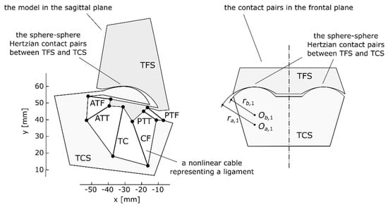
Figure 1.
The assumed symmetrical model of the ankle at rest (at neutral location) in the sagittal plane and a representation of its spherical contact pairs in the frontal plane, reproduced with permission from [10].
- six nonlinear cables substituting the ligaments,
- two Hertzian contact pairs, based on spheres, representing a ball-and-socket joint, which modeled the cartilage,
- two rigid segments representing the tibia/fibula (TFS) and the talus/calcaneus (TCS).
Additionally, the model was assumed to be symmetrical in the sagittal plane. These assumptions reduced a complex three-dimensional structure to a simple two-dimensional counterpart and made it possible to visualize the load state in the joint and analyze the prestrain of the ligaments. In order to ensure that the two-dimensional links joining the bones behaved in a similar fashion to their three-dimensional equivalents, their material parameters were optimized [10].
To specify the relative location of TCS with regard to TFS, three variables were used: two linear coordinates px and py, which formed the translation vector p between the two coordinate frames of the base (TFS) and the moving body (TCS), and the angle θ between the frames used to obtain the rotation matrix R(θ).
The model in Figure 1 corresponded to the ankle at its neutral location (approximately 90 deg between the plane of the foot and the long axis of the tibia). At this location, the model was at rest when no external loads were applied. Furthermore, at this location, the reference frames of TFS and TCS were set to be coincident, which meant that the angle θ was at 0.0 deg, while the linear coordinates px and py were both at 0.0 mm.
2.2. Including Ligament Prestrain in the Model
In the assumed model, a cable i, representing a ligament i, was characterized by five parameters: two position vectors ai, of its attachments to TFS and TCS, two material parameters Ai, Bi and a slack length lslack,i—the length of a retracted ligament after its excision from the joint. Based on these parameters, the value of the force Fi generated by the cable i was obtained using an exponential model [34]:
where li was the current length of the cable, dependent on the location of TCS:
The prestrain was included in the model by shortening the slack lengths of the cables with regards to their lengths when the model was at rest (at the neutral location). In this case, the proportionality ratio between these lengths, corresponded to the prestrain value specified for each ligament:
where: lneutral,i—the length of a ligament j for the model at rest (at the neutral configuration—Figure 1), lslack,i—the slack length of a ligament i, εprestrain,i—the prestrain value for the ligament i (dimensionless).
The length of a ligament lneutral,i could be obtained using (2). Therefore, for a given prestrain value of εprestrain,i, slack length lslack,i was as follows:
Using the equation above it was possible to compute a slack length corresponding to a custom level of prestrain εprestrain,i for each ligament for the model at the neutral location. The computed slack lengths were then used in Equation (1), when computing the forces generated by the ligaments. With this, ligament prestrain was introduced into the model.
The proposed approach was general and could be used for any custom prestrain values. Nevertheless, in this study four approaches were selected—see Table 1. They represented the state-of-the-art in the prestraining methods used in current biomechanical models.

Table 1.
The assumed prestrain values for all the considered prestrain approaches for the ankle at the neutral location.
3. Results
The model was solved under static conditions based on equilibrium equations [10], which were composed from forces/moments generated by the cables and the contact pairs, as well as an external moment acting on TCS.
A detailed summary regarding the computation of the force vectors, their moments and more can be found in [10,12,36,37].
The equilibrium equations were solved numerically with the Levenberg–Marquardt method obtained from SciPy library [38] for the following moment loads:
- Mext = −0.20:0.20 Nm in 51 steps,
- Mext = −5.00:5.00 Nm in 51 steps.
The negative values of the external moment Mext corresponded to dorsiflexion, while the positive moments represented plantarflexion. The obtained solution was considered acceptable, if the sum of the residual loads was less than 1.0 × 10⁻¹⁰.
3.1. The Angular Displacements and the Rest Location
The different variants of prestrain had a significant effect on the angular displacements of the model. In plantarflexion, the relative difference between the considered cases reached up to 10% (see Figure 2a,b).
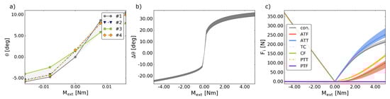
Figure 2.
(a) The angular coordinate θ versus the external moment Mext in the considered prestraining approaches; (b) the angular displacement Δθ versus the external moment Mext in the considered prestraining approaches; (c) the values of the forces Fi generated by the ligaments and the contact pairs versus the external moment Mext in the considered prestraining approaches, where: con. is the magnitude of the contact force generated by the two contact pairs. In all figures: the shaded area corresponds to the minima and the maxima of all the considered prestrain cases.
Interestingly, in cases #2–#4, due to the non-symmetrical distribution, the prestrained ligaments generated an unbalanced net force for the model at the neutral location (see Figure 3). Therefore, in these cases, the model at the neutral location was not at rest, while the “actual” rest location had to be obtained numerically. This affected the reference angle for computing the angular displacement (see Figure 2a) and made the analysis of the results more complex. Furthermore, as seen in Figure 4, to stabilize the model at the “actual” rest location, additional contact forces were necessary.
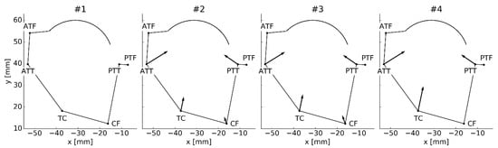
Figure 3.
The ligament forces acting on the TCS at the neutral location of the model. The number above the model corresponds to the prestraining approach. The scale of the vectors was adjusted per drawing for clarity and only relevant parts of the TCS’s contour were drawn.
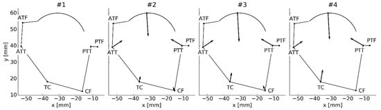
Figure 4.
The ligament forces along with the contact forces stabilizing the TCS at the “actual” computed rest location. The number above the model corresponds to the prestraining approach.
Due to the change in the rest location, the prestrains set at the neutral location and the actual prestrains at the “actual” rest location differed significantly—see Table 2. All of these issues were not a present occurrence in the prestrain-free case #1.
Table 2.
The prestrains assumed for the neutral location and the ones obtained for the “actual” rest location in the prestrain case #3.
3.2. Forces—The Ligaments and the Contact Pairs
The forces generated by most ligaments were largely unaffected by the prestrain as seen in Figure 2c. Nevertheless, significant relative differences of 38% and 19% were recorded for ATT and ATF, respectively. Again, it is worth noting that in the prestrained cases (#2–#4) a contact force was necessary to stabilize the joint (see Figure 4). This force differed in terms of the magnitude between the cases, nevertheless, its direction remained mostly unchanged.
4. Discussion
The presented simulations showcased several interesting behaviors of the ankle joint model under prestrain. The behavior of the prestrained model—cases #2–#4—was difficult to control and analyze.
Firstly, the model experienced a shift in the rest location due to the imbalance of internal loads generated by the prestrained ligaments at the neutral location. This shift in turn affected the reference location for computing the displacement of the model. This presented an extremely serious issue as it rendered the model unpredictable—the rest location under an absence of external loads was dependent on the assumed prestrains.
Secondly, it was impossible to actually enforce the prestrain values on the ligaments. As aforementioned, the prestrains set at the neutral location caused a shift in the rest location. Therefore, the actual prestrains of the ligaments had to be computed at the “actual” rest location and differed from the assumed prestrains at the neutral location. To clarify, the model was prestrained, but the prestrain values were impossible to enforce and were dependent on the “initial” strain values set at the neutral location. It could be concluded that arbitrary prestrain values caused numerical problems with the model and made the analysis of the results much more difficult. These findings suggested that prestrain values were patient specific. It is worth mentioning that these issues were not present for the model with a strain-free configuration—case #1.
The prestrain had a significant effect on the angular displacement, as the maximal relative difference between the angular displacements was 10%, considering all cases. Furthermore, a significant difference was recorded in the behavior of ATT and ATF, as the relative differences between their forces were between 38% and 19%, respectively. This issue should be explored further in future studies.
As mentioned before, in cases #2–#4, the net force generated by the ligaments at the neutral location was unbalanced. In other to balance it, the model had to change its rest location, as shown in Figure 4. Interestingly, the ligaments could not balance themselves. An additional contact force was required. This contact force was generated by the prestrained cartilage in the knee. This further implied that the prestrain was directly connected to the geometry and material parameters of the model. Therefore, arbitrary values of prestrain or even prestrains taken from published experiments could not be valid for most models. The prestrain would require registration along with patient-specific geometry and material parameters of the joint. Nevertheless, this result should be taken with caution, as it could be specific to the model. The assumed model of the cartilage did not account for the friction in the joint. The exact effect of the friction remains, however, difficult to assess, as the friction coefficient can range from 0.002 to 0.500 based on the loads applied on the system [39]. The problem of friction should be considered in future studies.
To summarize, the main novel finding of the study was that the arbitrary prestrain values, commonly employed in biomechanical models of the ankle, cause significant numerical issues with the model, namely:
- a shift in its rest location,
- a difference in its angular displacements and the load state,
- the inability to truly control the assumed prestrain values and, by extension, the model itself.
To the best of my knowledge, an analysis highlighting these problems has never been reported in literature. Furthermore, none of these issues were considered in the papers [2,3,4,5,6,7,8,9] covering biomechanical models. As seen in the results, there was no simple way to introduce ligament prestrain into a model. The actual prestrain values seem to be patient specific, while there remains no viable method to measure them in a noninvasive way. Therefore, based on the performed simulations, a general recommendation is to carefully examine the behavior of the prestrained model near its rest location, as this exemplifies most of the aforementioned issues and could help to estimate their extent. Such an analysis should be taken into account especially, when designing highly-accurate models for surgical planning.
5. Conclusions
The results obtained from the performed prestrain analysis showcased numerical problems when using arbitrary prestrain values for the ligaments in an ankle joint model. The prestrained ligaments, regardless of the prestrain value, caused a shift in the rest location of the model. In this new, shifted location an additional contact force was required to stabilize the joint. Moreover, due to the shift, the prestrains of the ligaments at the rest location differed from the set ones. This proved that the prestrain values were correlated with the geometry and the material parameters of the studied joint. Due to the highly non-symmetrical distribution of ligaments in the joint, setting the prestrains to arbitrary or even experiment-based values rendered the behavior of the model difficult to control, predict and more complex numerically.
The highest difference in the angular displacements was observed at 10% between the considered prestrain cases. Furthermore, the load state in the joint was highly affected by prestrain. For precise models used in presurgical planning this phenomenon should not be omitted. The future work should be focused on further analysis of the prestrain impact on the internal load state of the joint.
To summarize, the problem of prestrain remains difficult to include in biomechanical models. It is advisable to verify the load state in the model at its rest location, which emphasizes the aforementioned problems and can be used to assess their impact on the results.
Funding
This research received no external funding.
Institutional Review Board Statement
Not applicable.
Data Availability Statement
Not applicable.
Acknowledgments
The authors would like to thank the anonymous reviewers for their constructive comments.
Conflicts of Interest
The author declares no conflict of interest.
References
- Maas, S.A.; Erdemir, A.; Halloran, J.P.; Weiss, J.A. A general framework for application of prestrain to computational models of biological materials. J. Mech. Behav. Biomed. Mater. 2016, 61, 499–510. [Google Scholar] [CrossRef] [PubMed]
- Liacouras, P.C.; Wayne, J.S. Computational modeling to predict mechanical function of joints: Application to the lower leg with simulation of two cadaver studies. J. Biomech. Eng. 2007, 129, 811–817. [Google Scholar] [CrossRef]
- Iaquinto, J.M.; Wayne, J.S. Computational model of the lower leg and foot/ankle complex: Application to arch stability. J. Biomech. Eng. 2010, 132, 021009. [Google Scholar] [CrossRef] [PubMed]
- Wei, F.; Hunley, S.C.; Powell, J.W.; Haut, R.C. Development and validation of a computational model to study the effect of foot constraint on ankle injury due to external rotation. Ann. Biomed. Eng. 2011, 39, 756–765. [Google Scholar] [CrossRef] [PubMed]
- Wei, F.; Braman, J.E.; Weaver, B.T.; Haut, R.C. Determination of dynamic ankle ligament strains from a computational model driven by motion analysis based kinematic data. J. Biomech. 2011, 44, 2636–2641. [Google Scholar] [CrossRef]
- Button, K.D.; Wei, F.; Meyer, E.G.; Haut, R.C. Specimen-specific computational models of ankle sprains produced in a laboratory setting. J. Biomech. Eng. 2013, 135, 041001. [Google Scholar] [CrossRef]
- Wei, F.; Fong, D.T.P.; Chan, K.M.; Haut, R.C. Estimation of ligament strains and joint moments in the ankle during a supination sprain injury. Comput. Methods Biomech. Biomed. Eng. 2015, 18, 243–248. [Google Scholar] [CrossRef] [PubMed]
- Purevsuren, T.; Batbaatar, M.; Kim, K.; Park, W.M.; Jang, S.H.; Kim, Y.H. Investigation of ligament strains in lateral ankle sprain using computational simulation of accidental injury cases. J. Mech. Sci. Technol. 2017, 31, 3627–3632. [Google Scholar] [CrossRef]
- Fisk, J.P.; Wayne, J.S. Development and validation of a computational musculoskeletal model of the elbow and forearm. Ann. Biomed. Eng. 2009, 37, 803–812. [Google Scholar] [CrossRef]
- Borucka, A.; Ciszkiewicz, A. A planar model of an ankle joint with optimized material parameters and hertzian contact pairs. Materials 2019, 12, 2621. [Google Scholar] [CrossRef]
- Imhauser, C.W.; Siegler, S.; Udupa, J.K.; Toy, J.R. Subject-specific models of the hindfoot reveal a relationship between morphology and passive mechanical properties. J. Biomech. 2008, 41, 1341–1349. [Google Scholar] [CrossRef] [PubMed]
- Machado, M.; Flores, P.; Claro, J.C.P.; Ambrósio, J.; Silva, M.; Completo, A.; Lankarani, H.M. Development of a planar multibody model of the human knee joint. Nonlinear Dyn. 2009, 60, 459–478. [Google Scholar] [CrossRef]
- Moeinzadeh, M.H.; Engin, A.E.; Akkas, N. Two-dimensional dynamic modelling of human knee joint. J. Biomech. 1983, 16, 253–264. [Google Scholar] [CrossRef]
- Gudavalli, M.R.; Triano, J.J. An analytical model of lumbar motion segment in flexion. J. Manip. Physiol. Ther. 1999, 22, 201–208. [Google Scholar] [CrossRef]
- Forlani, M.; Sancisi, N.; Parenti-Castelli, V. A three-dimensional ankle kinetostatic model to simulate loaded and unloaded joint motion. J. Biomech. Eng. 2015, 137, 061005. [Google Scholar] [CrossRef] [PubMed]
- Beaugonin, M.; Haug, E.; Cesari, D. Improvement of numerical ankle/foot model: Modeling of deformable bone. In Proceedings of the SAE 973331, 41st Stapp Car Crash Conference, Lake Buena Vista, FL, USA, 13–14 November 1997; pp. 225–249. [Google Scholar]
- Klekiel, T.; Będziński, R. Finite element analysis of large deformation of articular cartilage in upper ankle joint of occupant in military vehicles during explosion. Arch. Metall. Mater. 2015, 60, 2115–2121. [Google Scholar] [CrossRef][Green Version]
- Tak-Man Cheung, J.; Zhang, M.; An, K.N. Effects of plantar fascia stiffness on the biomechanical responses of the ankle-foot complex. Clin. Biomech. 2004, 19, 839–846. [Google Scholar] [CrossRef]
- Tannous, R.E.; Bandak, F.A.; Toridis, T.G.; Eppinger, R.H. A three-dimensional finite element model of the human ankle: Development and preliminary application to axial impulsive loading. Proc. Stapp Car Crash Conf. 1996, 40, 219–238. [Google Scholar]
- Delp, S.L.; Anderson, F.C.; Arnold, A.S.; Loan, P.; Habib, A.; John, C.T.; Guendelman, E.; Thelen, D.G. OpenSim: Open-source software to create and analyze dynamic simulations of movement. IEEE Trans. Biomed. Eng. 2007, 54, 1940–1950. [Google Scholar] [CrossRef]
- Dettwyler, M.; Stacoff, A.; Kramers-De Quervain, I.A.; Stüssi, E. Modelling of the ankle joint complex. Reflections with regards to ankle prostheses. Foot Ankle Surg. 2004, 10, 109–119. [Google Scholar] [CrossRef]
- Jamwal, P.K.; Hussain, S.; Tsoi, Y.H.; Ghayesh, M.H.; Xie, S.Q. Musculoskeletal modelling of human ankle complex: Estimation of ankle joint moments. Clin. Biomech. 2017, 44, 75–82. [Google Scholar] [CrossRef] [PubMed]
- Lewis, G.S.; Sommer, H.J.; Piazza, S.J. In vitro assessment of a motion-based optimization method for locating the talocrural and subtalar joint axes. J. Biomech. Eng. 2006, 128, 596. [Google Scholar] [CrossRef] [PubMed]
- Montefiori, E.; Modenese, L.; Di Marco, R.; Magni-Manzoni, S.; Malattia, C.; Petrarca, M.; Ronchetti, A.; de Horatio, L.T.; van Dijkhuizen, P.; Wang, A.; et al. An image-based kinematic model of the tibiotalar and subtalar joints and its application to gait analysis in children with Juvenile Idiopathic Arthritis. J. Biomech. 2019, 85, 27–36. [Google Scholar] [CrossRef] [PubMed]
- van den Bogert, A.J.; Smith, G. In vivo determination of anatomical axes of ankle joint complex. J. Biomech. 1994, 27, 1477–1488. [Google Scholar] [CrossRef]
- Wright, I.C.; Neptune, R.R.; van den Bogert, A.J.; Nigg, B.M. The influence of foot position on ankle sprain. J. Biomech. 2000, 33, 513–519. [Google Scholar] [CrossRef]
- Leardini, A.; O’Connor, J.J.; Catani, F.; Giannini, S. A geometric model of the human ankle joint. J. Biomech. 1999, 32, 585–591. [Google Scholar] [CrossRef]
- Ratajczak, M.; Ptak, M.; Kwiatkowski, A.; Kubicki, K.; Fernandes, F.A.O.; Wilhelm, J.; Dymek, M.; Sawicki, M.; Żółkiewski, S. Symmetry of the human head—Are symmetrical models more applicable in numerical analysis? Symmetry 2021, 13, 1252. [Google Scholar] [CrossRef]
- Gregorio, R.; Parenti-Castelli, V.; O’Connor, J.J.; Leardini, A. Mathematical models of passive motion at the human ankle joint by equivalent spatial parallel mechanisms. Med. Biol. Eng. Comput. 2007, 45, 305–313. [Google Scholar] [CrossRef]
- Franci, R.; Parenti-Castelli, V. A 5-5 One-degree-of-freedom fully parallel mechanism for the modeling of passive motion at the human ankle joint. In Proceedings of the ASME 2007 International Design Engineering Technical Conferences & Computers and Information in Engineering Conference IDETC/CIE 2007, Las Vegas, NV, USA, 4–7 September 2007; pp. 637–644. [Google Scholar]
- Sancisi, N.; Parenti-Castelli, V. A 1-dof parallel spherical wrist for the modelling of the knee passive motion. Mech. Mach. Theory 2010, 45, 658–665. [Google Scholar] [CrossRef]
- Ciszkiewicz, A.; Knapczyk, J. Load analysis of a patellofemoral joint by a quadriceps muscle. Acta Bioeng. Biomech. 2016, 18, 111–119. [Google Scholar]
- Ciszkiewicz, A. Analyzing uncertainty of an ankle joint model with genetic algorithm. Materials 2020, 13, 1175. [Google Scholar] [CrossRef] [PubMed]
- Funk, J.R.; Hall, G.W.; Crandall, J.R.; Pilkey, W.D. Linear and quasi-linear viscoelastic characterization of ankle ligaments. J. Biomech. Eng. 2002, 122, 15. [Google Scholar] [CrossRef] [PubMed]
- Ozeki, S.; Yasuda, K.; Yamakoshi, K.; Yamanoi, T. Simultaneous strain measurement with determination of a zero strain reference for the medial and lateral ligaments of the ankle. Foot Ankle Int. 2002, 825–832. [Google Scholar] [CrossRef] [PubMed]
- Ciszkiewicz, A.; Milewski, G. Structural and material optimization for automatic synthesis of spine-segment mechanisms for humanoid robots with custom stiffness profiles. Materials 2019, 12, 1982. [Google Scholar] [CrossRef] [PubMed]
- Hertz, H. On the contact of solids—on the contact of rigid elastic solids and on hardness. In Miscellaneous Papers; Macmillan: London, UK, 1896; pp. 146–183. [Google Scholar]
- van der Walt, S.; Colbert, S.C.; Varoquaux, G. The NumPy array: A structure for efficient numerical computation. Comput. Sci. Eng. 2011, 13, 22–30. [Google Scholar] [CrossRef]
- Oungoulian, S.R.; Durney, K.M.; Jones, B.K.; Ahmad, C.S.; Hung, C.T.; Ateshian, G.A. Wear and damage of articular cartilage with friction against orthopaedic implant materials. J. Biomech. 2015, 48, 1957–1964. [Google Scholar] [CrossRef]
Publisher’s Note: MDPI stays neutral with regard to jurisdictional claims in published maps and institutional affiliations. |
© 2022 by the author. Licensee MDPI, Basel, Switzerland. This article is an open access article distributed under the terms and conditions of the Creative Commons Attribution (CC BY) license (https://creativecommons.org/licenses/by/4.0/).