A Constrained Shepard Type Operator for Modeling and Visualization of Scattered Data ^†

Abstract

For solving the problem of modeling and visualization of scattered data that should preserve some constraints, we use a modified Shepard type operator that is required to fulfill some special conditions, highlighting the symmetry with other methods. We illustrate the properties of the obtained operators by some numerical examples.

1. Introduction

Some of the most important interpolation methods for large scattered data sets are the Shepard type methods. The problem of modeling and visualization of scattered data that should preserve some constraints appears in many scientific areas, e.g., when the data should satisfy lower and upper bounds, due to various constraints (economical, physical, socio-political, chemical, etc. [1]). For example, there are cases when the data have to preserve some constraints, subject to certain physical laws (e.g., the densities, percentage mass concentrations in a chemical reaction, volume and mass, see [2,3]). Such problems require to impose some special conditions to the interpolants (see, e.g., [1,2,3,4]).

The purpose of the paper is to impose some constraints to Shepard-Bernoulli operator, introduced in [5], and to enforce it to satisfy them using a symmetrical way with the method described in [1]. First, we recall some results regarding Shepard-Bernoulli interpolation, studied in [5,6,7].

Consider the function $f\in C^{(m,n)}\left(X\right),$$X=[a,b]\times [c,d]$ and a set of N distinct points $(x_i,y_i)\in X,i=1,...,N.$ The bivariate Shepard operator (introduced in [8]) is given by

$$Sf\left(x,y\right)=\sum _{i=1}^N{A}_i\left(x,y\right)f\left(x_i,y_i\right),$$

(1)

where

$$A_i\left(x,y\right)=\frac{{\displaystyle \prod _{\begin{array}{c}j=1\\ j\ne i\end{array}}^N}{r}_j^{\mu }\left(x,y\right)}{{\displaystyle \sum _{k=1}^N}{\displaystyle \prod _{\begin{array}{c}j=1\\ j\ne k\end{array}}^N}{r}_j^{\mu }\left(x,y\right)},$$

(2)

with $\mu >0$ and $r_i\left(x,y\right)$ are the distances between $\left(x,y\right)$ and the given points $\left(x_i,y_i\right),i=1,...,N$. The parameter $\mu$ influences the behavior of $Sf$ in the neighborhood of the nodes. If $0<\mu \le 1$ then $Sf$ has peaks at the nodes. For $\mu >1$ then $Sf$ has flat spots and if $\mu$ is large enough $Sf$ becomes a step function.

Proposition 1.

The following properties hold:

• $A_i\left(x_k,y_k\right)={\delta }_{ik},$$i,k=1,...,N.$
• degree of exactness of S is 0 ($dex\left(S\right)=0).$

Shepard interpolation leads to flat spots at each data point and the accuracy tends to decrease in the areas where the interpolation nodes are sparse. This can be improved using the local version of Shepard interpolation, introduced by Franke and Nielson in [9] and improved in [10,11,12]:

$$Sf\left(x,y\right)=\frac{{\displaystyle \sum _{i=1}^N}{W}_i\left(x,y\right)f\left(x_i,y_i\right)}{{\displaystyle \sum _{i=1}^N}{W}_i\left(x,y\right)},$$

(3)

with

$$W_i\left(x,y\right)={\left[{\displaystyle \frac{{(R_w-r_i(x,y))}_{+}}{R_w{r}_i(x,y)}}\right]}^2,$$

(4)

where $R_w$ is a radius of influence about the node $(x_i,y_i)$ and it is varying with $i.$ This is taken as the distance from node i to the jth closest node to $(x_i,y_i)$ for $j>N_w$ ($N_w$ is a fixed value) and j as small as possible within the constraint that the jth closest node is significantly more distant than the $(j-1)$st closest node (see, e.g., [11]).

The Bernoulli polynomials are defined by (see, e.g., [13]):

$$\left\{\begin{array}{cc}{B}_0\left(x\right)=1,\hfill & \\ B_n^{\prime }\left(x\right)=n{B}_{n-1}\left(x\right),\hfill & n\ge 1,\\ {\displaystyle {\int }_0^1}{B}_n\left(x\right)dx=0,\hfill & n\ge 1.\end{array}\right.$$

(5)

The values of $B_n\left(x\right)$ at $x=0$ are the Bernoulli numbers and they are denoted by $B_n.$ For $f\in C^m[a,b],$ the univariate Bernoulli interpolant is given by

$$B_{m}f\left(x\right):=B_m[f;a,b]=f\left(a\right)+\sum _{i=1}^m{S}_i\left({\displaystyle \frac{x-a}{h}}\right){\displaystyle \frac{h^{i-1}}{i!}}{\Delta }_h{f}^{(i-1)}\left(a\right),$$

(6)

where $h=b-a$ and

$$\begin{array}{cc}\hfill & S_i\left({\displaystyle \frac{x-a}{h}}\right)=B_i\left({\displaystyle \frac{x-a}{h}}\right)-B_i,i\ge 1,\hfill \\ \hfill & {\Delta }_h{f}^{(i-1)}\left(a\right)=f^{(i-1)}\left(b\right)-f^{(i-1)}\left(a\right),1\le i\le m.\hfill \end{array}$$

(7)

Denote $h:=b-a,$$k:=d-c$ and consider the operators:

$$\begin{array}{cc}\hfill {\Delta }_{(h,0)}f(x,y)& :=f(x+h,y)-f(x,y),\hfill \\ \hfill {\Delta }_{(0,k)}f(x,y)& :=f(x,y+k)-f(x,y),\hfill \\ \hfill {\Delta }_{(h,k)}f(x,y)& :={\Delta }_{(h,0)}{\Delta }_{(0,k)}f(x,y)={\Delta }_{(0,k)}{\Delta }_{(h,0)}f(x,y).\hfill \end{array}$$

(8)

For $f\in C^{m,n}\left(X\right),$ the Bernoulli interpolant on the rectangle is [13]:

$$\begin{array}{cc}\hfill B_{m,n}f(x,y):=& f(a,c)+\sum _{i=1}^m{\Delta }_{(h,0)}{f}^{(i-1,0)}(a,c){\displaystyle \frac{h^{i-1}}{i!}}{S}_i\left({\displaystyle \frac{x-a}{h}}\right)\hfill \\ \hfill & +\sum _{j=1}^n{\Delta }_{(0,k)}{f}^{(0,j-1)}(a,c){\displaystyle \frac{k^{j-1}}{j!}}{S}_j\left({\displaystyle \frac{y-c}{k}}\right)\hfill \\ \hfill & +\sum _{i=1}^m\sum _{j=1}^n{\Delta }_{(h,k)}{f}^{(i-1,j-1)}(a,c){\displaystyle \frac{h^{i-1}{k}^{j-1}}{i!j!}}{S}_i\left({\displaystyle \frac{x-a}{h}}\right)S_j\left({\displaystyle \frac{y-c}{k}}\right),\hfill \end{array}$$

(9)

where $S_k,$$k>1$ are given in (7). The polynomial from (9) satisfies the following interpolation conditions:

$$\begin{array}{cc}\hfill B_{m,n}f(a,c)& =f(a,c),\hfill \\ \hfill {\left({\Delta }_{(h,0)}{B}_{m,n}f\right)}^{(i,0)}(a,c)& ={\Delta }_{(h,0)}{f}^{(i,0)}(a,c),0\le i\le m-1,\hfill \\ \hfill {\left({\Delta }_{(0,k)}{B}_{m,n}f\right)}^{(0,j)}(a,c)& ={\Delta }_{(0,k)}{f}^{(0,j)}(a,c),0\le j\le n-1,\hfill \\ \hfill {\left({\Delta }_{(h,k)}{B}_{m,n}f\right)}^{(i,j)}(a,c)& ={\Delta }_{(h,k)}{f}^{(i,j)}(a,c),0\le i\le m-1,0\le j\le n-1.\hfill \end{array}$$

(10)

The bivariate Shepard-Bernoulli operator (introduced in [5]) preserves the advantages and improve the reproduction qualities, have better accuracy and computational efficiency:

$$S_{B}f(x,y)=\sum _{i=1}^N{A}_i(x,y)B_{m,n}^{i}f(x,y),\mu >0,$$

(11)

where $B_{m,n}^{i}f$ denotes the Bernoulli interpolant $B_{m,n}[f;(x_i,y_i),(h_i,k_i)]$ in the rectangle with opposite vertices $(x_i,y_i),$$(x_{i+1},y_{i+1})$, given by (9), having $h_i=x_{i+1}-x_i$, $k_i=y_{i+1}-y_i,$$i=1,...,N$.

The improved form of the Shepard-Bernoulli operator, based on (3), is (see [5]):

$$S_B^{w}f\left(x,y\right):=\frac{{\displaystyle \sum _{i=1}^N}{W}_i\left(x,y\right)B_{m,n}^{i}f(x,y)}{{\displaystyle \sum _{i=1}^N}{W}_i\left(x,y\right)}.$$

(12)

2. Constraints of the Shepard-Bernoulli Operator

Consider the function $f\in C^{(m,n)}\left(X\right),$$X=[a,b]\times [c,d]$ and a set of N distinct points $(x_i,y_i)\in X,i=1,...,N.$ The classical Shepard operator $S,$ given in (1) satisfies the following property:

$$\underset{i=1,...,N}{min}\left\{f\left(x_i,y_i\right)\right\}\le Sf(x,y)\le \underset{i=1,...,N}{max}\left\{f\left(x_i,y_i\right)\right\}.$$

(13)

A consequence of this property is that a positive interpolant is guaranteed if the data values are positive.

The modified Shepard operator, given in (3), has superior qualities but it does not satisfy the property (13).

We will impose constraints to the operators given in (11) and (12) using the steps of the method described in [1], whose notations will be used.

Let $C_U$ and $C_L$ be the upper and lower bounds in $\mathbb{R}$, a constant K in $(0,1)$ and $p=\frac{1}{K}-1.$ We mention that K is an input parameter which gives us flexibility to use a value suitable for the application. We consider

$$\begin{array}{cc}\hfill d_U(x_i,y_i)& :=f(x_i,y_i)-C_U,\hfill \\ \hfill d_L(x_i,y_i)& :=f(x_i,y_i)-C_L,\hfill \\ \hfill D_U(x_i,y_i)& :=d_U(x_i,y_i)+K[B_{m,n}^{i}f(x,y)-f(x_i,y_i)],\hfill \\ \hfill D_L(x_i,y_i)& :=d_L(x_i,y_i)+K[B_{m,n}^{i}f(x,y)-f(x_i,y_i)],\hfill \\ \hfill Q(x_i,y_i)& :=f(x_i,y_i)+K[B_{m,n}^{i}f(x,y)-f(x_i,y_i)],\hfill \end{array}$$

and

$${\mu }_U(x_i,y_i):=\left\{\begin{array}{cc}{\left(\frac{D_U(x_i,y_i)}{d_U(x_i,y_i)}\right)}^p,\hfill & \mathrm{if}f(x_i,y_i)\le B_{m,n}^{i}f(x_i,y_i)\le C_U,\hfill \\ 0,\hfill & \mathrm{otherwise}.\hfill \end{array}\right.$$

(14)

$${\mu }_L(x_i,y_i):=\left\{\begin{array}{cc}{\left(\frac{D_L(x_i,y_i)}{d_L(x_i,y_i)}\right)}^p,\hfill & \mathrm{if}{C}_L\le B_{m,n}^{i}f(x_i,y_i)\le f(x_i,y_i)\hfill \\ 0,\hfill & \mathrm{otherwise}.\hfill \end{array}\right.$$

(15)

Let

$$R(x_i,y_i)=\left\{\begin{array}{cc}{C}_U+{\mu }_U(x_i,y_i)D_U(x_i,y_i),\hfill & \mathrm{if}f(x_i,y_i)\le B_{m,n}^{i}f(x_i,y_i),\hfill \\ C_L+{\mu }_L(x_i,y_i)D_L(x_i,y_i),\hfill & \mathrm{otherwise}.\hfill \end{array}\right.$$

(16)

The constrained Shepard-Bernoulli operators are given by

$$S_{c_1}f\left(x,y\right)=\sum _{i=1}^N{A}_i\left(x,y\right)R\left(x_i,y_i\right),$$

(17)

$$S_{c_2}f\left(x,y\right)={\displaystyle \frac{{\displaystyle \sum _{i=1}^N}{W}_i\left(x,y\right)R\left(x_i,y_i\right)}{{\displaystyle \sum _{i=1}^N}{W}_i\left(x,y\right)}},$$

(18)

with $A_i\left(x,y\right)$ and $W_i\left(x,y\right)$ given by (2) and (4), respectively.

Theorem 1.

For $(x,y)\in X,$ it holds

$$C_L\le S_{c1}f\left(x,y\right)\le C_U,$$

(19)

and

$$C_L\le S_{c2}f\left(x,y\right)\le C_U.$$

(20)

Proof. 

Replacing (14) and (15) in (16), we get

$$\begin{array}{cc}\hfill & R(x_i,y_i)=\hfill \\ \hfill & =\left\{\begin{array}{cc}{C}_U+{\displaystyle \frac{{(f(x_i,y_i)-C_U+K(B_{m,n}^{i}f(x,y)-f(x_i,y_i)))}^{p+1}}{{(f(x_i,y_i)-C_U)}^p}},\hfill & \mathrm{if}f(x_i,y_i)\le B_{m,n}^{i}f(x_i,y_i)\le C_U\hfill \\ C_L+{{\displaystyle \frac{(f(x_i,y_i)-C_L+K(B_{m,n}^{i}f(x,y)-f(x_i,y_i)))}{{(f(x_i,y_i)-C_L)}^p}}}^{p+1},\hfill & \mathrm{if}{C}_L\le B_{m,n}^{i}f(x_i,y_i)\le f(x_i,y_i).\hfill \end{array}\right.\hfill \end{array}$$

If $f(x_i,y_i)\le B_{m,n}^{i}f(x_i,y_i)\le C_U,$ it holds

$$\begin{array}{cc}\hfill R(x_i,y_i)& \le C_U+{\displaystyle \frac{{(f(x_i,y_i)-C_U+B_{m,n}^{i}f(x,y)-f(x_i,y_i))}^{p+1}}{{(f(x_i,y_i)-C_U)}^p}}\hfill \\ \hfill & \le C_U+{\left({\displaystyle \frac{B_{m,n}^{i}f(x,y)-C_U}{f(x_i,y_i)-C_U}}\right)}^p(B_{m,n}^{i}f(x,y)-C_U)\le C_U.\hfill \end{array}$$

If $C_L\le B_{m,n}^{i}f(x_i,y_i)\le f(x_i,y_i),$ it holds

$$R(x_i,y_i)\ge C_L+f(x_i,y_i)-C_L\ge f(x_i,y_i)\ge C_L.$$

Therefore, by (17) and (2), the inequality (19) is proved.

Similarly, taking into account (18) and (4), (20) follows. □

Theorem 2.

For $f\in C^{(m,n)}\left(X\right),$ the following interpolation properties hold:

$$S_{c1}^{}f(x_k,y_k)=f(x_k,y_k),$$

for $1\le k\le N$ and $\mu >m+n-2.$

Proof. 

We have

$$S_{c_1}^{}f(x_k,y_k)=\sum _{i=1}^N{A}_i\left(x_k,y_k\right)R\left(x_i,y_i\right)$$

and by the property $A_i\left(x_k,y_k\right)={\delta }_{ik},$ see Proposition 1, we get

$$\begin{array}{cc}\hfill S_{c_1}^{}f& (x_k,y_k)=R\left(x_k,y_k\right)\hfill \\ \hfill & =\left\{\begin{array}{cc}{C}_U+{\left({\displaystyle \frac{D_U(x_k,y_k)}{d_U(x_k,y_k)}}\right)}^p{D}_U(x_k,y_k),\hfill & \mathrm{if}f(x_k,y_k)\le Q(x_k,y_k),\hfill \\ C_L+{\left({\displaystyle \frac{D_L(x_k,y_k)}{d_L(x_k,y_k)}}\right)}^p{D}_L(x_k,y_k),\hfill & \mathrm{otherwise}.\hfill \end{array}\right.\hfill \\ \hfill & =\left\{\begin{array}{cc}{C}_U+{\displaystyle \frac{{(d_U(x_k,y_k)+K(B_{m,n}^{k}f(x,y)-f(x_k,y_k)))}^{p+1}}{{\left[d_U(x_k,y_k)\right]}^p}},\hfill & \mathrm{if}f(x_k,y_k)\le Q(x_k,y_k),\hfill \\ C_L+{\displaystyle \frac{{(d_L(x_k,y_k)+K(B_{m,n}^{k}f(x,y)-f(x_k,y_k)))}^{p+1}}{{\left[d_L(x_k,y_k)\right]}^p}},\hfill & \mathrm{otherwise}.\hfill \end{array}\right.\hfill \end{array}$$

By the interpolation properties of the Bernoulli operator, we have $B_{m,n}^{k}f(x_k,y_k)=f(x_k,y_k),$ for $k=1,...,N,$ whence it follows

$$\begin{array}{cc}\hfill \left(S_{c_1}^{}f\right)(x_k,y_k)& =\left\{\begin{array}{cc}{C}_U+d_U(x_k,y_k),\hfill & \mathrm{if}f(x_k,y_k)\le Q(x_k,y_k)\hfill \\ C_L+d_L(x_k,y_k),\hfill & \mathrm{otherwise}.\hfill \end{array}\right.\hfill \\ \hfill & =f(x_k,y_k),\mathrm{for}k=1,...,N.\hfill \end{array}$$

□

Theorem 3.

The degree of exactness of the operator $S_{c_1}^{}$ is $0.$

Proof. 

Considering $e_{k,j}(x,y)=x^k{y}^j,$ with $k\le m$ and $j\le n,$ we have

$$\begin{array}{cc}\hfill & S_{c_1}{e}_{k,j}\left(x,y\right)=\sum _{i=1}^N{A}_i\left(x,y\right)R\left(x_i,y_i\right)\hfill \\ \hfill & =\left\{\begin{array}{cc}{C}_U+{\displaystyle \sum _{i=1}^N}{A}_i\left(x,y\right){\left({\displaystyle \frac{D_U(x_i,y_i)}{d_U(x_i,y_i)}}\right)}^p{D}_U(x_i,y_i),\hfill & \mathrm{if}f(x_i,y_i)\le Q(x_i,y_i),\hfill \\ C_L+{\displaystyle \sum _{i=1}^N}{A}_i\left(x,y\right){\left({\displaystyle \frac{D_L(x_i,y_i)}{d_L(x_i,y_i)}}\right)}^p{D}_L(x_i,y_i),\hfill & \mathrm{otherwise}.\hfill \end{array}\right.\hfill \\ \hfill & =\left\{\begin{array}{cc}{C}_U+{\displaystyle \sum _{i=1}^N}{\displaystyle \frac{A_i\left(x,y\right){(d_U(x_i,y_i)+K(B_{m,n}^i{e}_{k,j}(x,y)-e_{k,j}(x_i,y_i)))}^{p+1}}{{\left(d_U(x_i,y_i)\right)}^p}},\hfill & \mathrm{if}f(x_i,y_i)\le Q(x_i,y_i),\hfill \\ C_L+{\displaystyle \sum _{i=1}^N}{\displaystyle \frac{A_i\left(x,y\right){(d_L(x_i,y_i)+K(B_{m,n}^i{e}_{k,j}(x,y)-e_{k,j}(x_i,y_i)))}^{p+1}}{{\left(d_L(x_i,y_i)\right)}^p}},\hfill & \mathrm{otherwise}.\hfill \end{array}\right.\hfill \end{array}$$

Having degree of exactness of $B_{m,n}^i$ equal to $(m,n)$ (see, e.g., [5,13]), for $k\le m$ and $j\le n,$ we get

$$\begin{array}{cc}\hfill S_{c_1}{e}_{k,j}& \left(x,y\right)=\left\{\begin{array}{cc}{C}_U+{\displaystyle \sum _{i=1}^N}{A}_i\left(x,y\right)d_U(x_i,y_i),\hfill & \mathrm{if}f(x_i,y_i)\le Q(x_i,y_i)\hfill \\ C_L+{\displaystyle \sum _{i=1}^N}{A}_i\left(x,y\right)d_L(x_i,y_i),\hfill & \mathrm{otherwise}.\hfill \end{array}\right.\hfill \\ \hfill & =\left\{\begin{array}{cc}{C}_U+{\displaystyle \sum _{i=1}^N}{A}_i\left(x,y\right)(e_{k,j}(x_i,y_i)-C_U),\hfill & \mathrm{if}f(x_i,y_i)\le Q(x_i,y_i)\hfill \\ C_L+{\displaystyle \sum _{i=1}^N}{A}_i\left(x,y\right)(e_{k,j}(x_i,y_i)-C_L),\hfill & \mathrm{otherwise}.\hfill \end{array}\right.\hfill \end{array}$$

Applying the property that $dex\left(S\right)=0$ (see Proposition 1), we get $S_{c_1}{e}_{k,j}\left(x,y\right)=e_{k,j}(x,y)$ for $k=j=0.$ □

3. Numerical Examples

To illustrate the performance of the proposed constructions, we consider the following test functions ([10,11,12]):

$$\begin{array}{cc}\hfill \mathrm{Gentle}:f_1(x,y)=& exp[-{\displaystyle \frac{81}{16}}({(x-0.5)}^2+{(y-0.5)}^2)]/3,\hfill \\ \hfill \mathrm{Saddle}:f_2(x,y)=& {\displaystyle \frac{(1.25+cos5.4y)}{6+6{(3x-1)}^2}},\hfill \\ \hfill \mathrm{Franke}:f_3(x,y)=& 0.75e^{-\frac{1}{4}[{(9x-2)}^2+{(9y-2)}^2]}+0.75e^{[-\frac{1}{49}{(9x+1)}^2-\frac{1}{10}(9y+1)]}\hfill \\ \hfill & +0.5e^{-\frac{1}{4}[{(9x-7)}^2+{(9y-3)}^2]}-0.2e^{[-{(9x-4)}^2-{(9y-7)}^2]}.\hfill \end{array}$$

Table 1 shows the minimum and the maximum values of $S_{c_{{}_2}}{f}_i,$ $i=1,2,3,$ for cases $C_L=0;$ $C_U=1$ and $C_L=0;$ $C_U=2$, considering 20 random generated nodes, $K=0.5$ and $N_w=8.$

Table 1. Minimum and maximum of $S_{c_2^{}}{f}_i,$$i=1,2,3$.

	${\mathit{C}}_{\mathit{L}}=0;$  ${\mathit{C}}_{\mathit{U}}=1$		${\mathit{C}}_{\mathit{L}}=0;$  ${\mathit{C}}_{\mathit{U}}=2$
	min	max	min	max
$S_{c_2}{f}_1$	$0.0274$	$0.3479$	0	$0.5167$
$S_{c_2}{f}_2$	$0.0103$	$0.6163$	$6.7525\times {10}^4$	$0.3590$
$S_{c_2}{f}_3$	$0.0346$	$0.9959$	$1.0621\times {10}^4$	$1.7136$

In Figure 1, Figure 2 and Figure 3 we plot the graphs of $f_i,$$S_B^w{f}_i,$ $S_{c_{{}_2}}{f}_i,$ for $i=1,2,3$ (that have better approximation properties than $S_{c_{{}_1}}{f}_i$).

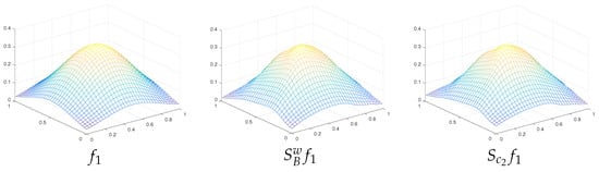
Figure 1. Graphs for $f_1$.

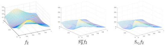
Figure 2. Graphs for $f_2$.

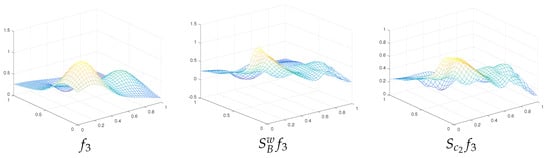
Figure 3. Graphs for $f_3$.

4. Conclusions

By Table 1, we remark that the values of $S_{c_2}{f}_i,$$i=1,2,3$ preserve the lower bound of $C_L$ and the upper bound of $C_U,$ as it is theoretically proved in the previous section. Further, by the same table and the figures, we note the good approximation properties of the constructed operators.

By Figure 1, Figure 2 and Figure 3, it is seen that the behaviour of the operators $S_{c_2}{f}_i,$$i=1,2,3$, is better than the behaviour of the improved form of the Shepard-Bernoulli operators, $S_B^w{f}_i,$$i=1,2,3$.

References

- Mustafa, G.; Shah, A.A.; Asim, M.R. Constrained Shepard method for modeling and visualization of scattered data. In Proceedings of the WSCG 2008, Plzen, Czech Republic, 4–7 February 2008; Science Press: Plzen, Csech Republic, 2008; Volume 16, pp. 49–56. [Google Scholar]
- Asim, M.R.; Mustafa, G.; Brodlie, K.W. Constrained Visualization of 2D Positive Data using Modified Quadratic Shepard Method. In Proceedings of the WSCG 2004, Plzen-Bory, Czech Republic, 2–6 February 2004; Science Press: Plzen, Czech Republic, 2004; pp. 9–13. [Google Scholar]
- Brodlie, K.W.; Asim, M.R.; Unsworth, K. Constrained Visualization Using the Shepard Interpolation Family. Comput. Graph. Forum 2005, 24, 809–820. [Google Scholar] [CrossRef]
- Cătinaş, T. Constrained visualisation using Shepard-Bernoulli interpolation operator. Stud. Univ. Babes-Bolyai Math. 2020, 65, 269–277. [Google Scholar] [CrossRef]
- Cătinaş, T. The bivariate Shepard operator of Bernoulli type. Calcolo 2007, 44, 189–202. [Google Scholar] [CrossRef]
- Caira, R.; Dell’Accio, F. Shepard–Bernoulli operators. Math. Comp. 2007, 76, 299–321. [Google Scholar] [CrossRef]
- Dell’Accio, F.; Tommaso, F.D. Bivariate Shepard–Bernoulli operators. Math. Comput. Simul. 2017, 141, 65–82. [Google Scholar] [CrossRef] [Green Version]
- Shepard, D. A two dimensional interpolation function for irregularly spaced data. In Proceedings of the 23rd ACM National Conference, New York, NY, USA, 27–29 August 1968; pp. 517–523. [Google Scholar]
- Franke, R.; Nielson, G. Smooth interpolation of large sets of scattered data. Int. J. Numer. Meths. Engrg. 1980, 15, 1691–1704. [Google Scholar] [CrossRef]
- Franke, R. Scattered data interpolation: Tests of some methods. Math. Comp. 1982, 38, 181–200. [Google Scholar]
- Renka, R.J. Multivariate interpolation of large sets of scattered data. ACM Trans. Math. Softw. 1988, 14, 139–148. [Google Scholar] [CrossRef]
- Renka, R.J.; Cline, A.K. A triangle-based C1 interpolation method. Rocky Mt. J. Math. 1984, 14, 223–237. [Google Scholar] [CrossRef]
- Costabile, F.A.; Dell’Accio, F. Expansion Over a Rectangle of Real Functions in Bernoulli Polynomials and Applications. BIT 2001, 41, 451–464. [Google Scholar] [CrossRef]
Publisher’s Note: MDPI stays neutral with regard to jurisdictional claims in published maps and institutional affiliations. |
© 2022 by the author. Licensee MDPI, Basel, Switzerland. This article is an open access article distributed under the terms and conditions of the Creative Commons Attribution (CC BY) license (https://creativecommons.org/licenses/by/4.0/).