A Motion Planning Method for Automated Vehicles in Dynamic Traffic Scenarios

Abstract

We propose a motion planning method for automated vehicles (AVs) to complete driving tasks in dynamic traffic scenes. The proposed method aims to generate motion trajectories for an AV after obtaining the surrounding dynamic information and making a preliminary driving decision. The method generates a reference line by interpolating the original waypoints and generates optional trajectories with costs in a prediction interval containing three dimensions (lateral distance, time, and velocity) in the Frenet frame, and filters the optimal trajectory by a series of threshold checks. When calculating the feasibility of optional trajectories, the cost of all optional trajectories after removing obstacle interference shows obvious axisymmetric regularity concerning the reference line. Based on this regularity, we apply the constrained Simulated Annealing Algorithm (SAA) to improve the process of searching for the optimal trajectories. Experiments in three different simulated driving scenarios (speed maintaining, lane changing, and car following) show that the proposed method can efficiently generate safe and comfortable motion trajectories for AVs in dynamic environments. Compared with the method of traversing sampling points in discrete space, the improved motion planning method saves 70.23% of the computation time, and overcomes the limitation of the spatial sampling interval.

1. Introduction

As an important aspect of profiling the evolution of human civilization, transportation modalities are rapidly moving towards automation and interconnection. It is widely accepted that transportation systems will become much more efficient and safer when the task of vehicle driving shifts from a manual process to an automatic process. Over the past few decades, researchers have devoted a great deal of effort to realize the goal of autopiloting. The current process of achieving autonomous driving consists of environment perception and localization, behavior decisions, motion planning, and trajectory tracking. The purpose of motion planning is to generate a trajectory that satisfies the constraints of vehicle dynamics, driving safety, comfort, and efficiency, after the AV makes the next initial driving decision based on dynamic environment information and its state. Motion planning is a key part of the autonomous driving technology process and a critical factor in drivers’ experience and safety.

1.1. Related Work

The methods of motion planning for AVs originally evolved from mobile robot technology [1,2,3,4]. As autopilot technology has gradually developed, numerous motion planning methods have become available for AVs [5]. Originally applied from the field of mobile robotics to the field of automated vehicles, the Graph Searching-based method has a strong path searching capability in complex spaces [6,7,8]. However, it is often difficult for this method to satisfy the dynamics constraints of AVs because the movable degrees of freedom of AVs are much less than those of robots, and the speed of AVs far exceeds that of robots. The State Lattice method is a path planning method based on graph searching and sampling [9,10], and has been widely used in the obstacle avoidance planning of AVs and shown good results in the DARPA urban challenge [11]. However, the path selection of the State Lattice method is relatively simple in the complex road environment. As a result, it has difficulty in approaching the optimal solution in some cases. The artificial potential field method was first proposed by Khatib [12]. This method uses the attraction of the target point and the repulsion of the obstacle to guide the vehicle safely to the target point [13,14,15,16]. Because of the local minimum problem, vehicles are easily trapped in the local minimum of the potential field. The Interpolating Curve-based method describes the path under the constraints of vehicle dynamics [17,18,19], but tends to ignore the problem of traffic environment changes in the process of trajectory planning, and has poor ability to deal with dynamic obstacle interference. Therefore, the Interpolating Curve-based method is often used in the process of trajectory smoothing and optimization. The sampling-based method uses a large number of samples in the complex search space and can quickly find the passable path in the workspace [20,21]. However, because the sampling points cannot cover the whole planning space, it is difficult for this method to find the optimal or suboptimal path.

The method of sampling-based motion planning in the Frenet frame was first proposed by Werling [22,23], and has been widely adopted due to its simplicity and effectiveness. In this method, the Frenet frame based on the road center line was used to describe the lateral and longitudinal motions of the AV, and the time-varying polynomial was used to generate trajectories to ensure comfort. The optimal trajectory was then found by an exhaustive method. However, due to this method’s complexity, caused by traversing each trajectory, its performance depends on the number of sampling points in the sampling space. The key problem is to balance the calculation of the algorithm and the precision of the sampling space [24,25]. In [26], the sampling space of the motion planning method was discretized and dimensionally reduced, and the path and speed of the synthetic trajectory were iteratively optimized, and the complexity of the algorithm was reduced. The cost function and polygon constraints of the motion planning method were optimized in [27], and the numerical optimization algorithm was adopted to improve the comfort degree of the trajectory. Numerical optimization methods are often combined with other methods to optimize trajectories. A path/speed decoupled trajectory optimization was proposed in [28], and a path planning method through an optimal controller integrating obstacle-dependent Gaussian and model prediction control was proposed in [16]. The performance of the sampling-based motion planning method in the Frenet frame under static and dynamic obstacle scenarios was discussed in detail in [29]. Sampling and Graph Searching-based methods in the Frenet frame were combined in [30], and part of the trajectory searching space was simplified to improve efficiency. Lazy collision-checking was applied to reduce the time required for trajectory checking in [31]. The motion planning problem was divided into two steps of lateral motion sampling and longitudinal numerical optimization in [32], and the generation of longitudinal trajectories was accelerated by the Model Predictive Control method. Short-term motion planning based on the Frenet frame and long-term decision making was combined in [33]. The results showed that the Frenet frame performs well in the simulated traffic flow. The continuous spatiotemporal trajectories were generated on the Frenet frame based on deep learning in [34], and the validity of the framework was tested in a large number of randomly generated valid scenarios.

All of these studies were aimed at improving the efficiency of motion planning methods for the AVs. The most important factor affecting the complexity of the sampling-based motion planning method in the Frenet frame is the number of optional trajectories during the execution process; that is, the key to improving the efficiency is to quickly find the optimal trajectory from the sampling space. In addition, increasing the speed by decreasing the density of sampling points may lead to a decrease in the accuracy of the motion planning method, due to the fact that reducing the sampling points may cause the optimal trajectory to be missed. Achieving a balance between the number of optional trajectories in the sampling space and the efficiency of the method has rarely been mentioned in previous studies.

1.2. Contribution

To overcome these limitations, this paper proposes a safe and efficient motion planning method for dynamic traffic scenes by combining the sampling-based method in the Frenet frame and the optimal trajectory searching method improved by SAA. The motion planning is divided into two parts: trajectory generation and optimal trajectory searching. The lateral and longitudinal motions of the AV are generated by the sampling-based method in the Frenet frame [22,23], which ensures the continuous rate of change in the vehicle’s acceleration. The lateral motions are modeled by a quintic polynomial, and the longitudinal motions are modeled by a quintic or quartic polynomial. Through the combination of lateral and longitudinal motions, the AV can handle different dynamic traffic scenarios. The cost function and the trajectory checking function are designed in accordance with traffic rules and drivers’ habits. The proposed trajectory generation strategy satisfies the constraints of kinematics, dynamics, and the physical shape of the road. To efficiently search for the optimal trajectory, the constrained SAA is applied to search for the minimum cost from the non-convex cost distribution space. Based on the axisymmetric property of the cost distribution space, the initial value is reserved in the searching process of the optimal trajectory to ensure efficiency. Because the selection probability of all trajectories in the sampling space is equal, the number of optional trajectories in the sampling space is guaranteed. In addition, as the searching process is improved from ergodic to probabilistic, the execution time of the method no longer depends on the setting of the sampling space, but on the parameter settings of the SAA. This searching strategy balances the number of optional trajectories in the sampling space with the efficiency of the motion planning method. Driven by the cost and constraint, this motion planning method can actively adapt to different dynamic traffic scenarios. Under different driving strategies, the performance of the AV using the proposed motion planning method in simulated dynamic traffic scenarios was evaluated.

The remainder of the paper is organized as follows. Section 2 introduces the methodological framework, including coordinates transformation, reference line generation, generation of optional trajectories, searching for optimal trajectories, and final path selection. Section 3 presents an improved method for the optimal trajectories searching process. Section 4 conducts numerical experiments on the proposed methodology with a simulated urban road. Finally, Section 5 concludes the paper.

2. Methodology

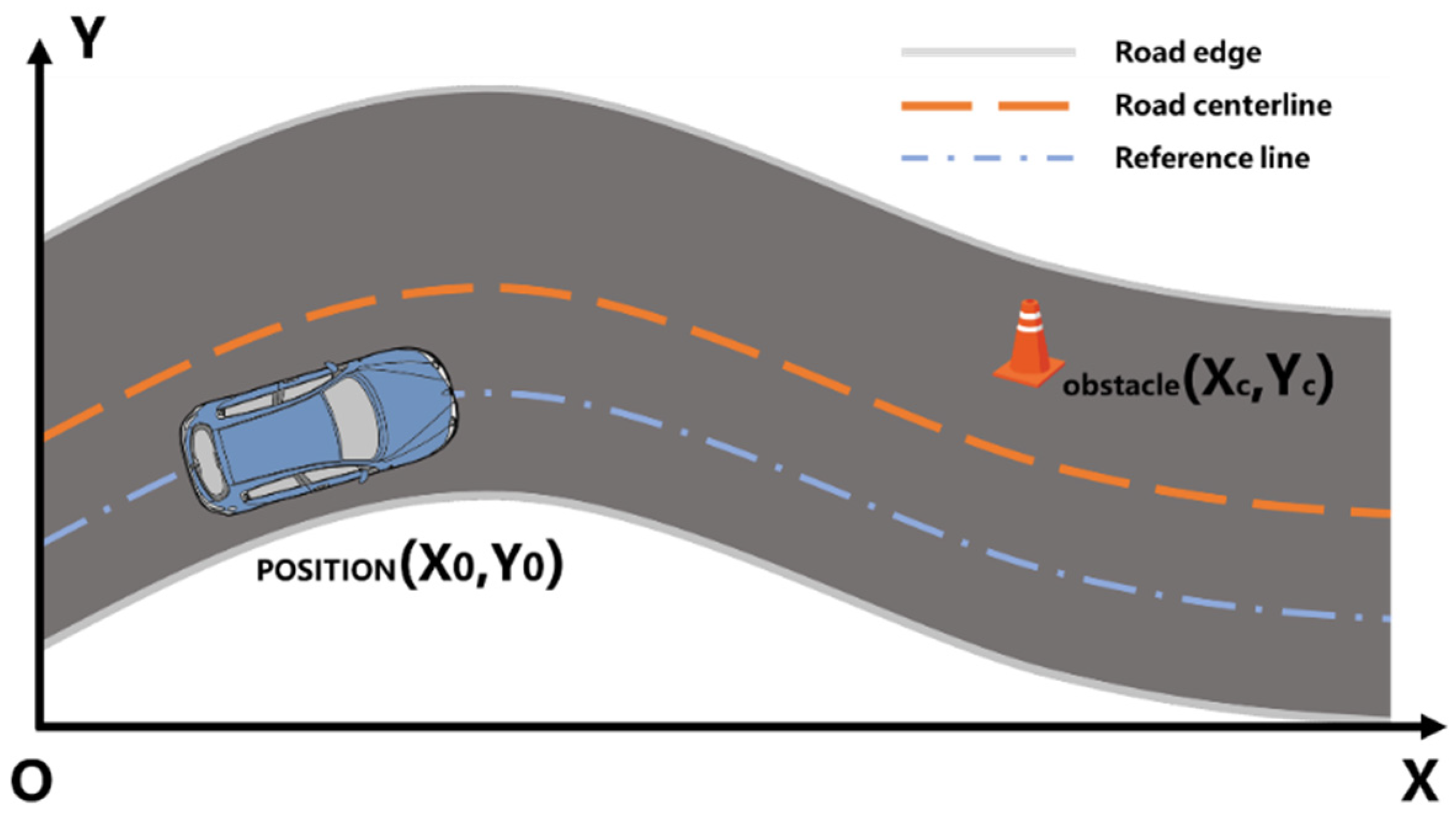
2.1. Problem Description and Basic Assumptions

Consider the driving scenario shown in Figure 1, where the vehicle is expected to drive along the center line of the current lane (i.e., the reference line in Figure 1). A human driver will adjust the distance between the vehicle and the reference line during the driving process with his perception and experience, and an AV will be expected to control the vehicle in the same manner as a human driver when performing a same driving task. A Cartesian coordinate system can be established with reference to the orientation of the road to specify the vehicle’s position $\left(X_0, Y_0\right)$. However, it is complicated to evaluate the deviation of the vehicle from the reference line in the Cartesian coordinate system, and it is not well adapted for curved roads.

Because the reference line tends to be generated along the centerline of the road, the reference line is differentiable in most roads. Then, the tangential and normal directions of any point on the reference line can be calculated, and a Frenet frame as shown in Figure 2 can be constructed. For each planning period, there will be a Frenet coordinate origin, and there will be vehicle coordinates and obstacle coordinates in the Frenet frame corresponding to the Cartesian coordinate system. Taking the scenario in Figure 2 as an example, the Frenet coordinates of the obstacle are $\left(s_5, d_2\right)$ at this point. When the vehicle moves along the green trajectory in Figure 2, a set of Frenet coordinates consisting of an arc length $s$ and a normal offset length $d$ corresponding to their Cartesian coordinates exists at each moment. These two coordinate systems will be used to describe the motion state of the AV in this paper.

Assuming that the road edge is continuously smooth, and its centerline is accordingly smooth, AVs are expected to follow the reference line in most cases. It is necessary to temporarily deviate from the reference line for the AV when there are obstacles or other vehicles on the reference line. The task of the motion planning is to find the safest and most comfortable trajectory for the AV within a planning period.

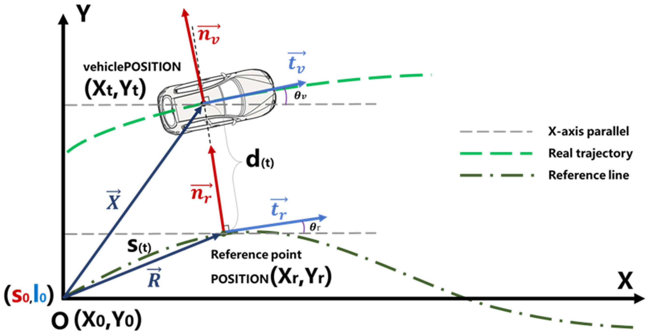
2.2. Coordinates Transformation and the Reference Line Generation

The trajectory of an AV can more easily be represented in the Frenet frame due to the irregular road structure, whereas the inputs and outputs of the motion planning need to be transformed into Cartesian coordinates. Moreover, the process of calculating the distance between two points on the trajectory is indispensable during the trajectory checking. For each set of coordinates in the Frenet frame, it is necessary to define the transformation between it and the corresponding coordinates in the Cartesian coordinate system.

As shown in Figure 3, assuming that the Cartesian coordinates $\left(X_t, Y_t\right)$ of a point at moment $t$ on the real trajectory of the AV are known, there exists a reference point $\left(X_r, Y_r\right)$ on the s-axis of the Frenet frame that minimizes the distance from the point $\left(X_r, Y_r\right)$ to the point $\left(X_t, Y_t\right)$. Then, the curve length from the point $\left(X_r, Y_r\right)$ to the coordinate origin in the Frenet frame is the s-coordinate of the AV at time $t$, and the distance length from the point $\left(X_r, Y_r\right)$ to the point $\left(X_t, Y_t\right)$ is the l-coordinate of the AV at time $t$. Therefore, the Frenet coordinates of the vehicle at moment $t$ are $\left(s_t, l_t\right)$. The value of $l_t$ can be calculated from Equations (1) and (2).

$$\overrightarrow{X}=\overrightarrow{R}+d_t\overrightarrow{n_r}$$

(1)

$$l_t=sign({\rho }_l)d_t=sign({\rho }_l)\sqrt{{\left(X_t-X_r\right)}^2+{\left(Y_t-Y_r\right)}^2}$$

(2)

where $\overrightarrow{X}$ and $\overrightarrow{R}$ are vectors of the coordinate origin pointing to the vehicle position and the reference point, respectively; $sign$ represents a symbolic function, which can only take the value of 1 or −1; ${\rho }_l$ is the parameter to determine the positive or negative of the $l$ coordinate, which can be calculated from Equation (3).

$${\rho }_l=\left(Y_t-Y_r\right)\cos {\theta }_r-\left(X_t-X_r\right)sin{\theta }_r$$

(3)

where ${\theta }_r$ is the heading angle of the reference point at moment $t$.

When the Frenet coordinates $\left(s_t, d_t\right)$ of the AV at moment $t$ are known, the Cartesian coordinates of the AV at that time can be found with the help of the heading angle of the reference line. As shown in Figure 3, the unit tangent vector $\overrightarrow{t_r}$ and the unit normal vector $\overrightarrow{n_r}$ can be found at all points on the reference line. The angle ${\theta }_r$ between the $\overrightarrow{t_r}$ and the parallel line of the x-axis in the Cartesian coordinate system is defined as the heading angle of that point, and $\overrightarrow{n_r}$ is in the same direction as the d-axis of the Frenet frame at this moment. The coordinates in the Cartesian coordinate system of the AV at moment $t$ can be calculated by Equation (4).

$$\left(X_t, Y_t\right)=\left(X_r, Y_r\right)+d_t\overrightarrow{n_r}$$

(4)

The premise of the above transformation process is that the points on the s-axis in the Frenet frame are known. AVs usually undertake global path planning based on the HD map according to their origin and destination. Then the lane center lines at each stage is spliced to obtain the reference line by referring to the road information given by the global path planning. From the perspective of vehicle dynamics and comfort, the reference line must not have any curvature interruption. The discrete original waypoints obtained on the HD map are interpolated by applying the cubic spline curve to obtain the reference line that matches the human driver’s driving habits. The reference line is usually used as the s-axis of the Frenet frame in the motion planning process.

The s-coordinates in the Frenet frame are expected to be mapped to the Cartesian coordinate system. The path consisting of the original waypoints is sampled uniformly, and its cumulative length is expressed as $S_i$. The reference line is parameterized with $S_i$ as the independent variable. The coordinates $\left(X_{ri}, Y_{ri}\right)$ of the reference line are transformed into functions of $S_i$, i.e., $X_{ri}=f_x\left(S_i\right)$, and $Y_{ri}=f_y\left(S_i\right)$, respectively. Taking the process of interpolation of ($S_i$, $X_{ri}$) as an example, the process of cubic spline interpolation is shown in Equations (5)–(9).

$${\alpha }_i=X_{ri}$$

(5)

$${\gamma }_i=\frac{m_i}{2}$$

(6)

$${\beta }_i=\frac{{\alpha }_{i+1}-{\alpha }_i}{{\alpha }_i}-\frac{h_i}{3}\left({\gamma }_{i+1}+2{\gamma }_i\right)$$

(7)

$${\delta }_i=\frac{{\gamma }_{i+1}-{\gamma }_i}{3h_i}$$

(8)

$$f_x\left(S_i\right)={\alpha }_i+{\beta }_i\left(S-S_i\right)+{\gamma }_i{\left(S-S_i\right)}^2+{\delta }_i{\left(S-S_i\right)}^3$$

(9)

where $h_i=S_{i+1}-S_i$ represents step size; $m_i$ is a quadratic differential value that satisfies the condition $h_i{m}_i+2\left(h_i+h_{i+1}\right)m_{i+1}+h_{i+1}{m}_{i+2}=6\left[\frac{X_{ri+2}-X_{ri+1}}{h_{i+1}}-\frac{X_{ri+1}-X_{ri}}{h_i}\right]$. The value of $m_i$ can be solved by applying the Not-A-Knot boundary condition to these equations.

After the cubic spline interpolations, the information of all the sampling points on the pre-selected driving centerline can be obtained in the Frenet frame and the Cartesian coordinate system. A usable reference line can be obtained. For the convenience of presentation, the longitudinal and lateral positions mentioned in this paper represent the coordinates in the Frenet frame. The vehicle positions in the Cartesian coordinate system will be expressed in x- and y-coordinates.

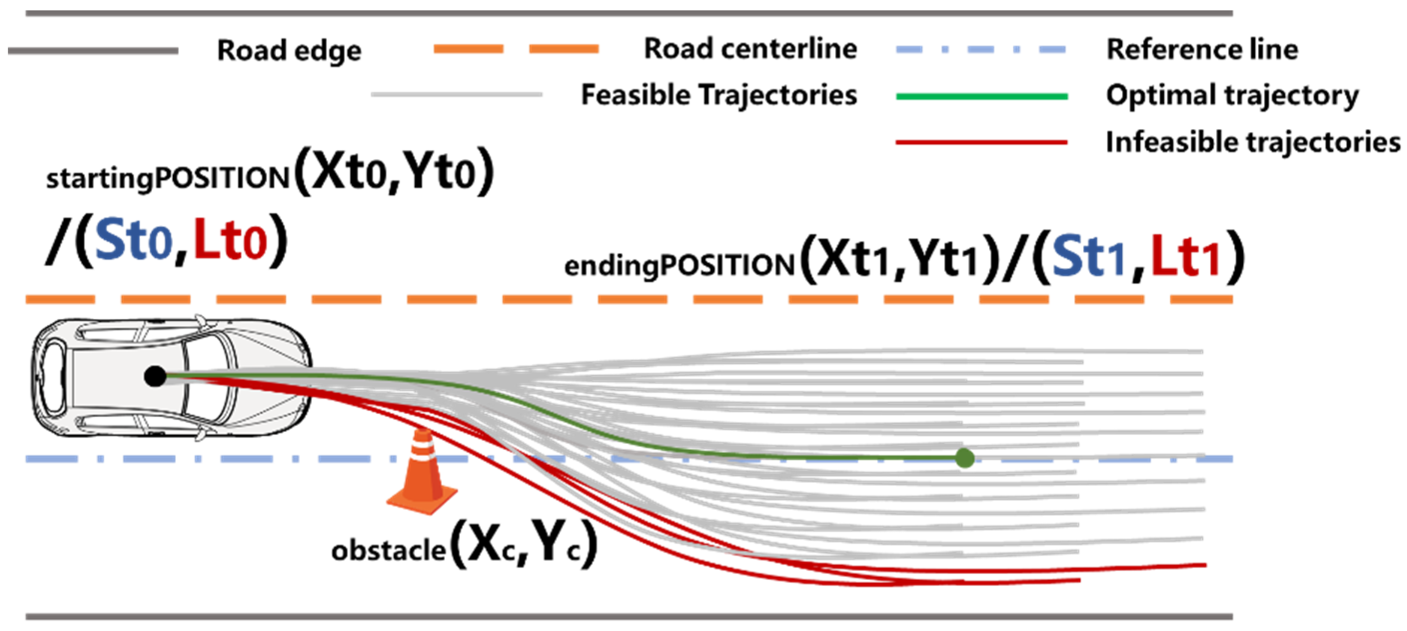
2.3. Trajectories Generation

In this section, the optional trajectories of the AV are described by mathematical equations. Safety and comfort are especially important during the motion of an AV. The degree of jerking is used to evaluate the comfort level when generating a trajectory, i.e., the derivative of the vehicle acceleration. The polynomial can generate smooth curves while imposing a series of constraints on the curves, which is very suitable for solving the problem of trajectory generation. The trajectories in a time-varying and two-dimensional space need to satisfy multiple constraints from the lateral and longitudinal motion in the Frenet frame. Because the accuracy and speed of the solution can be affected when the order of the polynomial is too high, the lateral and longitudinal motions of the vehicle are described as polynomials of the vehicle state concerning time.

For the lateral motion of the vehicle, the lateral states of vehicles in a planning period can be defined as $\left\{d_{t0},\dot{ d_{t0}},\ddot{ d_{t0}}, d_{t1},\dot{ d_{t1}},\ddot{ d_{t1}}\right\}$, where $d_{t0}$ and $d_{t1}$ represent the starting lateral position and the ending lateral position of the vehicle, respectively. $\dot{d_{t0}}$ and $\dot{d_{t1}}$ denote the starting lateral velocity and the ending lateral speed of the vehicle, respectively. $\ddot{d_{t0}}$ and $\ddot{d_{t1}}$ represent the starting lateral acceleration and the ending lateral acceleration of the vehicle, respectively. The motion planning problem can be transformed into a constrained functional extremum solution problem as shown in Equation (10).

$$\begin{gathered} find f_{lateral}\left(t\right) that minimizes {{\displaystyle \int }}_{t_0}^{t_1}{\stackrel{\dots }{(f_{lateral})}}^{2}dt \\ subject to \left\{\begin{array}{c} f_{lateral}\left(t0\right)=d_{t0}, f_{lateral}\left(t1\right)=d_{t1} \\ \dot{ f_{lateral}\left(t0\right)}=\dot{d_{t0}}, \dot{ f_{lateral}\left(t1\right)}=\dot{d_{t1}}\\ \ddot{ f_{lateral}\left(t0\right)}=\ddot{d_{t0}}, \ddot{ f_{lateral} \left(t1\right)}=\ddot{d_{t1}} \end{array}\right\} \end{gathered}$$

(10)

where $f_{lateral}\left(t\right)$ is the mathematical function concerning the lateral distance of the motion of the AV with respect to moment t; ${\int }_{t_0}^{t_1}{\stackrel{\dots }{(f_{lateral})}}^{2}dt$ is the integral of the square of the lateral motion jerk from $t0$ to $t1$.

Obviously $f_{lateral}\left(t\right)$ must be a continuous bounded function in $\left[t0, t1\right]$, otherwise $\stackrel{\dots }{f_{lateral}}$ would appear to be infinite and make the problem unsolvable. The quintic polynomial shown in Equation (11) is used to represent $f_{lateral}\left(t\right)$.

$$\begin{gathered} f_{lateral}\left(t\right)=a_{d0}+a_{d1}t+a_{d2}{t}^2+a_{d3}{t}^3+a_{d4}{t}^4+a_{d5}{t}^5 \\ \dot{f_{lateral}\left(t\right)}=a_{d1}+2a_{d2}t+3a_{d3}{t}^2+4a_{d4}{t}^3+5a_{d5}{t}^4 \\ \ddot{f_{lateral}\left(t\right)}=2a_{d2}+6a_{d3}t+12a_{d4}{t}^2+20a_{d5}{t}^3 \\ subject to \left\{\begin{array}{c} f_{lateral}\left(t0\right)=d_{t0}, f_{lateral}\left(t1\right)=d_{t1} \\ \dot{ f_{lateral}\left(t0\right)}=\dot{d_{t0}}, \dot{ f_{lateral}\left(t1\right)}=\dot{d_{t1}}\\ \ddot{ f_{lateral}\left(t0\right)}=\ddot{d_{t0}}, \ddot{ f_{lateral}\left(t1\right)}=\ddot{d_{t1}} \end{array}\right\} \end{gathered}$$

(11)

where $a_{d0}$, $a_{d1}$, $a_{d2}$, $a_{d3}$, $a_{d4}$, and $a_{d5}$ are the parameters of the quintic polynomial, which can be solved by substituting the constraints to obtain the values of each parameter, as shown in Equations (12)–(17). For convenience, assume that $t1-t0=\tau$.

$$a_{d0}=d_{t0}$$

(12)

$$a_{d1}=\dot{d_{t0}}$$

(13)

$$a_{d2}=\frac{\ddot{d_{t0}}}{2}$$

(14)

$$a_{d3}=\frac{-\left(20d_{t0}-20d_{t1}+12\tau \dot{d_{t0}}+8\tau \dot{d_{t1}}+3{\tau }^2\ddot{d_{t0}}-{\tau }^2\ddot{d_{t1}}\right)}{2{\tau }^3}$$

(15)

$$a_{d4}=\frac{30d_{t0}-30d_{t1}+16\tau \dot{d_{t0}}+14\tau \dot{d_{t1}}+3{\tau }^2\ddot{d_{t0}}-{\tau }^2\ddot{d_{t1}}}{2{\tau }^4}$$

(16)

$$a_{d5}=\frac{-\left(12d_{t0}-12d_{t1}+6\tau \dot{d_{t0}}+6\tau \dot{d_{t1}}+{\tau }^2\ddot{d_{t0}}-{\tau }^2\ddot{d_{t1}}\right)}{2{\tau }^5}$$

(17)

It is important to note that $f_{lateral}\left(t\right)$ is not a standard planning process because the AV cannot move only in the lateral direction with moment $t$. Therefore $f_{lateral}\left(t\right)$ can only guarantee the smoothness and comfort of the trajectories in the lateral direction. It is also necessary to describe and constrain the longitudinal motion.

Similar to the lateral motion planning, the longitudinal motion planning problem can be transformed into $find f_{longitudinal}\left(t\right) that minimizes {\int }_{t_0}^{t_1}{\stackrel{\dots }{(f_{longitudinal})}}^{2}dt$. It is feasible to describe longitudinal motion in the same manner, but the driving strategies sometimes affect the vehicle’s motion constraints. In the usual case, the AV is expected to arrive at a specified location within time $\tau$ to execute the order of the upper system. The constraints of longitudinal motion in this case are like those on lateral motion, and a quintic polynomial as shown in Equation (18) is used to represent $f_{longitudinal}\left(t\right)$ in this case.

$$\begin{gathered} f_{longitudinal}\left(t\right)=a_{s0}+a_{s1}t+a_{s2}{t}^2+a_{s3}{t}^3+a_{s4}{t}^4+a_{s5}{t}^5 \\ \dot{f_{longitudinal}\left(t\right)}=a_{s1}+2a_{s2}t+3a_{s3}{t}^2+4a_{s4}{t}^3+5a_{s5}{t}^4 \\ \ddot{f_{longitudinal}\left(t\right)}=2a_{s2}+6a_{s3}t+12a_{s4}{t}^2+20a_{s5}{t}^3 \\ subject to \left\{\begin{array}{c} f_{longitudinal}\left(t0\right)=s_{t0}, f_{longitudinal}\left(t1\right)=s_{t1} \\ \dot{ f_{longitudinal}\left(t0\right)}=\dot{s_{t0}}, \dot{ f_{longitudinal}\left(t1\right)}=\dot{s_{t1}}\\ \ddot{ f_{longitudinal}\left(t0\right)}=\ddot{s_{t0}}, \ddot{ f_{longitudinal}\left(t1\right)}=\ddot{s_{t1}} \end{array}\right\} \end{gathered}$$

(18)

where $s_{t0}$ and $s_{t1}$ represent the starting longitudinal position and the ending longitudinal position of the vehicle motion, respectively; $\dot{s_{t0}}$ and $\dot{s_{t1}}$ represent the starting longitudinal speed and the ending longitudinal speed of the vehicle, respectively; $\ddot{s_{t0}}$ and $\ddot{s_{t1}}$ represent the starting longitudinal acceleration and the ending longitudinal acceleration of the AV, respectively; and $a_{s0}$, $a_{s1}$, $a_{s2}$, $a_{s3}$, $a_{s4}$, and $a_{s5}$ are the parameters of the quintic polynomial, which can be solved by substituting the constraints to obtain the values of each parameter, as shown in Equations (19)–(24).

$$a_{s0}=s_{t0}$$

(19)

$$a_{s1}=\dot{s_{t0}}$$

(20)

$$a_{s2}=\frac{\ddot{s_{t0}}}{2}$$

(21)

$$a_{s3}=\frac{-\left(20s_{t0}-20s_{t1}+12\tau \dot{s_{t0}}+8\tau \dot{s_{t1}}+3{\tau }^2\ddot{s_{t0}}-{\tau }^2\ddot{s_{t1}}\right)}{2{\tau }^3}$$

(22)

$$a_{s4}=\frac{30s_{t0}-30s_{t1}+16\tau \dot{s_{t0}}+14\tau \dot{s_{t1}}+3{\tau }^2\ddot{s_{t0}}-{\tau }^2\ddot{s_{t1}}}{2{\tau }^4}$$

(23)

$$a_{s5}=\frac{-\left(12s_{t0}-12s_{t1}+6\tau \dot{s_{t0}}+6\tau \dot{s_{t1}}+{\tau }^2\ddot{s_{t0}}-{\tau }^2\ddot{s_{t1}}\right)}{2{\tau }^5}$$

(24)

In addition, there are cases when we want the AV to maintain a constant speed while ensuring safety and smoothness of trajectories, and its ending position within a planning period is not considered. Then, the number of constraints is 5 (i.e., starting longitudinal position $s_{t0}$, starting longitudinal speed $\dot{s_{t0}}$, starting longitudinal acceleration $\ddot{s_{t0}}$, ending longitudinal speed $\dot{ s_{t1}}$, and ending longitudinal acceleration $\ddot{s_{t1}}$). A quadratic polynomial, as shown in Equation (25), is used to represent the $f_{longitudinal}\left(t\right)$ for the velocity maintenance case.

$$\begin{gathered} f_{longitudinal}\left(t\right)=b_{s0}+b_{s1}t+b_{s2}{t}^2+b_{s3}{t}^3+b_{s4}{t}^4 \\ \dot{f_{longitudinal}\left(t\right)}=b_{s1}+2b_{s2}t+3b_{s3}{t}^2+4b_{s4}{t}^3 \\ \ddot{f_{longitudinal}\left(t\right)}=2b_{s2}+6b_{s3}t+12b_{s4}{t}^2 \\ subject to \left\{\begin{array}{c} f_{longitudinal}\left(t0\right)=s_{t0}\\ \dot{ f_{longitudinal}\left(t0\right)}=\dot{s_{t0}}, \dot{ f_{longitudinal}\left(t1\right)}=\dot{s_{t1}}\\ \ddot{ f_{longitudinal}\left(t0\right)}=\ddot{s_{t0}}, \ddot{ f_{longitudinal}\left(t1\right)}=\ddot{s_{t1}} \end{array}\right\} \end{gathered}$$

(25)

where $b_{s0}$, $b_{s1}$, $b_{s2}$, $b_{s3}$, and $b_{s4}$ are the parameters of the quintic polynomial, which can be solved by substituting the constraints to obtain the values of each parameter, as shown in Equations (26)–(30).

$$b_{s0}=s_{t0}$$

(26)

$$b_{s1}=\dot{s_{t0}}$$

(27)

$$b_{s2}=\frac{\ddot{s_{t0}}}{2}$$

(28)

$$b_{s3}=\frac{-\left(3s_{t0}-3s_{t1}+2\tau \ddot{s_{t0}}+\tau \ddot{s_{t1}}\right)}{3{\tau }^2}$$

(29)

$$b_{s4}=\frac{2s_{t0}-2s_{t1}+\tau \dot{s_{t0}}+\tau \dot{s_{t1}}}{4{\tau }^3}$$

(30)

After determining $f_{lateral}\left(t\right)$ and $f_{longitudinal}\left(t\right)$, a series of smooth trajectories can be obtained between the starting position and all optional ending positions of the AV in a motion planning period.

2.4. Optimal Trajectories Searching Based on the Cost Function

In a motion planning period, optional trajectories are obtained after selecting an optional ending position. The performance of the trajectories is evaluated by defining the cost function; a series of costs and their weights are defined as shown in

Table 1. Cost definitions of the trajectories.

Cost	Weight
$C_{J_d}={{\displaystyle \int }}_{t0}^{t1}({\stackrel{\dots }{f_{lateral}\left(t\right))}}^{2}dt$	$w_{J_d}$
$C_{J_s}={{\displaystyle \int }}_{t0}^{t1}({\stackrel{\dots }{f_{longitudinal}\left(t\right))}}^{2}dt$	$w_{J_s}$
$C_t=t1-t0$	$w_t$
$C_{offset}={{\displaystyle \int }}_{t0}^{t1}{(f_{lateral}\left(t\right))}^{2}dt$	$w_o$
$C_{velocity}=\dot{(f_{longitudinal}\left(t1\right)}-V_{target}{)}^2$	$w_v$
$C_{collision}=\frac{1}{{\int }_{t0}^{t1}{(distanc{e}_{x-obstacle})}^{2}dt}$	$w_c$

. In consideration of human comfort, we consider lateral and longitudinal jerking, and the jerking is used to evaluate the comfort level of trajectories when the AV is moving, i.e., the derivative of the AV’s acceleration. In consideration of efficiency, we also penalize longer trajectories that take more time to assess. In addition, shorter trajectories can sometimes lead to higher mobility. In general, we expect the AV to follow the reference line, so we penalize deviations from the reference line. For safety, we introduce the reciprocal of the cumulative distance between the trajectory and the obstacles to avoid risky behaviors. The weights of the cost function can be adjusted according to different scenarios. Equal weights are used in this study, which means each indicator is considered to be equally important.

As shown in Table 1, $C_{J_d}$ and $C_{J_s}$ represent the jerk cost of lateral motion and the jerk cost of longitudinal motion of the AV. $C_{offset}$ represents the degree of offset of the AV from the reference line. $C_{velocity}$ represents the deviation between the planning speed and the desired speed. $distanc{e}_{x-obstacle}$ represents the minimum distance between the AV and the obstacles.$C_{collision}$ represents the cost of a collision between the AV and the static or dynamic obstacles.

In an automated vehicle system, these costs are calculated in the form of discrete sampling points. Then, all the integral operations are replaced by cumulative summation. Supposing that there are $n$ sampling moments in the planning period $\left[t0, t1\right]$, the cost function of a trajectory is expressed as Equation (31).

$$\begin{gathered} C_{total}=w_{J_d}{C}_{J_d}+w_{J_s}{C}_{J_s}+w_t{C}_t+w_o{C}_{offset}+w_v{C}_{velocity}+w_c{C}_{collision} \\ =w_{J_d}{\displaystyle \sum }_{k=1}^n({\stackrel{\dots }{f_{lateral}\left(k\right))}}^2+w_{J_s}{\displaystyle \sum }_{k=1}^n({\stackrel{\dots }{f_{longitudinal}\left(k\right))}}^2+w_t\left(t1-t0\right) \\ +w_o{\displaystyle \sum }_{k=1}^n{(f_{lateral}\left(k\right))}^2+w_v\dot{(f_{longitudinal}\left(t1\right)}-V_{target}{)}^2 \\ +w_c\frac{1}{{\sum }_{k=1}^n{(distanc{e}_{x\left(k\right)-obstacles})}^2} \end{gathered}$$

(31)

where $C_{total}$ represents the total cost of an optional trajectory. Therefore, the trajectory with the lowest cost can be found by calculating the cost of all trajectories in turn.

2.5. Final Path Selection

After the optimal trajectory searching process is completed, all trajectories are sorted in order of cost from minimum to maximum, and pass through the trajectory checking process in this order.

As shown in Figure 4, assuming that there are $m$ sets of different combinations of lateral ending position $d_{t1}$, ending time $t1$, and ending speed $\dot{s_{t1}}$ in the sampling space of motion planning at moment $t0$, there are $m$ optional ending positions in the sampling space of the AV in this motion planning period, which means that there are $m$ optional trajectories. The cost of $m$ trajectories is calculated according to Equation (31). These trajectories are sorted in order of cost from minimum to maximum. From the perspective of safety and comfort, these trajectories need to be checked by the maximum velocity, maximum acceleration, maximum curvature, and collision to obtain a preliminary total of $m^{\prime }$ trajectories satisfying those physical properties. The first trajectory that passes the check in this sorted set of trajectories is the final path selection for the current period. The AV then moves along this path until the start of the next planning period.

When the next planning period starts, the AV’s motion state is considered as the initial state of the AV for the next period and the above process is repeated. The AV obtains the complete path through continuous loop iteration.

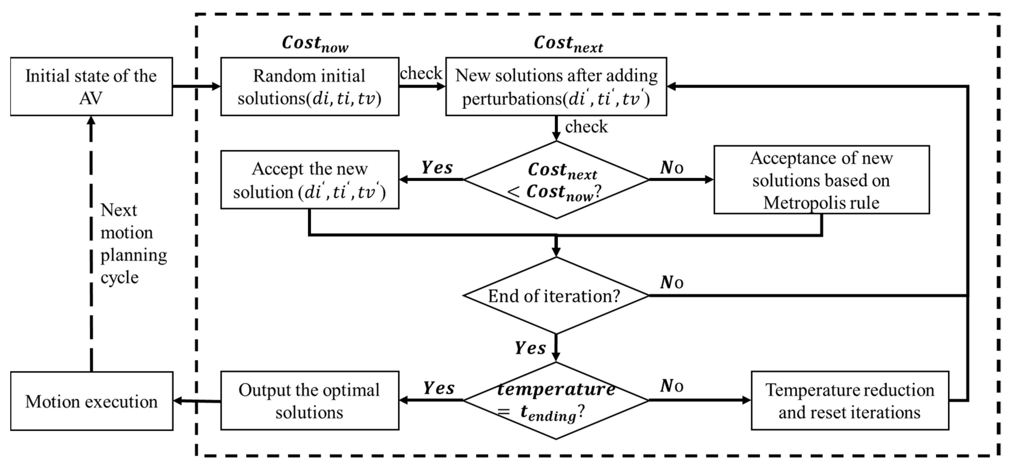
3. Improved Optimal Trajectory Searching Process Based on SAA

After determining the sampling space, it is common practice to compute all the trajectories and to examine the trajectories [22,23,31]. The costs of all trajectories in a typical sampling space are shown in Figure 5, where different trajectories are distinguished by the lateral and longitudinal coordinates of the Frenet frame at the ending position of the AV during the motion planning period. Assuming that the initial position of the AV is located on the reference line, the costs of different trajectories without obstacles are shown in Figure 5a, where the x-axis represents the longitudinal positions of the ending points of the trajectories, the y-axis represents the transverse positions of the ending points of the trajectories, and the z-axis represents the costs. Figure 5b shows the contour projection based on Figure 5a. It can be observed that the costs show an obvious axisymmetric regularity about the reference line. High-cost trajectories end off of the reference line, whereas low-cost trajectories tend to end on the reference line. This conclusion can also be verified in theory through the cost calculation function in Equation (31), because we penalize the degree of reference line offset and the lateral jerk. In addition, the other penalty terms also show the same symmetry regularity along the reference line. Based on this regularity, it can be speculated that when there are obstacles in the sampling space, the cost distribution of the trajectories close to the obstacles will produce obvious fluctuations.

To verify this speculation, two scenarios with the existence of static obstacles were performed. It is assumed that the starting position of the AV is located on the reference line, and the AV drives at $40 \mathrm{k}\mathrm{m}/\mathrm{h}$ along the reference line direction. The costs of different trajectories with a static obstacle placed at $35 \mathrm{m}$ along the reference line direction directly in front of the AV is shown in Figure 6a, while the x-axis indicates the longitudinal positions of the ending points of the trajectory, the y-axis indicates the lateral positions of the ending points of the trajectory, and the z-axis indicates the costs. Figure 6b shows the contour projection of the costs. It can be observed that when there is a static obstacle on the reference line, the costs of all trajectories increase significantly along the reference line, i.e., the lateral ending position at $0 \mathrm{m}$. Figure 6c,d show the costs of different trajectories when the static obstacle is placed $35 \mathrm{m}$ in front of the adjacent left lane. In this case, the costs are similar to the previous static obstacle case. However, the fluctuation is not obvious for longer trajectories, which is because the arc of long trajectories circumvents the obstacles closer to the starting point. Based on the above verification, it can be determined that there is a certain regularity in the costs of the trajectories. The costs show an axisymmetric regularity when the starting position of the AV is located on the reference line, and the existence of obstacles will lead to an increase in the costs of the nearby trajectories.

Combining this symmetry regularity, we modify the cost function of the AV to ensure that it better follows the driving habits of human drivers and has better safety and comfort. Due to traffic rules and driving habits, human drivers in China tend to pass or avoid other vehicles from the left side. Therefore, we hope that the trajectory on the left side will be less costly when there are feasible trajectories on both sides of the reference line. The cost is modified as shown in Equation (32).

$$C_{final}=\{\begin{array}{ll}{C}_{total}-sign\left(d_{t1}\right)\epsilon & d_{t1}\ne 0\\ C_{total}-\epsilon & d_{t1}=0\end{array}$$

(32)

where $C_{final}$ represents the modified cost; $\epsilon$ represents a very small non-zero positive number; $sign$ represents the sign function; $d_{t1}$ represents the distance between the ending position of the trajectory and the reference line.

Therefore, the cost of all trajectories in the sampling space of a planning period forms a nonconvex space. The global optimal solution is often found by calculating the costs of all trajectories after sampling to prevent finding a locally optimal solution. We use the SAA to replace the process of calculating the cost, which refines the sampling interval with a fixed number of samples. The process of finding the optimal trajectory by SAA is contained in the dashed box in Figure 7. The variables in the optional solution are the lateral ending position of the trajectory ($di$), the planning time during the period ($ti$), and the longitudinal ending speed of the trajectory ($tv$). The optimal combination of variables is obtained by the searching process, including the inner isothermal layer and the probability adjustment of the outer layer with constant cooling. In addition, the corresponding trajectory is checked immediately after each set of solutions and generated to ensure comfort and safety. A new set of solutions is generated if the check does not pass. The computational effort of trajectory generation and cost calculation will be greatly reduced by setting a reasonable iteration number and temperature coefficients. The key part of SAA is the Metropolis acceptance rule. We avoid falling into a local optimum by utilizing the property of accepting poorer solutions with a certain probability described mathematically, as shown in Equation (33).

$$P=\{\begin{array}{ll}1,& Cos{t}_{next}<Cos{t}_{now}\\ e^{\frac{-\left(Cos{t}_{next}-Cos{t}_{now}\right)}{kT}},& Cos{t}_{next}\ge Cos{t}_{now} \end{array}$$

(33)

where $P$ represents the probability of accepting the new solution; $Cos{t}_{now}$ and $Cos{t}_{next}$ represent the costs of the trajectories corresponding to the current solution and the new solution, respectively; $k$ is the temperature dropping rate, and the value is between 0 and 1; $T$ represents the system temperature.

4. Numerical Experiments

In this section, the performance of the proposed motion planning method is analyzed to demonstrate the effectiveness in several typical traffic scenarios on a three-lane road, including maintaining speed, lane changing, and car following. It was assumed that decisions of the AV were provided from the behavior planning layer, and all traffic participants were going in the same direction. In these experiments, the lateral and longitudinal motions of the AV were given by the quadratic or quintic polynomials described in Equations (11), (18) and (25). By sampling the road environment ahead, a series of optional motion trajectories consisting of different lateral and longitudinal motions are obtained. The traversal method and the SAA-based method proposed in this study were applied to search for the optimal trajectory among these optional trajectories, respectively. In each planning period, the AV followed the optimal path that was searched for and checked. The state of the AV at the end of a planning period was inherited as the initial state of the next period, and we obtained the global driving performance of the AV by cycling through this process.

We compared the traversal method [22,23,31] and the improved method based on SAA under the same environment and parameter settings, and analyzed the computational effort, motion planning performance, and driving comfort.

4.1. Scenario and Parameter Settings

The AV was placed in a three-lane urban road scenario. The whole road was connected by $10$ original waypoints according to the cubic spline curve interpolation method in this paper. The rough length of the road was $500 \mathrm{m}$, but there were curves within the first $200 \mathrm{m}$, and the width of each lane was $3.6 \mathrm{m}$. Three vehicles driven by human drivers at different speeds drove around the AV at the beginning of the simulation, and parameters of all vehicles were set as shown in

Table 2. Parameters of the vehicles.

Vehicle Parameters	Value	Unit
Vehicle width (for all vehicles)	2.0	m
Vehicle length (for all vehicles)	4.2	m
Collision radius of the vehicle (for all vehicles)	3.0	m
The initial position of the AV	(0, 0)	m
The initial position of the vehicles driven by human drivers	(30.0, 0.0), (80.0, 3.6),(15.0, −3.6)	m
The initial speed of the AV	40	km/h
The speed of the vehicles driven by human drivers	20, 30, 40	km/h

.

For convenience, we named the method that calculates the trajectory cost based on the exhaustive method, Method A, and the method based on SAA, Method B. To compare the two methods, the sampling space needed to be set with consistent settings, and the parameters of the sampling space for the AV in each motion planning period were set as shown in

Table 3. The parameters of the sampling space.

Sampling Space Parameters	Method A	Method B
Lateral position sampling range (m)	[−4.2, 4.2]	[−4.2, 4.2]
Predicted time sampling range (s)	[4, 5]	[4, 5]
Target speed sampling range (km/h)	[35, 45]	[35, 45]
Lateral position sampling interval (m)	1	0.1
Predicted time sampling interval (s)	0.1	0.1
Target speed sampling interval (km/h)	5	5
Planning period length (s)	0.1	0.1

.

For Method A, the number of generated trajectories and costs that needed to be calculated increases exponentially along with the increase in the number of sampling points, which could not satisfy the requirement of trajectory computation. Therefore, we limited the number of lateral sampling points in Method A to improve the calculation performance.

For Method B, the parameters of SAA were set as shown in

Table 4. Parameters of SAA.

Parameters of SAA	Values
Initial temperature (°C)	100
Length of Markov chain	5
Rate of temperature decrease	0.9
The temperature at which the algorithm stops (°C)	3

.

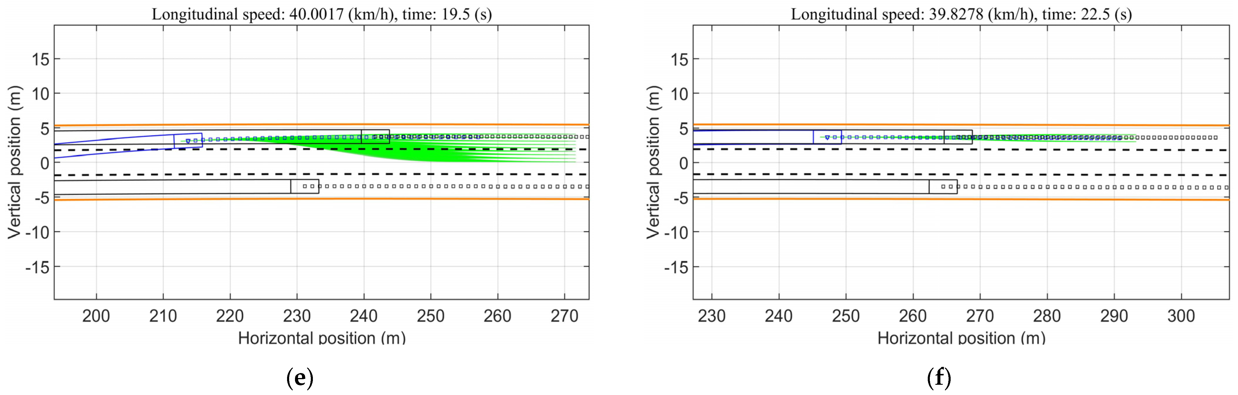
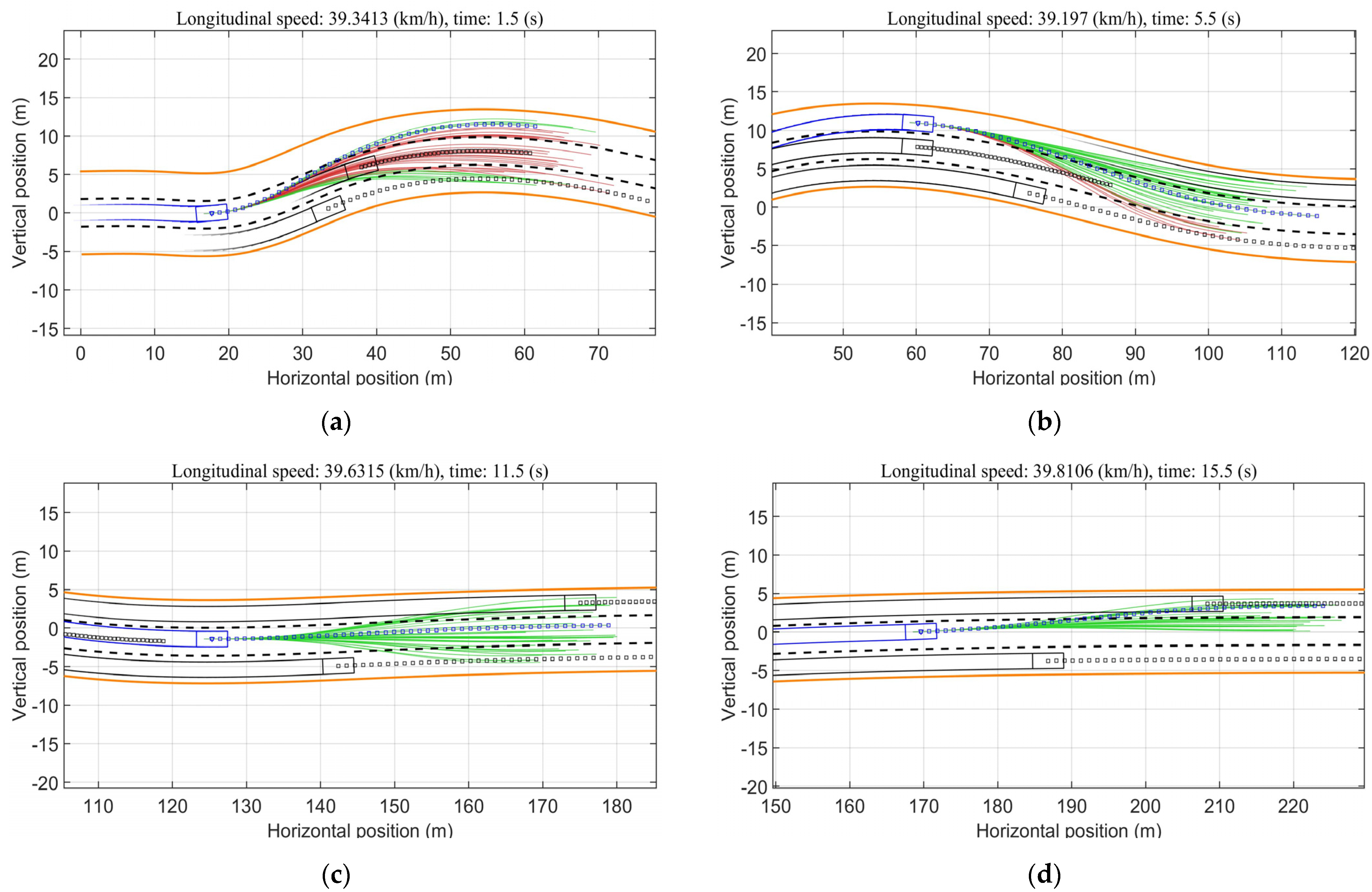
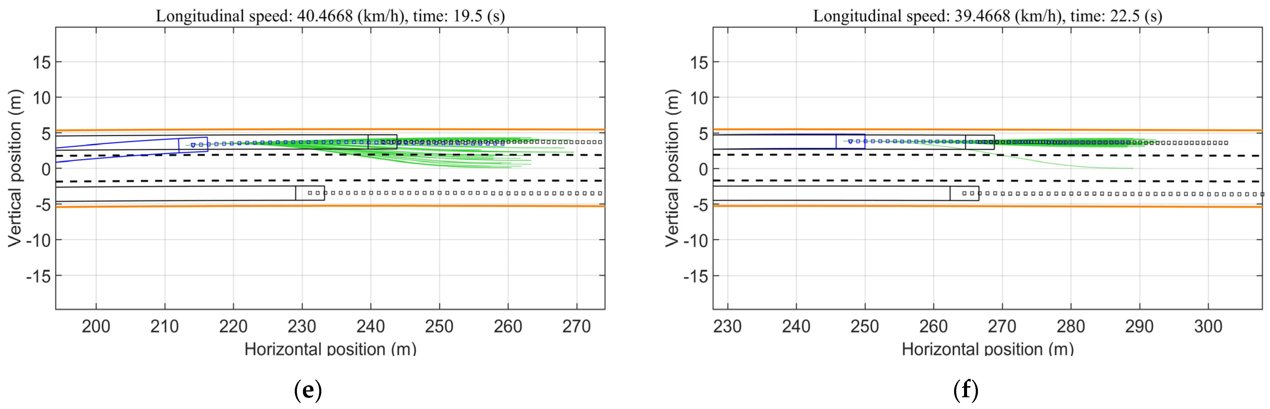
4.2. Performance of the AV with Methods A and B

All vehicles departed at the same time in the preset dynamic scenario. The AV followed the maintain speed command for the first 15 s, received the command to change to the left lane after 15 s, and performed the following command after the longitudinal distance with the left obstructing vehicle was less than $25 \mathrm{m}$. The trajectory tracking module of the AV was considered to be performing under ideal operating conditions. We tested the methods on a computer with an AMD Ryzen 5 3600 CPU (6-core, 3.9 GHz) and 16 GB RAM. The two experiments were run on the same computer with the same configuration, and the computing elapsed times were extremely long, and affected by plotting and data storage. The program can be simplified to meet real-time requirements in practical applications. The performance of the AV when applying Methods A and B is shown in Figure 8 and Figure 9, respectively. The blue rectangle represents the AV, and the black rectangles represent the obstructing vehicles driven by human drivers. The green and red trajectory lines represent the optional and nonoptional trajectories planned by the AV at the current moment, respectively. The series of blue trajectory points extending in front of the AV represent its selected optimal trajectory at the current moment, and similarly, the black trajectory points in front of the obstructing vehicles represent the predicted points of their motion trajectories in the future period. The traces left by each vehicle represent its real trajectory in the past.

Figure 8 shows the performance of the AV when applying Method A. The whole computation process took $5168.84 \mathrm{s}$. The decision command received in the first $15 \mathrm{s}$ was to maintain speed. As shown in Figure 8a–c, the optimal trajectories were to overtake the low-speed ($20 \mathrm{k}\mathrm{m}/\mathrm{h}$) obstructing vehicle from the left free lane when there were low-speed obstructing vehicles in both the current lane and the right lane. After overtaking the low-speed obstructing vehicle, the AV was controlled by the cost of offset from the reference line to return to the original lane and maintained the driving speed. As shown in Figure 8d,e, the AV received the decision command to change lane to the left and maintained the speed after $15 \mathrm{s}$, when the obstructing vehicle in the left lane was faster ($30 \mathrm{k}\mathrm{m}/\mathrm{h}$), and the searched optimal trajectories were to change lane to the left without overtaking the left obstructing vehicle. As shown in Figure 8f, when the distance between the AV and the obstructing vehicle in the left lane was less than $25 \mathrm{m}$, the decision command was changed to follow the vehicle, and the AV started to adjust its speed to follow the vehicle ahead.

As the searching process of Method A traversed all the sampled points, the AV calculated the costs of all the trajectories at each moment. This is evidenced by the red and green trajectories shown in Figure 8.

Figure 9 shows the performance of the AV when applying the motion planning Method B. The whole calculation process took $1538.82 \mathrm{s}$, and all the settings in this test were the same as those for the test of Method A, except for the different searching method for optimal trajectories. The motion planning performance of the AV under each decision command when applying Method B was basically the same as that when applying Method A; both methods completely avoided the moving obstructing vehicles. It is worth noting that the trajectories searched for by Method B shown in Figure 9 are significantly sparser at each moment compared to those of Method A. This means that Method B may achieve the same motion planning results as Method A with less computational effort.

The driving path of the AV in two numerical experiments over time and its two-dimensional projection are shown in Figure 10. The reference line is always defined as the centerline of the middle lane, and the two offsets that occur for the AV relative to the reference line correspond to the overtaking and lane changing processes in the experiments, respectively. The 3D path generated by Method A and Method B almost overlap, which indicates that the optimal trajectories selected by the AV at each moment are approximately the same when applying Method A and Method B.

In addition to the safety and efficiency, the comfort of the AV needs to be ensured. We extracted the velocity, acceleration, and jerking of the AV in two experiments to visualize the comfort. Figure 11a,b shows the velocity and acceleration changing process of the AV in the two experiments, respectively; the velocity changing based on Method A and Method B is almost the same. The averages of the absolute values of velocity error under Method A and Method B were $0.2580 \mathrm{m}/\mathrm{s}$ and $0.2450 \mathrm{m}/\mathrm{s}$, respectively. Method B based on SAA showed better velocity performance due to more dense sampling points. The large velocity deviations of both methods occurred during the lane changing process and at the beginning of the following process. The large changes in acceleration and jerking of the AV also occurred in these two processes. The smaller the acceleration changing rate, namely the degree of jerking, the greater comfort. Figure 11c,d shows the jerking variation of the AV in the two experiments. The AV maintained a very small degree of jerking under both Method A and Method B. The averages of the absolute values of longitudinal and lateral jerking of Method A were $0.1011 \mathrm{m}/{\mathrm{s}}^3$ and $0.1978 \mathrm{m}/{\mathrm{s}}^3$, respectively. The averages of the absolute values of longitudinal and lateral jerking of Method B were $0.1454 \mathrm{m}/{\mathrm{s}}^3$ and $0.2530 \mathrm{m}/{\mathrm{s}}^3$, respectively. These results indicate that the proposed Method B can ensure the comfort of the AV.

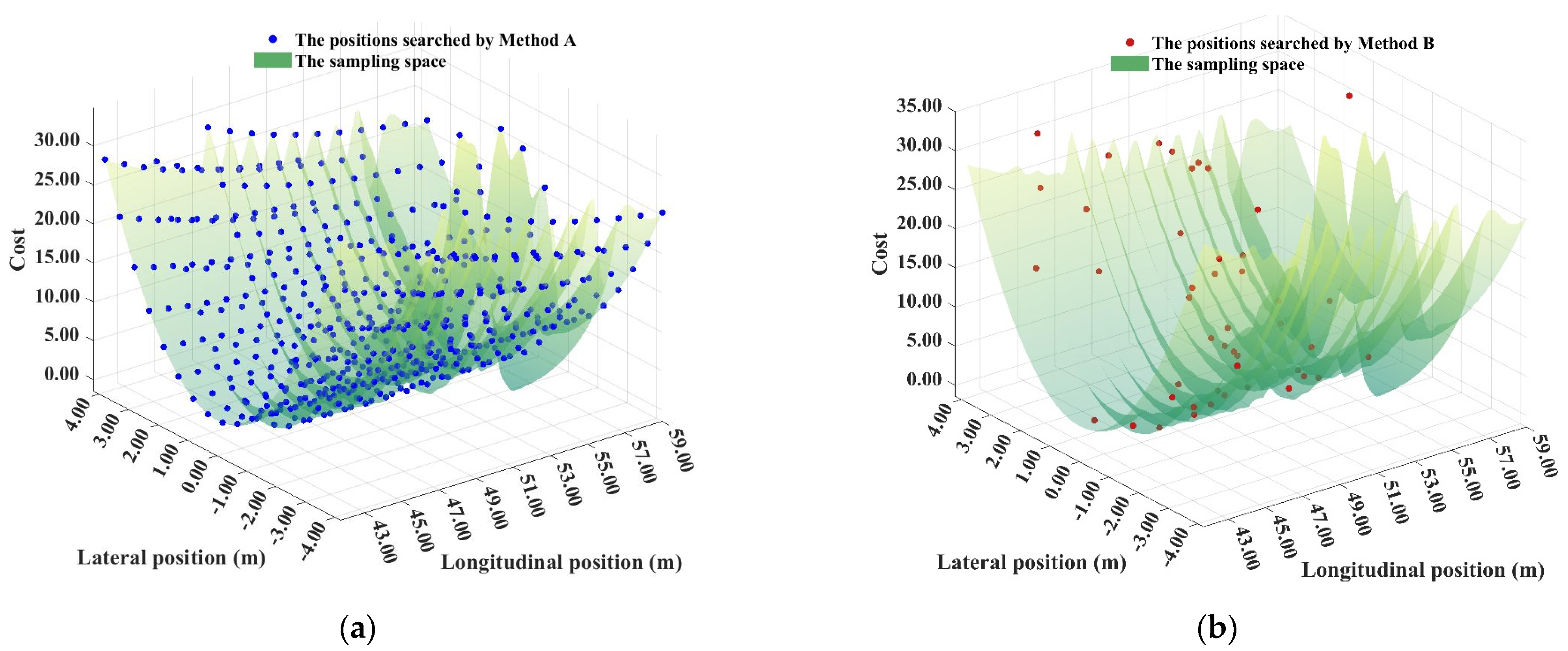
4.3. Comparison of the Efficiency of Methods A and B

Because motion planning is only one part of the process of automating an AV, it is essential to conserve the computational effort of the on-board computer. After determining that the two methods can produce nearly consistent motion planning performance for an AV in dynamic environments, we focused on the differences between the two methods in terms of computational efficiency. Figure 12a,b shows the process of searching for the optimal trajectories of the AV in the first planning period at the beginning of the simulation when applying Method A and Method B, respectively. Method A traversed the sampling space at a fixed interval and computed the costs of 561 trajectories at the moment $t=0$, taking $15.38 \mathrm{s}$. As shown for the searching process in Figure 12a, Method A was more detailed in searching the sampling space, but at the same time searched some unnecessary and costly trajectories. Method B computed the costs of 165 trajectories at the moment $t=0$, taking $5.87 \mathrm{s}$. As shown in Figure 12b, Method B is more focused on searching for less costly trajectories with the effect of SAA, and the AV performed well in dynamic traffic environments. Method B saved 62% of the planning time compared to Method A in this planning period, which proves that method B improves the efficiency of the motion planning at the moment $t=0$.

In addition, the difference between the searching time of Method A and Method B was not constant. Figure 13 shows the comparison of the searching time between the two experiments within $25 \mathrm{s}$. It can be observed that the searching time of Method A was roughly divided into three intervals, which were the speed maintaining process from $0$ to $15 \mathrm{s}$, the lane changing process from $15$ to $20 \mathrm{s}$, and the following process from $20$ to $25 \mathrm{s}$. This was because the change in the decision commands of the AV affected the sampling space. The speed maintaining decision command corresponded to the largest sampling space, covering three lanes, with the longest searching time. When the AV received the lane changing command, the sampling space was reduced to half of the original size, and the searching time was also reduced by nearly half. The sampling space of the AV was the smallest when it was performing the following command [35]. It is worth noting that the searching time of Method B was relatively stable and short because the searching method of SAA does not depend on the sampling space settings, but rather on the temperature settings to determine the searching process. The simulation process took $5168.84 \mathrm{s}$ when Method A was applied, and took $1538.82 \mathrm{s}$ when Method B was applied. Method B accelerated the whole motion planning process by $70.23\%$ compared to Method A.

5. Conclusions

Combined with the analysis of the experimental results, the following conclusions can be drawn.

• We propose a motion planning method applicable to AVs in dynamic traffic scenarios. The trajectories are solved by a polynomial in the Frenet frame, and the costs of the optional trajectories are quantified as a cost function that includes cost terms for safety, comfort, efficiency, etc. An improved optimal trajectory searching method applying SAA is proposed. The experimental results in the simulated dynamic traffic scenarios show that the method proposed in this paper is feasible and efficient.
• The process of searching for the least costly trajectory is visualized, and the axisymmetric regularity of the costs about the reference line is summarized. Based on this, the cost function is modified to make the performance of the AV more consistent with the driving behaviors of human drivers.
• Compared with the optimal trajectories searching method that traverses the sampling space, the proposed method in this paper saves 70.23% of the searching time without affecting the performance of the AV. In addition, the searching time of the proposed method shows good robustness to variations in the sampling space. This is conducive to the improvement of the motion planning adaptability of AVs in a variety of road scenarios.

In this study, we assumed that decisions of the AV were provided by the behavior planning layer. However, decision making is another challenging problem for AVs in urban scenarios. In the future, we will focus on human-like decision making and test the performance of the method in a more realistic environment.

References

1. Dijkstra, E.W. A Note on Two Problems in Connexion with Graphs. Numer. Math. 1959, 1, 269–271. [Google Scholar] [CrossRef] [Green Version]
2. Hart, P.; Nilsson, N.; Raphael, B. A Formal Basis for the Heuristic Determination of Minimum Cost Paths. IEEE Trans. Syst. Sci. Cyber. 1968, 4, 100–107. [Google Scholar] [CrossRef]
3. Ferguson, D.; Stentz, A. Using Interpolation to Improve Path Planning: The Field D* Algorithm. J. Field Robot. 2006, 23, 79–101. [Google Scholar] [CrossRef] [Green Version]
4. Kelly, A.; Nagy, B. Reactive Nonholonomic Trajectory Generation via Parametric Optimal Control. Int. J. Robot. Res. 2003, 22, 583–601. [Google Scholar] [CrossRef]
5. Claussmann, L.; Revilloud, M.; Gruyer, D.; Glaser, S. A Review of Motion Planning for Highway Autonomous Driving. IEEE Trans. Intell. Transport. Syst. 2020, 21, 1826–1848. [Google Scholar] [CrossRef] [Green Version]
6. Dolgov, D.; Thrun, S.; Montemerlo, M.; Diebel, J. Path Planning for Autonomous Vehicles in Unknown Semi-Structured Environments. Int. J. Robot. Res. 2010, 29, 485–501. [Google Scholar] [CrossRef]
7. Dolgov, D.; Thrun, S.; Montemerlo, M.; Diebel, J. Practical Search Techniques in Path Planning for Autonomous Driving. J. Field Robot. 2008, 25, 569–597. [Google Scholar]
8. Montemerlo, M.; Becker, J.; Bhat, S.; Dahlkamp, H.; Dolgov, D.; Ettinger, S.; Haehnel, D.; Hilden, T.; Hoffmann, G.; Huhnke, B.; et al. Junior: The Stanford Entry in the Urban Challenge. J. Field Robot. 2008, 25, 569–597. [Google Scholar] [CrossRef] [Green Version]
9. Karaman, S.; Frazzoli, E. Optimal Kinodynamic Motion Planning Using Incremental Sampling-Based Methods. In Proceedings of the 49th IEEE Conference on Decision and Control (CDC), Atlanta, GA, USA, 15–17 December 2010; IEEE: Atlanta, GA, USA, 2010; pp. 7681–7687. [Google Scholar]
10. Kuwata, Y.; Karaman, S.; Teo, J.; Frazzoli, E.; How, J.P.; Fiore, G. Real-Time Motion Planning With Applications to Autonomous Urban Driving. IEEE Trans. Contr. Syst. Technol. 2009, 17, 1105–1118. [Google Scholar] [CrossRef]
11. Leonard, J.; How, J.; Teller, S.; Berger, M.; Campbell, S.; Fiore, G.; Fletcher, L.; Frazzoli, E.; Huang, A.; Karaman, S.; et al. A Perception-Driven Autonomous Urban Vehicle. J. Field Robot. 2008, 25, 727–774. [Google Scholar] [CrossRef] [Green Version]
12. Khatib, O. Real-Time Obstacle Avoidance for Manipulators and Mobile Robots. In Autonomous Robot Vehicles; Cox, I.J., Wilfong, G.T., Eds.; Springer: New York, NY, USA, 1986; pp. 396–404. ISBN 978-1-4613-8999-6. [Google Scholar]
13. Wu, Z.; Su, W.; Li, J. Multi-Robot Path Planning Based on Improved Artificial Potential Field and B-Spline Curve Optimization. In Proceedings of the 2019 Chinese Control Conference (CCC), Guangzhou, China, 27–30 July 2019; pp. 4691–4696. [Google Scholar]
14. Xu, T.; Zhou, H.; Tan, S.; Li, Z.; Ju, X.; Peng, Y. Mechanical Arm Obstacle Avoidance Path Planning Based on Improved Artificial Potential Field Method. Ind. Robot. 2021. ahead-of-print. [Google Scholar] [CrossRef]
15. Cho, J.-H.; Pae, D.-S.; Lim, M.-T.; Kang, T.-K. A Real-Time Obstacle Avoidance Method for Autonomous Vehicles Using an Obstacle-Dependent Gaussian Potential Field. J. Adv. Transp. 2018, 2018, 1–15. [Google Scholar] [CrossRef] [Green Version]
16. Pae, D.-S.; Kim, G.-H.; Kang, T.-K.; Lim, M.-T. Path Planning Based on Obstacle-Dependent Gaussian Model Predictive Control for Autonomous Driving. Appl. Sci. 2021, 11, 3703. [Google Scholar] [CrossRef]
17. Chen, L.; Qin, D.; Xu, X.; Cai, Y.; Xie, J. A Path and Velocity Planning Method for Lane Changing Collision Avoidance of Intelligent Vehicle Based on Cubic 3-D Bezier Curve. Adv. Eng. Softw. 2019, 132, 65–73. [Google Scholar] [CrossRef]
18. Zhou, B.; Wang, Y.; Yu, G.; Wu, X. A Lane-Change Trajectory Model from Drivers’ Vision View. Transp. Res. Part C Emerg. Technol. 2017, 85, 609–627. [Google Scholar] [CrossRef]
19. Du, M.; Mei, T.; Liang, H.; Chen, J.; Huang, R.; Zhao, P. Drivers’ Visual Behavior-Guided RRT Motion Planner for Autonomous On-Road Driving. Sensors 2016, 16, 102. [Google Scholar] [CrossRef] [PubMed] [Green Version]
20. Zhan, W.; Chen, J.; Chan, C.-Y.; Liu, C.; Tomizuka, M. Spatially-Partitioned Environmental Representation and Planning Architecture for on-Road Autonomous Driving. In Proceedings of the 2017 IEEE Intelligent Vehicles Symposium (IV), Los Angeles, CA, USA, 11–17 June 2017; pp. 632–639. [Google Scholar]
21. Arslan, O.; Berntorp, K.; Tsiotras, P. Sampling-Based Algorithms for Optimal Motion Planning Using Closed-Loop Prediction. In Proceedings of the 2017 IEEE International Conference on Robotics and Automation (ICRA), Singapore, 29 May–3 June 2017; pp. 4991–4996. [Google Scholar]
22. Werling, M.; Ziegler, J.; Kammel, S.; Thrun, S. Optimal Trajectory Generation for Dynamic Street Scenarios in a Frenét Frame. In Proceedings of the 2010 IEEE International Conference on Robotics and Automation, Anchorage, AK, USA, 3–8 May 2010; pp. 987–993. [Google Scholar]
23. Werling, M.; Kammel, S.; Ziegler, J.; Gröll, L. Optimal Trajectories for Time-Critical Street Scenarios Using Discretized Terminal Manifolds. Int. J. Robot. Res. 2012, 31, 346–359. [Google Scholar] [CrossRef]
24. Katrakazas, C.; Quddus, M.; Chen, W.-H.; Deka, L. Real-Time Motion Planning Methods for Autonomous on-Road Driving: State-of-the-Art and Future Research Directions. Transp. Res. Part C Emerg. Technol. 2015, 60, 416–442. [Google Scholar] [CrossRef]
25. Gonzalez, D.; Perez, J.; Milanes, V.; Nashashibi, F. A Review of Motion Planning Techniques for Automated Vehicles. IEEE Trans. Intell. Transport. Syst. 2016, 17, 1135–1145. [Google Scholar] [CrossRef]
26. Xu, W.; Wei, J.; Dolan, J.M.; Zhao, H.; Zha, H. A Real-Time Motion Planner with Trajectory Optimization for Autonomous Vehicles. In Proceedings of the 2012 IEEE International Conference on Robotics and Automation, St Paul, MN, USA, 14–18 May 2012; pp. 2061–2067. [Google Scholar]
27. Ziegler, J.; Bender, P.; Dang, T.; Stiller, C. Trajectory Planning for Bertha—A Local, Continuous Method. In Proceedings of the 2014 IEEE Intelligent Vehicles Symposium Proceedings, Dearborn, MI, USA, 8–11 June 2014; pp. 450–457. [Google Scholar]
28. Zhou, J.; He, R.; Wang, Y.; Jiang, S.; Zhu, Z.; Hu, J.; Miao, J.; Luo, Q. DL-IAPS and PJSO: A Path/Speed Decoupled Trajectory Optimization and Its Application in Autonomous Driving. arXiv 2009, arXiv:11135. [Google Scholar]
29. Hu, X.; Chen, L.; Tang, B.; Cao, D.; He, H. Dynamic Path Planning for Autonomous Driving on Various Roads with Avoidance of Static and Moving Obstacles. Mech. Syst. Signal Processing 2018, 100, 482–500. [Google Scholar] [CrossRef]
30. Li, H.; Yu, G.; Zhou, B.; Li, D.; Wang, Z. Trajectory Planning of Autonomous Driving Vehicles Based on Road-Vehicle Fusion. In Proceedings of the CICTP 2020, American Society of Civil Engineers, (Conference Cancelled), Xi’an, China, 9 December 2020; pp. 816–828. [Google Scholar]
31. Jiang, Y.; Jin, X.; Xiong, Y.; Liu, Z. A Dynamic Motion Planning Framework for Autonomous Driving in Urban Environments. In Proceedings of the 2020 39th Chinese Control Conference (CCC), Shenyang, China, 27–29 July 2020; pp. 5429–5435. [Google Scholar]
32. Lim, W.; Lee, S.; Sunwoo, M.; Jo, K. Hybrid Trajectory Planning for Autonomous Driving in On-Road Dynamic Scenarios. IEEE Trans. Intell. Transport. Syst. 2021, 22, 341–355. [Google Scholar] [CrossRef]
33. Moghadam, M.; Elkaim, G.H. An Autonomous Driving Framework for Long-Term Decision-Making and Short-Term Trajectory Planning on Frenet Space. In Proceedings of the 2021 IEEE 17th International Conference on Automation Science and Engineering (CASE), Lyon, France, 23–27 August 2021; pp. 1745–1750. [Google Scholar]
34. Moghadam, M.; Alizadeh, A.; Tekin, E.; Elkaim, G.H. A Deep Reinforcement Learning Approach for Long-Term Short-Term Planning on Frenet Frame. In Proceedings of the 2021 IEEE 17th International Conference on Automation Science and Engineering (CASE), Lyon, France, 23–27 August 2021; pp. 1751–1756. [Google Scholar]
35. Peng, B.; Yu, D.; Zhou, H.; Xiao, X.; Fang, Y. A Platoon Control Strategy for Autonomous Vehicles Based on Sliding-Mode Control Theory. IEEE Access 2020, 8, 81776–81788. [Google Scholar] [CrossRef]
Figure 1. Vehicle in the Cartesian coordinate system.
Symmetry 14 00208 g001
Figure 2. Vehicle in the Frenet frame.
Symmetry 14 00208 g002
Figure 3. The coordinates transformation between the Frenet frame and the Cartesian coordinate system.
Symmetry 14 00208 g003
Figure 4. Optimal trajectory searching process for an AV in a motion planning period.
Symmetry 14 00208 g004
Figure 5. Costs of all trajectories in a sampling space without obstacles: (a) three-dimensional costs of all trajectories in a sampling space in the no-obstacle case; (b) contour projection of the costs of all trajectories in a sampling space in the no-obstacle case.
Symmetry 14 00208 g005
Figure 6. Costs of all trajectories in a sampling space with obstacles: (a) three-dimensional costs of all trajectories in a sampling space with an obstacle in front of the AV; (b) contour projection of the costs of all trajectories with an obstacle in front of the AV; (c) three-dimensional costs of all trajectories in a sampling space with an obstacle in front of the adjacent lane of the AV; (d) contour projection of the costs of all trajectories with an obstacle in front of the adjacent lane of the AV.
Symmetry 14 00208 g006
Figure 7. Optimal trajectory searching process based on SAA.
Symmetry 14 00208 g007
Figure 8. Performance of the AV when applying Method A: (a) the AV was planning a lane change to the left and overtaking with a maintain speed command; (b) the AV was planning for overtaking and then returning to the original lane with the maintain speed command; (c) the AV was maintaining the current speed in the current lane with the maintain speed command; (d) the AV was changing to the left lane with a lane changing command; (e) after completing a lane change to the left, the AV was maintaining its current speed in the left lane; (f) the AV was following the vehicle in front with the following command.
Symmetry 14 00208 g008aSymmetry 14 00208 g008b
Figure 9. Performance of the AV when applying Method B: (a) the AV was planning a lane change to the left and overtaking with a maintain speed command; (b) the AV was planning to overtake and then return to the original lane with a maintain speed command; (c) the AV was maintaining the current speed in the current lane with the maintain speed command; (d) the AV was changing to the left lane with a lane changing command; (e) after completing a lane change to the left, the AV was maintaining its current speed in the left lane; (f) the AV was following the vehicle in front with the following command.
Symmetry 14 00208 g009aSymmetry 14 00208 g009b
Figure 10. Path of the AV when applying Method A and Method B.
Symmetry 14 00208 g010
Figure 11. Speed properties of the AV in the two experiments: (a) velocity of the AV in the two experiments; (b) acceleration of the AV in the two experiments; (c) longitudinal jerk of the AV in the two experiments; (d) lateral jerk of the AV in the two experiments.
Symmetry 14 00208 g011aSymmetry 14 00208 g011b
Figure 12. The process of searching for optimal trajectories: (a) the process of searching for optimal trajectories in the first planning period at t = 0 with Method A; (b) the process of searching for optimal trajectories in the first planning period at t = 0 with Method B.
Symmetry 14 00208 g012
Figure 13. Time spent searching for optimal trajectories.
Symmetry 14 00208 g013