Article

Prioritized Aggregation Operators for Intuitionistic Fuzzy Information Based on Aczel–Alsina T-Norm and T-Conorm and Their Applications in Group Decision-Making

1
Department of Mathematics, Riphah International University (Lahore Campus), Lahore 54000, Pakistan
2
Department of Operations Research and Statistics, Faculty of Organizational Sciences, University of Belgrade, 11000 Belgrade, Serbia
3
Military Academy, University of Defense in Belgrade, 11000 Belgrade, Serbia
*
Authors to whom correspondence should be addressed.
Symmetry 2022, 14(12), 2655; https://doi.org/10.3390/sym14122655
Submission received: 8 November 2022 / Revised: 30 November 2022 / Accepted: 8 December 2022 / Published: 15 December 2022
(This article belongs to the Special Issue Research on Fuzzy Logic and Mathematics with Applications II)

Abstract

:
In multi-attribute group decision-making (MAGDM) problems, prioritization is sometimes important. Several techniques and methods have been introduced in fuzzy systems to use prioritization. The main purpose of this paper is to propose prioritized aggregation operators (AOs) for intuitionistic fuzzy (IF) information. These AOs are symmetric in nature and are based on the novel Aczel–Alsina t-norm and t-conorm. Herein, we propose IF-prioritized Aczel–Alsina averaging (IFPAAA) and IF-prioritized Aczel–Alsina geometric (IFPAAG) operators. It is shown that these AOs satisfy the basic features of aggregation. Some additional results for these AOs are also investigated. These proposed operators can capture the prioritization phenomenon among the aggregated arguments, and the weights for prioritization are obtained from expert information. Finally, the proposed AOs are used in an MAGDM problem where a doctor is selected for a hospital. A comparison of the proposed prioritized AOs is also established with other well-known AOs to show the significance of the IFPAAA and IFPAAG operators.

1. Introduction

The classical set is characterized so that the universe of elements is split into two groups, i.e., members and non-members. This kind of system can appoint just two numeric values, for example 0 or 1 . There are numerous phenomena that cannot be depicted utilizing the classical theory, for example knowledge, age, beauty, intelligence, etc. Zadeh [1] tried to describe such phenomena by introducing the theory of fuzzy sets (FSs) in 1965. Human assessment of some phenomena is not generally unidirectional, and the framework of FSs depicts only one aspect of a questionable occasion by using a membership grade (MG), thus not giving any information about the second aspect, i.e., the non-membership grade (NMG). Atanassov [2] introduced the notion of intuitionistic FSs (IFSs) that describe the MG and NMG of any unsure phenomena. IFSs have a few certain limits, i.e., the sum of MG and NMG cannot exceed [ 0 ,   1 ] . This implies that the duplet ( 0.9 ,   0.7 ) cannot be considered an IF value (IFV). IFSs also describe doubts in human opinion using the hesitancy grade (HG), which is defined as the information left when the sum of the MG and NMG is subtracted from 1 . Some further work on the theory and applications of FSs and IFSs can be seen in [3,4].
MAGDM is a hot research area, and the most useful tools that has been extensively used in dealing with MAGDM problems are AOs. Most AOs are based on triangular norms (TNs) and triangular conorms (TCNs). These TNs and TCNs include algebraic [5], Einstein [6], Hamacher [7], Frank [8], Dombi [9], Aczel–Alsina [10], etc. There is a wide range of research that has been conducted on the theory of AOs. Xu [11] and Xu and Yager [12] first investigated the algebraic AOs for IF information. The Einstein AOs of IFVs were investigated for MAGDM problems by Wang and Liu [13,14]. The theory and applications of Hamacher AOs for IFSs was investigated by Huang [15]. Zhang et al. [16] used Frank TN and TCN to introduce IF Frank AOs for decision-making problems. Recently, Senapati et al. [17] used IF information for MAGDM using the Aczel–Alsina TN and TCN. This led researchers to produce some useful results for the Aczel–Alsina TN and TCN. Hussain et al. [18] introduced Aczel–Alsina AOs for Pythagorean fuzzy information for MAGDM problems. Khan et al. [19] studied the construction material selection problem using novel Aczel–Alsina AOs for generalized orthopair fuzzy information. Hussain et al. [20] studied MAGDM problems using T-spherical fuzzy (TSF) Aczel–Alsina AOs. Some further recent work on the theory and application of AOs based on TNs and TCNs can be seen in [21,22,23,24,25].
In MAGDM problems, sometimes one attribute has priority over other attributes, while sometimes experts have prioritizations. To keep in mind the prioritization of attributes and experts, the concept of prioritized AOs was introduced for the first time by Yager [26] in 2008. Yager [27] also investigated prioritized ordered weighted averaging operators. Yan et al. [28] extended the study of prioritization. Yu and Xu [29] introduced prioritized AOs for IF information. Ali et al. [30] studied the significance of prioritization in the frame of complex IF soft sets for MAGDM problems. Arora and Garg [31] introduced prioritization for linguistic IF information aggregation. Arora and Garg [32] also investigated prioritized AOs for IF soft sets. Chen [33] discussed some comparison perspectives of interval-valued prioritized AOs for MAGDM problems. Gao [34] developed some prioritized AOs for Pythagorean fuzzy information based on the Einstein TN and TCN. Jana et al. [35] developed some prioritized AOs for bipolar fuzzy information based on the Dombi TN and TCN. Riaz et al. [36] studied prioritized AOs for generalized orthopair fuzzy sets. More recent work on prioritized AOs can be found in [37,38,39,40,41,42].
The concept of Aczel–Alsina AOs is a recent contribution to the theory of fuzzy mathematics, where some significant results have already been established in [17,19,20,21,22]. Farahbod and Eftekhari [43] utilized some TNs and TCNs in a classification problem and declared the Aczel–Alsina TN as the most efficient. Keeping in mind the significance of the Aczel–Alsina TN- and TCN-based AOs and prioritization in aggregation phenomena, the goal of this paper is to introduce prioritized AOs for IFSs based on the Aczel–Alsina TN and TCN. The proposed results are novel, and the main advantage of such AOs is to aggregate IF information by using the prioritization phenomenon. To show the effectiveness of the proposed AOs, a few comparisons are provided to understand the advantages of the suggested approaches. It emerges that the results proposed by the IFPAAA and IFPAAG operators are reliable. Such AOs will enable us to aggregate information based on IFVs and keep the attributes or experts in a prioritization order. The key features of the manuscript are as follows:
(1)
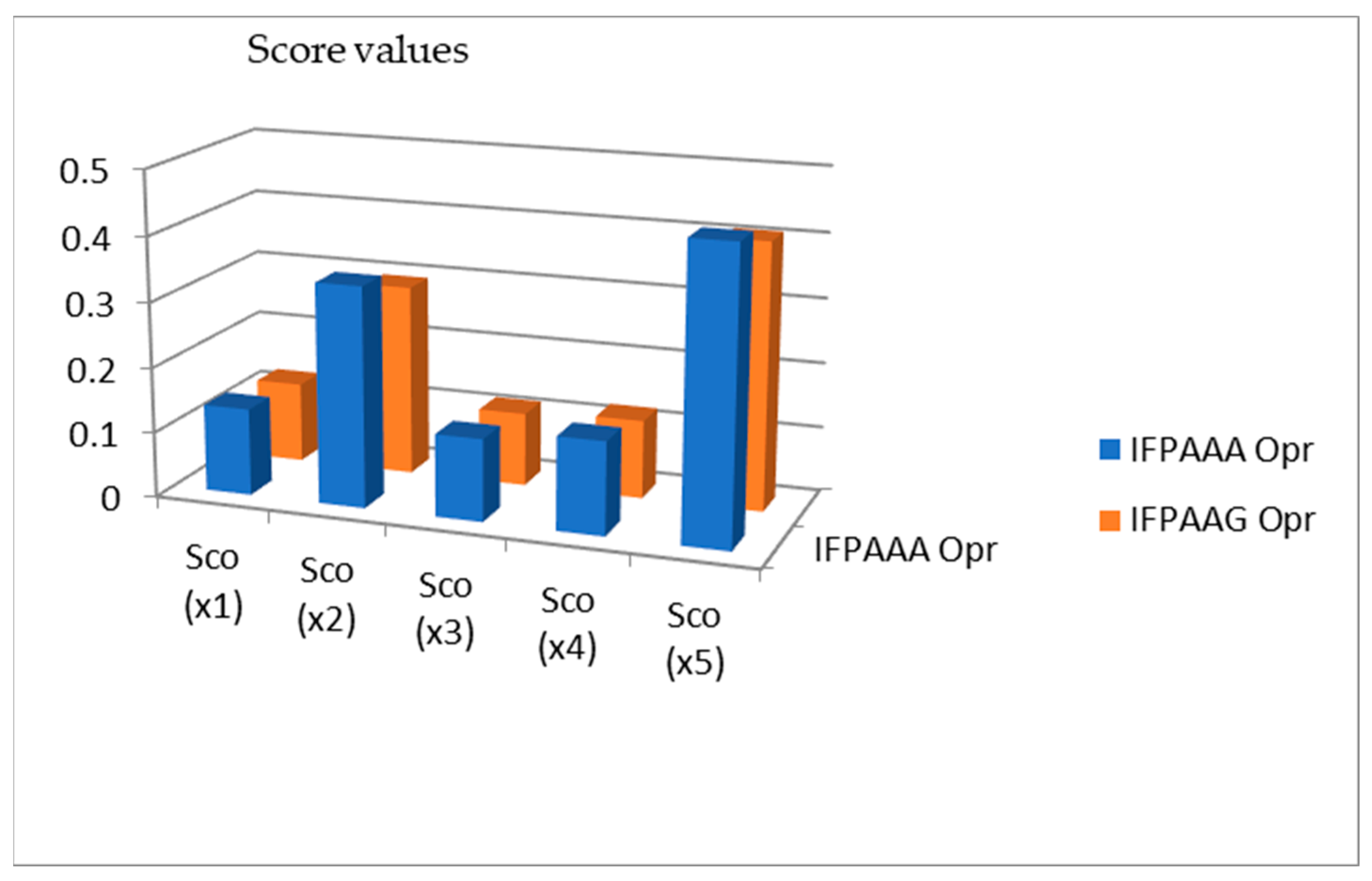
To propose prioritized AOs for IF information based on the Aczel–Alsina TN and TCN, i.e., IFPAAA and IFPAAG operators, to overcome shortcomings.
(2)
To study the importance of the proposed IFPAAA and IFPAAG operators.
(3)
To study some properties of the proposed prioritized AOs.
(4)
To apply the IFPAAA and IFPAAG operators in a MAGDM problem.
(5)
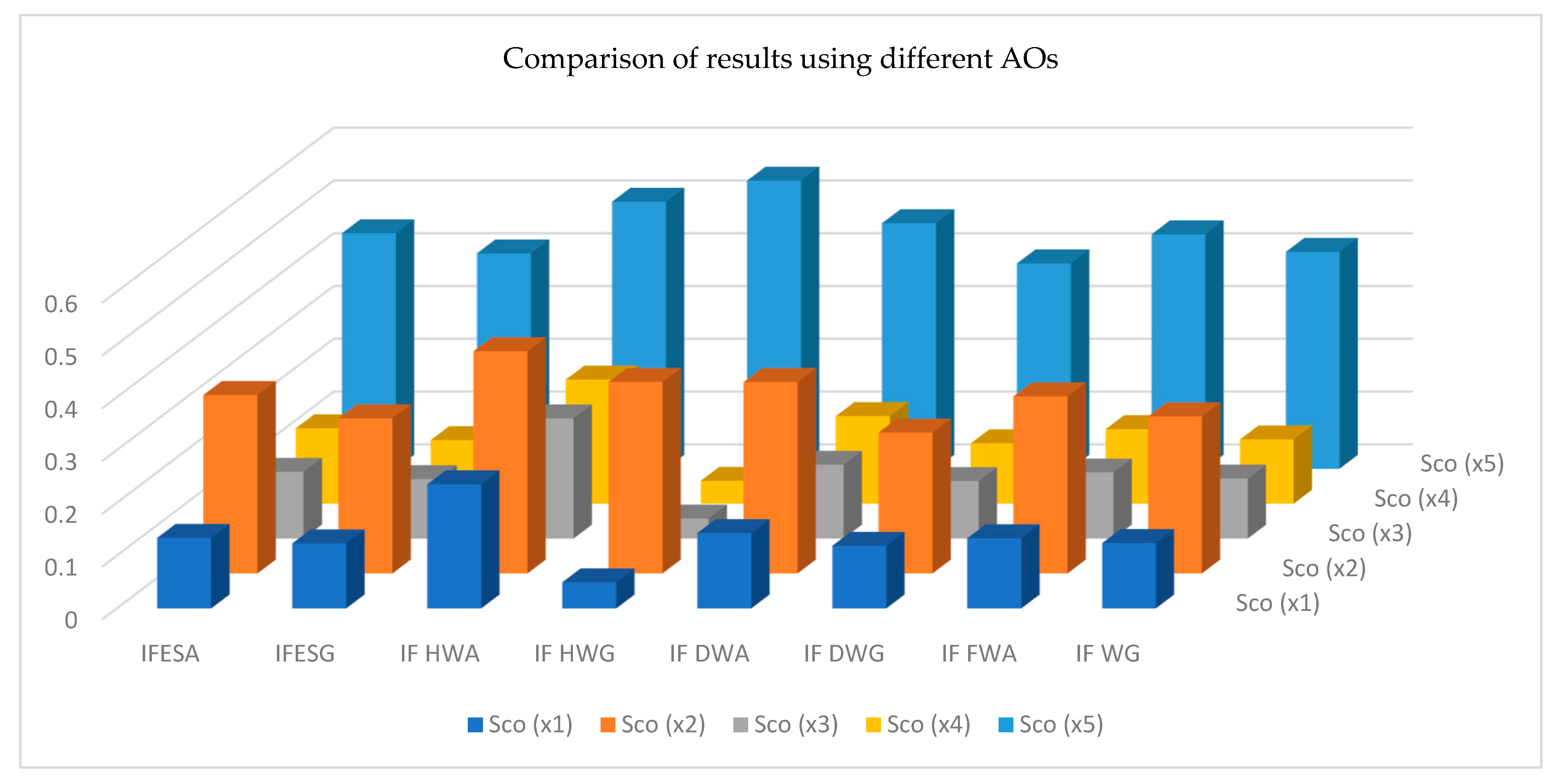
To compare the results obtained using the proposed prioritized AOs of IFVs with other existing AOs.
This paper is organized as follows: Section 1 covers the introduction and brief history of previous concepts with relevant literature. In Section 2, we discuss some basic concepts of IFSs, the Aczel–Alsina TN and TCN, and Aczel–Alsina AOs. In Section 3, we propose the IFPAAA and IFPAAG operators and study their relevant properties. In Section 4, we discuss the MAGDM algorithm based on IFPAAA and IFPAAG operators, followed by a comprehensive decision-making example in Section 5. In Section 6, we establish a comparison study of the proposed and existing theories, while in Section 7, we summarize the article with some concluding remarks.

2. Preliminaries

As an extension of an FS, Atanassov [2] proposed IFSs. IFSs deliver both an MD and an NMD simultaneously, whereas fuzzy sets only deliver the MD of an element in a specific set. The MD in the context of fuzzy sets is a real number between 0 and   1 . Similar results are obtained for the NMD, and additionally the sum of the two degrees is less than or equal to 1 . IFSs are defined by means of the following:
Definition 1
[2]. Let F be considered a universe of discourse; an IFS in F is an expression ϱ given by
β = { ( ξ , γ β ( ξ ) , δ β ( ξ ) : ξ F ) }
where   γ β : F [ 0 , 1 ] ,   δ β : F [ 0 , 1 ] , including the condition   0 γ β ( ξ ) + δ β ( ξ ) 1 , for each   ξ in   F . The numbers   γ β ( ξ )   and   δ β ( ξ ) serve as the MD and NMD of the element   ξ   in the set   F , respectively. For every IFS   β in   F , we denote   π β ( ξ ) = 1 γ β ( ξ ) δ β ( ξ ) ,   ξ F . Then   π β ( ξ ) is known as the hesitancy degree (HD) of   ξ   to   β . Especially, if   π β ( ξ ) = 1 γ β ( ξ ) δ β ( ξ ) = 0 ,     ξ F   , then the IFS   β is diminished to an FS. Furthermore,   ( γ β ( ξ ) , δ β ( ξ ) ) is known as the intuitionistic fuzzy value (IFV).
Definition 2
[12]. Let   β 1 = ( γ β 1 , δ β 1 )   be an IFV. Then
S c o ( β 1 ) = γ β 1 δ β 1
is the score value of   β 1 .
Definition 3
[12]. Let   β 1 = ( γ β 1 , δ β 1 )   be an IFV. Then
A c c   ( β 1 ) = γ β 1 + δ β   1
is the degree of accuracy of   β 1 .
(1)
If   S c o ( β 1 ) < S c o ( β 2 ) , then β 1 has less preference than   β 2 .
(2)
If   S c o ( β 1 ) = S c o ( β 2 ) , then β 1 and   β 2 are the same.
(3)
If   A c c   ( β 1 ) < A c c   ( β 2 ) , then β 1 has less preference than   β 2 .
(4)
If   A c c   ( β 1 ) = A c c   ( β 2 ) , then β 1 and   β 2 are the same.
Definition 4.
The Aczel–Alsina t-norm ( T A դ ) դ ϵ [ 0 , ] is ascertained by
( T A դ ) ( , v ) = { T D ( , v )             i f     դ = 0   m i n ( , v )       i f   դ = e ( ( l n ) դ + ( l n v ) դ ) 1 դ                 o t h e r w i s e
The Aczel–Alsina t-conorm ( S A դ ) դ ϵ [ 0 , ] is ascertained by
( S A դ ) ( , v ) = { S D ( , v )             i f     դ = 0   m a x ( , v )       i f   դ = 1 e ( ( l n ( 1 ) ) դ + ( l n ( 1 v ) ) դ ) 1 դ                 o t h e r w i s e
Limiting values: T A = m i n , T A 0 = T D ,   T A 1 = T p , S A = m a x , S A 0 = S D , and   S A 1 = S p . The t-norm T A դ and t-conorm   S A դ are dual with regard to each other for all դ ϵ [ 0 , ] . Both the Aczel–Alsina t-norm family and the Aczel–Alsina t-conorm family show strictly expanding and strictly reducing trends, respectively.
Furthermore, the Aczel–Alsina t-norms are the only ones that truly satisfy the equivalence   T ( λ , v λ ) = T ( , v ) λ for any λ > 0 and , v [ 0 , 1 ] .
Definition 5
[17]. Let   β = ( γ β , δ β ) ,   β 1 = ( γ β 1 , δ β 1 ) , and   β 2 = ( γ β 2 , δ β 2 ) be three IFVs, դ 1   and Φ 0 . Then the Aczel–Alsina t-norm and t-conorm operations of IFVs are defined as:
(i)
β 1 β 2 = ( 1 e ( ( l n ( 1 γ β 1 ) ) դ + ( l n ( 1 γ β 2 ) ) դ ) 1 / դ , e ( ( l n ( δ β 1 ) ) դ + ( l n ( δ β 2 ) ) դ ) 1 / դ ) ,
(ii)
β 1 β 2 = ( e ( ( l n ( γ β 1 ) ) դ + ( l n ( γ β 2 ) ) դ ) 1 / դ , 1 e ( ( l n ( 1 δ β 1 ) ) դ + ( l n ( 1 δ β 2 ) ) դ ) 1 / դ ) ,
(iii)
Φ β = (   1 e ( Φ ( l n ( 1 γ β ) ) դ ) 1 / դ ,   e ( Φ ( l n ( δ β ) ) դ ) 1 / դ ) ,
(iv)
β Φ = ( e ( Φ ( l n ( γ β ) ) դ ) 1 / դ ,   1 e ( Φ ( l n ( 1 δ β ) ) դ ) 1 / դ ) ,
Definition 6.
Let   β j = ( γ β j , δ β J ) be a collection of IFVs and T 1 j = 1 ϑ T j β j = ( T 1 j = 1 ϑ T j β 1 , T 1 j = 1 ϑ T j β 2 , T 1 j = 1 ϑ T j β ϑ ) T shows a weight vector of β j ( j = 1 , 2 , , ϑ ) in a manner allowing β j [ 0 , 1 ] , j = 1 , 2 , ϑ and   j = 1 ϑ ϑ j = 1 .
So, the IFPAAA operator of dimension ϑ is a function IFPAAA:   L * ϑ L *  
I F P A A A ( β 1 , β 2 , , β ϑ ) = ( ( 1 j = 1 ϑ ( 1 γ β j L ) ϑ j , 1 j = 1 ϑ ( 1 γ β j U ) ϑ j ) , ( j = 1 ϑ ( δ β j L ) ϑ j , j = 1 ϑ ( δ β j U ) ϑ j ) )

3. Intuitionistic Fuzzy Prioritized Aczel–Alsina Averaging Aggregation Operators

In this section, we present a few IFPAAA operators by means of the Aczel–Alsina operations. Throughout this article, ( j = 1 , 2 , ϑ )   will stand for indexing terms.
Definition 7.
Let   β j = ( γ β j , δ β j ) be an accumulation of IFVs. Then, the (IFPAAA) operator is a function   I F P A A A : L * ϑ L * and defined as:
I F P A A A ( β 1 , β 2 , β ϑ ) = j = 1 ϑ T j j = 1 ϑ T j β j
Using Aczel–Alsina operations on IFVs, we prove the following theorem.
Theorem 1.
Let   β j = ( γ β j , δ β J ) be a collection of IFVs. Then, the aggregated value of   β j   utilizing the IFPAAA operator is also an IFV, given by:
I F P A A A ( β 1 , β 2 , β ϑ ) = ( 1 e ( j = 1 ϑ T j j = 1 ϑ T j ( l n ( 1 γ β j ) ) դ ) 1 դ , e ( j = 1 ϑ T j j = 1 ϑ T j ( l n ( δ β j ) ) դ ) 1 / դ )        
Proof. 
Theorem 1 can be demonstrated in the following way using the mathematical induction approach.
(I)
For ϑ = 2 , using Aczel–Alsina operations of IFVs, we obtain
T 1 j = 1 ϑ T j β 1 = ( 1 e ( T 1 j = 1 ϑ T j ( l n ( 1 γ β 1 ) ) դ ) 1 / դ , e ( T 1 j = 1 ϑ T j ( l n ( δ β 1 ) ) դ ) 1 / դ ) T 2 j = 1 ϑ T j β 2 = ( 1 e ( T 2 j = 1 ϑ T j ( l n ( 1 γ β 2 ) ) դ ) 1 դ , e ( T 2 j = 1 ϑ T j ( l n ( δ β 2 ) ) դ ) 1 դ )   I F P A A A ( β 1 , β 2 ) = T 1 j = 1 2 T j β 1 T 2 j = 1 2 T j β 2 = ( 1 e ( T 1 j = 1 2 T j ( l n ( 1 γ β 1 ) ) դ ) 1 դ , e ( T 1 j = 1 2 T j ( l n ( δ β 1 ) ) դ ) 1 դ ) ( 1 e ( T 2 j = 1 2 T j ( l n ( 1 γ β 2 ) ) դ ) 1 / դ , e ( T 2 j = 1 2 T j ( l n ( δ β 2 ) ) դ ) 1 / դ ) = ( 1 e ( T 1 j = 1 2 T j ( l n ( 1 γ β 1 ) ) դ + T 2 j = 1 2 T j ( l n ( 1 γ β 2 ) ) դ ) 1 դ , e ( T 1 j = 1 2 T j ( l n ( δ β 1 ) ) դ + T 2 j = 1 2 T j ( l n ( δ β 2 ) ) դ ) 1 / դ ) = ( 1 e ( j = 1 ϑ T j j = 1 2 T j ( l n ( 1 γ β j ) ) դ ) 1 / դ , e ( j = 1 ϑ T j j = 1 2 T j ( l n ( δ β j ) ) դ ) 1 / դ )
Hence, Equation (3) is true for   ϑ = 2 .
(II)
Assume that Equation (3) is true for ϑ = k , then we have
I F P A A A ( β 1 , β 2 , β k ) = j = 1 k T j j = 1 k T j ( β j ) = ( 1 e ( j = 1 k T j j = 1 k T j ( l n ( 1 γ β j ) ) դ ) 1 դ , e ( j = 1 k T j j = 1 k T j ( l n ( δ β j ) ) դ ) 1 / դ )
Now for   ϑ = k + 1 , we obtain
I F P A A A ( β 1 , β 2 , β k + 1 ) = j = 1 k T j j = 1 k + 1 T j ( β j ) T k + 1 j = 1 k + 1 T j ( β k + 1 )
= ( ( 1 e ( j = 1 k T j j = 1 k + 1 T j ( l n ( 1 γ β j ) ) դ ) 1 դ , e ( j = 1 k T j j = 1 k + 1 T j ( l n ( δ β j ) ) դ ) 1 դ ) ( 1 e ( T k + 1 j = 1 k + 1 T j ( l n ( 1 γ β k + 1 ) ) դ ) 1 / դ , e ( T k + 1 j = 1 k + 1 T j ( l n ( 1 δ β k + 1 ) ) դ ) 1 / դ ) )
= ( 1 e ( j = 1 k + 1 T j j = 1 k + 1 T j ( l n ( 1 γ β j ) ) դ ) 1 / դ , e ( j = 1 k + 1 T j j = 1 k + 1 T j ( l n ( δ β j ) ) դ ) 1 / դ )
Equation (3) is therefore valid for ϑ = k + 1 .
We conclude that Equation (3) holds for any value of ϑ as a result of forms (I) and (II).
Every aggregation operator must satisfy the boundedness and monotonicity condition; idempotency is also one the famous properties of aggregation. Below, we show that the IFPAAA operator satisfies the condition of boundedness, monotonicity, idempotency.
The following properties, given in Theorems 2, 3, and 4, are likely to satisfy using the IFPAAA operator. □
Theorem 2.
If all   β j = ( γ β j , δ β j ) = ( γ β , δ β ) = β , that is β j = β for all   j , then   I F P A A A ( β 1 , β 2 , , β ϑ ) = β .
Proof. 
Since   β j = ( γ β j , δ β j ) = β = ( γ β , δ β ) , then we have by Equation (3)
I F P A A A ( β 1 , β 2 , β ϑ ) = ( 1 e ( j = 1 ϑ T j j = 1 ϑ T j ( l n ( 1 γ β j ) ) դ ) 1 / դ , e ( j = 1 ϑ T j j = 1 ϑ T j ( l n ( δ β j ) ) դ ) 1 / դ ) = ( 1 e ( ( l n ( 1 γ β ) ) դ ) 1 / դ , e ( ( l n ( δ β ) ) դ ) 1 / դ ) = ( 1 e l n ( 1 γ β ) , e l n δ β ) = ( γ β , δ β ) = β
Thus, I F P A A A ( β 1 , β 2 , , β ϱ ) = β holds. □
Theorem 3.
Let   β j = ( γ β j , δ β j ) be a collection of IFVs. Let β = m i n ( β 1 , β 2 , , β ϑ ) and   β + = m a x ( β 1 , β 2 , , β ϑ ) . Then   β I F P A A A ( β 1 , β 2 , , β ϑ ) β + .
Proof. 
Let   β j = ( γ β j , δ β j )   be a collection of IFVs. Let β = m i n ( β 1 , β 2 , , β ϑ ) = ( γ β , δ β )   and   β + = m a x ( β 1 , β 2 , , β ϑ ) = ( γ β + , δ β + ) . Hence, there are the subsequent inequalities:
1 e ( j = 1 ϑ T j j = 1 ϑ T j ( l n ( 1 γ β ) ) դ ) 1 դ 1 e ( j = 1 ϑ T j j = 1 ϑ T j ( l n ( 1 γ β j ) ) դ ) 1 դ 1 e ( j = 1 T j j = 1 ϑ T j ( l n ( 1 γ β j ) ) դ ) 1 / դ e ( j = 1 ϑ T j j = 1 ϑ T j ( l n ( δ β + ) ) դ ) 1 / դ e ( j = 1 ϑ T j j = 1 ϑ T j ( l n ( δ β j ) ) դ ) 1 / դ e ( j = 1 ϑ T j j = 1 ϑ T j ( l n ( δ β ) ) դ ) 1 / դ
Therefore, β I F P A A A ( β 1 , β 2 , , β ϑ β + ) . □
Theorem 4.
Let   β j   and   β j be two sets of IFVs. If β j   β j for all   j , then
I F P A A A ( β 1 , β 2 , , β ϑ ) I F P A A A ( β 1 , β 2 , , β ϑ )
Proof. 
Straightforward. □
Theorem 5.
Let   β j = ( γ β j , δ β j ) be a collection of IFVs, where   T j = k = 1 j 1 S   ( β k ) ( j = 2 , ϑ ) , T 1 = 1   , and   S   ( β k ) is the score of IFVs ( β k ) .   If α = ( γ α , δ α ) is IFVs on   k , then:
I F P A A A ( β 1 α , β 2 α , , β ϑ α ) = I F P A A A ( β 1 , β 2 , , β ϑ ) α
Proof. 
First, we compute I F P A A A ( β 1 α , β 2 α , , β ϑ α ) .
I F P A A A ( β 1 , β 2 , β ϑ ) = ( 1 e ( j = 1 ϑ T j j = 1 ϑ T j ( l n ( 1 γ β j ) ) դ ) 1 / դ , e ( j = 1 ϑ T j j = 1 ϑ T j ( l n ( δ β j ) ) դ ) 1 / դ ) β j α = ( 1 e ( ( l n ( 1 γ β j ) ) դ + ( l n ( 1 γ α ) ) դ ) 1 / դ , e ( ( l n ( δ β j ) ) դ + ( l n ( δ α ) ) դ ) 1 / դ ) I F P A A A ( β 1 α , β 2 α , , β ϑ α ) = ( 1 e ( j = 1 ϑ T j j = 1 ϑ T j ( l n ( 1 ( 1 e ( ( l n ( 1 γ β j ) ) դ + ( l n ( 1 γ α ) ) դ ) 1 դ ) ) ) դ ) 1 դ , e ( j = 1 ϑ T j j = 1 ϑ T j ( l n ( e ( ( l n ( δ β j ) ) դ + ( l n ( δ α ) ) դ ) 1 / դ ) ) դ ) 1 / դ ) I F P A A A ( β 1 α , β 2 α , , β ϑ α ) = ( 1 e ( ( j = 1 ϑ T j j = 1 ϑ T j ( l n ( 1 γ β j ) ) դ ) + ( l n ( 1 ( γ α ) ) ) դ ) 1 դ , e ( ( j = 1 ϑ T j j = 1 ϑ T j ( l n ( δ β j ) ) դ ) + ( l n ( δ α ) ) դ ) 1 / դ ) I F P A A A ( β 1 α , β 2 α , , β ϑ α )   = ( 1 e ( j = 1 ϑ T j j = 1 ϑ T j ( l n ( 1 γ β j α ) ) դ ) 1 / դ , e ( j = 1 ϑ T j j = 1 ϑ T j ( l n ( δ β j α ) ) դ ) 1 / դ )
Then, we make an expression for I F P A A A ( β 1 , β 2 , , β ϑ ) α
I F P A A A ( β 1 , β 2 , β ϑ ) = ( 1 e ( j = 1 ϑ T j j = 1 ϑ T j ( l n ( 1 γ β j ) ) դ ) 1 / դ , e ( j = 1 ϑ T j j = 1 ϑ T j ( l n ( δ β j ) ) դ ) 1 / դ ) I F P A A A ( β 1 , β 2 , β ϑ ) α = ( 1 e ( j = 1 ϑ T j j = 1 ϑ T j ( l n ( 1 γ β j ) ) դ ) 1 դ , e ( j = 1 ϑ T j j = 1 ϑ T j ( l n ( δ β j ) ) դ ) 1 / դ ) α I F P A A A ( β 1 , β 2 , β ϑ ) α = ( 1 e ( j = 1 ϑ T j j = 1 ϑ T j ( l n ( 1 γ β j ) ) դ ) 1 դ , e ( j = 1 ϑ T j j = 1 ϑ T j ( l n ( δ β j ) ) դ ) 1 / դ ) ( γ α , δ α ) I F P A A A ( β 1 , β 2 , β ϑ ) α = ( 1 e ( ( l n ( 1 ( 1 e ( j = 1 ϑ T j j = 1 ϑ T j ( l n ( 1 γ β j ) ) դ ) 1 դ ) ) ) դ + ( l n ( 1 ( γ α ) ) ) դ ) 1 դ , e ( ( l n ( e ( j = 1 ϑ T j j = 1 ϑ T j ( l n ( δ β j ) ) դ ) 1 / դ ) ) դ + ( l n ( δ α ) ) դ ) 1 / դ ) = ( 1 e ( ( j = 1 ϑ T j j = 1 ϑ T j ( l n ( 1 γ β j ) ) դ ) + ( l n ( 1 ( γ α ) ) ) դ ) 1 դ , e ( ( j = 1 ϑ T j j = 1 ϑ T j ( l n ( δ β j ) ) դ ) + ( l n ( δ α ) ) դ ) 1 / դ )
Hence:
I F P A A A ( β 1 α , β 2 α , , β ϑ α ) = I F P A A A ( β 1 , β 2 , , β ϑ ) α
Theorem 6.
Let   β j = ( γ β j , δ β j ) be a collection of IFVs, and T j = k = 1 j 1 S   ( β k ) ( j = 2 , ϑ ) , T 1 = 1   , and   S   ( β k ) is the score of β k , if Φ > 0 , then:
I F P A A A ( Φ β 1 , Φ β 2 , , Φ β ϑ ) = Φ I F P A A A ( β 1 , β 2 , , β ϑ )
Proof. 
We have the following based on the operational laws listed in Section 2:
Φ β = (     1 e ( Φ ( l n ( 1 γ β j ) ) դ ) 1 / դ ,   e ( Φ ( l n ( δ β j ) ) դ ) 1 / դ )
According to Theorem 1, we have:
IFPAAA ( Φ β 1 , Φ β 2 , , Φ β ϑ ) = ( 1 e ( j = 1 ϑ T j j = 1 ϑ T j ( ln ( 1 ( 1 e ( Φ ( ln ( 1 γ β j ) ) դ ) 1 դ ) ) ) դ ) 1 դ , e ( j = 1 ϑ T j j = 1 ϑ T j ( ln ( e ( Φ ( ln ( δ β j ) ) դ ) 1 / դ ) ) դ ) 1 / դ ) = ( 1 e ( j = 1 ϑ T j j = 1 ϑ T j ( ( Φ ( ln ( 1 γ β j ) ) դ ) ) ) 1 դ , e ( j = 1 ϑ T j j = 1 ϑ T j ( ( Φ ( ln ( δ β j ) ) դ ) ) ) 1 դ )   Φ I F P A A A ( β 1 , β 2 , , β ϑ ) = Φ ( 1 e ( j = 1 ϑ T j j = 1 ϑ T j ( l n ( 1 γ β j ) ) դ ) 1 դ , e ( j = 1 ϑ T j j = 1 ϑ T j ( l n ( δ β j ) ) դ ) 1 դ ) = (     1 e ( Φ ( l n ( 1 ( 1 e ( j = 1 ϑ T j j = 1 ϑ T j ( l n ( 1 γ β j ) ) դ ) 1 դ ) ) ) դ ) 1 դ ,   e ( Φ ( l n ( e ( j = 1 ϑ T j j = 1 ϑ T j ( l n ( δ β j ) ) դ ) 1 / դ ) ) դ ) 1 / դ ) = ( 1 e ( Φ ( ( j = 1 ϑ T j j = 1 ϑ T j ( ln ( 1 γ β j ) ) դ ) ) ) 1 / դ , e ( Φ ( ( j = 1 ϑ T j j = 1 ϑ T j ( ln ( δ β j ) ) դ ) ) ) 1 / դ )
Hence:
I F P A A A ( Φ β 1 , Φ β 2 , , Φ β ϑ ) = Φ I F P A A A ( β 1 , β 2 , , β ϑ )
Theorem 7.
Let   β j = ( γ β j , δ β j ) be a collection of IFVs, and   T j = k = 1 j 1 S   ( β k ) ( j = 2 , ϑ ) , T 1 = 1 , and   S   ( β k ) is the score of IFVs   β k , if   Φ > 0 , α = ( γ α , δ α )   is a IFVs on   k . Then
I F P A A A ( Φ β 1 α , Φ β 2 α , , Φ β ϑ α ) = Φ I F P A A A ( β 1 , β 2 , , β ϑ ) α
Proof. 
  I F P A A A ( Φ β 1 α , Φ β 2 α , , Φ β ϑ α ) = Φ I F P A A A ( β 1 , β 2 , , β ϑ ) α I F P A A A ( β 1 , β 2 , β ϑ ) = ( 1 e ( j = 1 ϑ T j j = 1 ϑ T j ( l n ( 1 γ β j ) ) դ ) 1 / դ , e ( j = 1 ϑ T j j = 1 ϑ T j ( l n ( δ β j ) ) դ ) 1 / դ ) Φ I F P A A A ( β 1 , β 2 , , β ϑ ) = Φ ( 1 e ( j = 1 ϑ T j j = 1 ϑ T j ( l n ( 1 γ β j ) ) դ ) 1 / դ , e ( j = 1 ϑ T j j = 1 ϑ T j ( l n ( δ β j ) ) դ ) 1 / դ ) Φ I F P A A A ( β 1 , β 2 , , β ϑ ) = (     1 e ( Φ ( j = 1 ϑ T j j = 1 ϑ T j ( l n ( 1 γ β j ) ) դ ) ) 1 / դ ,   e ( Φ ( j = 1 ϑ T j j = 1 ϑ T j ( l n ( δ β j ) ) դ ) ) 1 / դ ) Φ I F P A A A ( β 1 , β 2 , , β ϑ ) α = (     1 e ( Φ ( j = 1 ϑ T j j = 1 ϑ T j ( l n ( 1 γ β j ) ) դ ) ) 1 դ ,   e ( Φ ( j = 1 ϑ T j j = 1 ϑ T j ( l n ( δ β j ) ) դ ) ) 1 դ ) ( γ α , δ α ) Φ I F P A A A ( β 1 , β 2 , , β ϑ ) α = ( 1 e ( ( Φ ( j = 1 ϑ T j j = 1 ϑ T j ( l n ( 1 γ β j ) ) դ ) ) + ( l n ( 1 γ α ) ) դ ) 1 դ , e ( ( ( Φ ( j = 1 ϑ T j j = 1 ϑ T j ( l n ( δ β j ) ) դ ) ) ) + ( l n ( δ α ) ) դ ) 1 / դ ) I F P A A A ( Φ β 1 α , Φ β 2 α , , Φ β ϑ α ) Φ β j = (     1 e ( Φ ( l n ( 1 γ β j ) ) դ ) 1 / դ ,   e ( Φ ( l n ( δ β j ) ) դ ) 1 / դ ) Φ β j α = (     1 e ( Φ ( l n ( 1 γ β j ) ) դ ) 1 / դ ,   e ( Φ ( l n ( δ β j ) ) դ ) 1 / դ ) ( γ α , δ α ) Φ β j α = ( 1 e ( ( l n ( 1 ( 1 e ( Φ ( l n ( 1 γ β j ) ) դ ) 1 դ ) ) ) դ + ( l n ( 1 γ α ) ) դ ) 1 դ , e ( ( l n ( e ( Φ ( l n ( δ β j ) ) դ ) 1 / դ ) ) դ + ( l n ( δ α ) ) դ ) 1 / դ ) = ( 1 e ( j = 1 ϑ T j j = 1 ϑ T j ( l n ( 1 ( 1 e ( ( l n ( 1 ( 1 e ( Φ ( l n ( 1 γ β j ) ) դ ) 1 դ ) ) ) դ + ( l n ( 1 γ α ) ) դ ) 1 դ ) ) ) դ ) 1 դ , e ( j = 1 ϑ T j j = 1 ϑ T j ( l n ( e ( ( l n ( e ( Φ ( l n ( δ β j ) ) դ ) 1 / դ ) ) դ + ( l n ( δ α ) ) դ )       1 / դ ) ) դ ) 1 / դ ) ( 1 e ( j = 1 ϑ T j j = 1 ϑ T j ( Φ ( ( l n ( 1 γ β j ) ) դ ) ) + ( l n ( 1 γ α ) ) դ ) 1 դ , e ( j = 1 ϑ T j j = 1 ϑ T j ( ( Φ ( ( l n ( δ β j ) ) դ ) ) ) + ( l n ( δ α ) ) դ ) 1 / դ )
Theorem 8.
Let β j = ( γ β j , δ β j )   and   α j = ( γ α j , δ α j ) be two collections of IFVs, and   T j = k = 1 j 1 S   ( β k ) ( j = 2 , ϑ ) , T 1 = 1 , and S   ( β k )   is the score of IFVs   β k . Then
I F P A A A ( β 1 α 1 , β 2 α 2 , , β ϑ α ϑ ) = I F P A A A ( β 1 , β 2 , , β ϑ )   I F P A A A ( α 1 , α 2 , , α ϑ )
Proof. 
According to Theorem 1, we have:
β j α j = ( 1 e ( ( l n ( 1 γ β j ) ) դ + ( l n ( 1 γ α j ) ) դ ) 1 / դ , e ( ( l n ( δ β j ) ) դ + ( l n ( δ α j ) ) դ ) 1 / դ ) I F P A A A ( β 1 , β 2 , , β ϑ )   = ( 1 e ( j = 1 ϑ T j j = 1 ϑ T j ( l n ( 1 γ β j ) ) դ ) 1 / դ , e ( j = 1 ϑ T j j = 1 ϑ T j ( l n ( δ β j ) ) դ ) 1 / դ ) I F P A A A ( β 1 α 1 , β 2 α 2 , , β ϑ α ϑ ) = ( 1 e ( j = 1 ϑ T j j = 1 ϑ T j ( ( ( l n ( 1 γ β j ) ) դ + ( l n ( 1 γ α j ) ) դ ) ) ) 1 դ , e ( j = 1 ϑ T j j = 1 ϑ T j ( ( ( l n ( δ β j ) ) դ + ( l n ( δ α j ) ) դ ) ) ) 1 / դ ) I F P A A A ( β 1 , β 2 , , β ϑ )   I F P A A A ( α 1 , α 2 , , α ϑ ) = ( ( 1 e ( j = 1 ϑ T j j = 1 ϑ T j ( l n ( 1 γ β j ) ) դ ) 1 դ , e ( j = 1 ϑ T j j = 1 ϑ T j ( l n ( δ β j ) ) դ ) 1 դ ) ( 1 e ( j = 1 ϑ T j j = 1 ϑ T j ( l n ( 1 γ α j ) ) դ ) 1 / դ , e ( j = 1 ϑ T j j = 1 ϑ T j ( l n ( δ α j ) ) դ ) 1 / դ ) ) = ( 1 e ( ( l n ( 1 ( 1 e ( j = 1 ϑ T j j = 1 ϑ T j ( l n ( 1 γ β j ) ) դ ) 1 դ ) ) ) դ + ( l n ( 1 ( 1 e ( j = 1 ϑ T j j = 1 ϑ T j ( l n ( 1 γ α j ) ) դ ) 1 դ ) ) ) դ ) 1 դ , e ( ( l n ( e ( j = 1 ϑ T j j = 1 ϑ T j ( l n ( δ β j ) ) դ ) 1 դ ) ) դ + ( l n ( e ( j = 1 ϑ T j j = 1 ϑ T j ( l n ( δ α j ) ) դ ) 1 / դ ) ) դ ) 1 / դ   ) = ( 1 e ( j = 1 ϑ T j j = 1 ϑ T j ( ( l n ( 1 γ β j ) ) դ + ( l n ( 1 γ α j ) ) դ ) ) 1 դ , e ( j = 1 ϑ T j j = 1 ϑ T j ( ( ( l n ( δ β j ) ) դ + ( l n ( δ α j ) ) դ ) ) ) 1 / դ )
Definition 8.
Let   β j = ( γ β j , δ β j ) be a collection of IFVs, and let   I F P A A G : L * ϑ L * if:
I F P A A G ( β 1 , β 2 , β ϑ ) = j = 1 ϑ β j T j j = 1 ϑ T j
Then the function IFPAAG is called an interval-valued IFPAAG operator, where   T j = k = 1 j 1 S   ( β k ) ( j = 2 , ϑ ) , T 1 = 1   , and   S   ( β k ) is the score of IFVs   β k .
Theorem 9.
Let   β j = ( γ β j , δ β J )   be a collection of IFVs. Then, the aggregated value using the IFPAAG operator is also an IFV, given by:
I F P A A G ( β 1 , β 2 , β ϑ ) = ( , e ( j = 1 ϑ T j j = 1 ϑ T j ( l n ( δ β j ) ) դ ) 1 դ , 1 e ( j = 1 ϑ T j j = 1 ϑ T j ( l n ( 1 γ β j ) ) դ ) 1 / դ )
Proof. 
Theorem 9 can be demonstrated in the following way using the mathematical induction approach:
(I)
For ϑ = 2 , using Aczel–Alsina operations of IFVs, we obtain
β 1 T 1 j = 1 ϑ T j = ( e ( T 1 j = 1 ϑ T j ( l n ( δ β 1 ) ) դ ) 1 դ , 1 e ( T 1 j = 1 ϑ T j ( l n ( 1 γ β 1 ) ) դ ) 1 դ )   β 2 T 2 j = 1 ϑ T j = ( e ( T 2 j = 1 ϑ T j ( l n ( δ β 2 ) ) դ ) 1 / դ , 1 e ( T 2 j = 1 ϑ T j ( l n ( 1 γ β 2 ) ) դ ) 1 / դ ) I F P A A G ( β 1 , β 2 ) = β 1 T 1 j = 1 ϑ T j β 2 T 2 j = 1 ϑ T j = ( e ( T 1 j = 1 2 T j ( l n ( δ β 1 ) ) դ ) 1 / դ , 1 e ( T 1 j = 1 2 T j ( l n ( 1 γ β 1 ) ) դ ) 1 / դ ) ( e ( T 2 j = 1 2 T j ( l n ( δ β 2 ) ) դ ) 1 / դ , 1 e ( T 2 j = 1 2 T j ( l n ( 1 γ β 2 ) ) դ ) 1 / դ ) = ( , e ( T 1 j = 1 2 T j ( l n ( δ β 1 ) ) դ + T 2 j = 1 2 T j ( l n ( δ β 2 ) ) դ ) 1 դ , 1 e ( T 1 j = 1 2 T j ( l n ( 1 γ β 1 ) ) դ + T 2 j = 1 2 T j ( l n ( 1 γ β 2 ) ) դ ) 1 / դ ) = ( , e ( j = 1 ϑ T j j = 1 2 T j ( l n ( δ β j ) ) դ ) 1 / դ , 1 e ( j = 1 ϑ T j j = 1 2 T j ( l n ( 1 γ β j ) ) դ ) 1 / դ , )
Hence, Equation (4) is true for   ϑ = 2 .
(II)
If Equation (4) holds true for ϑ = k , then we have
I F P A A G ( β 1 , β 2 , β k ) = j = 1 k β j T j j = 1 k T j = ( , e ( j = 1 k T j j = 1 k T j ( l n ( δ β j ) ) դ ) 1 դ , 1 e ( j = 1 k T j j = 1 k T j ( l n ( 1 γ β j ) ) դ ) 1 / դ )
Now, for   ϑ = k + 1 , we get
I F P A A G ( β 1 , β 2 , β k + 1 ) = j = 1 k β j T j j = 1 k + 1 T j β k + 1 T k + 1 j = 1 k + 1 T j ( e ( j = 1 k T j j = 1 k + 1 T j ( l n ( δ β j ) ) դ ) 1 դ , 1 e ( j = 1 k T j j = 1 k + 1 T j ( l n ( 1 γ β j ) ) դ ) 1 դ ) ( e ( T k + 1 j = 1 k + 1 T j ( l n ( 1 δ β k + 1 ) ) դ ) 1 / դ , 1 e ( T k + 1 j = 1 k + 1 T j ( l n ( 1 γ β k + 1 ) ) դ ) 1 / դ ) ( e ( j = 1 k + 1 T j j = 1 k + 1 T j ( l n ( δ β j ) ) դ ) 1 / դ , 1 e ( j = 1 k + 1 T j j = 1 k + 1 T j ( l n ( 1 γ β j ) ) դ ) 1 / դ )
Equation (4) is therefore valid for   ϑ = k + 1 .
We conclude that Equation (4) holds for any value of ϑ as a result of forms (I) and (II). The following properties, given in Theorems 10, 11, and 12, are likely to satisfy using the IFPAAG operator. □
Theorem 10.
If all   β j = ( γ β j , δ β j ) is a collection of IFVs where   T j = k = 1 j 1 S   ( β k ) ( j = 2 , ϑ ) , T 1 = 1   , and   S   ( β k ) is the score of IFVs ( β k ) , if all β j = β for all   j , then   I F P A A G ( β 1 , β 2 , , β ϑ ) =   β .
Proof. 
Since   β j = ( γ β j , δ β j ) = β = ( γ β , δ β ) , we then have, by Equation (4):
I F P A A G ( β 1 , β 2 , β ϑ ) = ( , e ( j = 1 ϑ T j j = 1 ϑ T j ( l n ( δ β j ) ) դ ) 1 / դ , 1 e ( j = 1 ϑ T j j = 1 ϑ T j ( l n ( 1 γ β j ) ) դ ) 1 / դ ) = ( , e ( ( l n ( δ β ) ) դ ) 1 / դ , 1 e ( ( l n ( 1 γ β ) ) դ ) 1 / դ ) = 1 e l n ( 1 γ β ) , e l n δ β = ( γ β , δ β ) = β
Thus, I F P A A G ( β 1 , β 2 , , β ϱ ) = β   holds. □
Theorem 11.
Let   β j = ( γ β j , δ β j ) be a collection of IFVs. Let β = m i n ( β 1 , β 2 , , β ϑ ) and   β + = m a x ( β 1 , β 2 , , β ϑ ) . Then   β I F P A A G ( β 1 , β 2 , , β ϑ ) β + .
Proof. 
Let   β j = ( γ β j , δ β j )   be a collection of IFVs. Let β = m i n ( β 1 , β 2 , , β ϑ ) = ( γ β , δ β )   and   β + = m a x ( β 1 , β 2 , , β ϑ ) = ( γ β + , δ β + ) . Hence, there are the subsequent inequalities:
1 e ( j = 1 ϑ T j j = 1 ϑ T j ( l n ( 1 γ β ) ) դ ) 1 դ 1 e ( j = 1 ϑ T j j = 1 ϑ T j ( l n ( 1 γ β j ) ) դ ) 1 դ 1 e ( j = 1 T j j = 1 ϑ T j ( l n ( 1 γ β j ) ) դ ) 1 / դ e ( j = 1 ϑ T j j = 1 ϑ T j ( l n ( δ β + ) ) դ ) 1 / դ e ( j = 1 ϑ T j j = 1 ϑ T j ( l n ( δ β j ) ) դ ) 1 / դ e ( j = 1 ϑ T j j = 1 ϑ T j ( l n ( δ β ) ) դ ) 1 / դ .  
Therefore, β I F P A A G ( β 1 , β 2 , , β ϑ β + ) . □
Theorem 12.
Let   β j = ( γ β j , δ β j ) be a collection of IFVs, where   T j = k = 1 j 1 S   ( β k ) ( j = 2 , ϑ ) , T 1 = 1   , and   S   ( β k ) is the score of IFVs ( β k ) . If α = ( γ α , δ α )   is IFVs on   k , then:
I F P A A G ( β 1 α , β 2 α , , β ϑ α ) = I F P A A G ( β 1 , β 2 , , β ϑ ) α
Proof. 
Theorem 5’s proof can be used to prove Theorem 12 as well. □
Theorem 13.
Let   β j = ( γ β j , δ β j ) be a collection of IFVs, where   T j = k = 1 j 1 S   ( β k ) ( j = 2 , ϑ ) , T 1 = 1   , and   S   ( β k ) is the score of IFVs ( β k ) . If r > 0 , then:
I F P A A G ( β 1 r , β 2 r , , β ϑ r ) = I F P A A G ( β 1 , β 2 , , β ϑ ) r
Proof. 
Theorem 6’s proof can be used to prove Theorem 13 as well. □
Theorem 14.
Let   β j = ( γ β j , δ β j ) be a collection of IFVs, where   T j = k = 1 j 1 S   ( β k ) ( j = 2 , ϑ ) , T 1 = 1   , and   S   ( β k ) is the score of IFVs ( β k ) . If   r > 0 , α = ( γ α , δ α ) is IFV on   k , then:
I F P A A G ( β 1 r α , β 2 r դ α , β ϑ r դ α ) = I F P A A G ( β 1 , β 2 , , β ϑ ) r դ α
Proof. 
Theorem 7’s proof can be used to prove Theorem 14 as well. □
Theorem 15.
Let β j = ( γ β j , δ β j ) and   α j = ( γ α j , δ α j ) be two collections of IFVs, and   T j = k = 1 j 1 S   ( β k ) ( j = 2 , ϑ ) , T 1 = 1 , and S   ( β k )   be the score of IFVs β k . Then
I F P A A G ( β 1 α 1 , β 2 α 2 , , β ϑ α ϑ ) = I F P A A G ( β 1 , β 2 , , β ϑ )   I F P A A G ( α 1 , α 2 , , α ϑ )
Proof. 
Theorem 8’s proof can be used to prove Theorem 15 as well. □

4. MAGDM Methods Using Investigated Operators Based on IFVs

In this section, we will create an MADM methodology based on the proposed aggregation operators under IFVs to illustrate reliability and effectiveness. It is assumed that the set of alternatives in a group decision-making problem is k = {k1, k2, … km}, and that the set of parameters in the problem is A = { a 1 , a 2 , , a n } and the parameters represented by the linear ordering are prioritized. a 1 > a 2 > a 3 , , a n shows that the a j criterion is more important than a j if j < i. E = { e 1 , e 2 , , e p } is the set of decision makers; there is a prioritization among the decision makers indicated by linear ordering. e 1 > e 2 > , , > e p shows that the e criterion is more important than e τ if < τ. Let   K q = ( K i j q ) m × n be an IFV-based decision matrix and K i j q = ( γ i j q , δ i j q ) denote the attribute value provided by the decision maker eq, which is expressed as IFVs, where ( γ i j q , δ i j q ) indicates the degree range that the alternative ki satisfies. The attribute c j expresses the decision maker   e q , such that ( γ i j q , δ i j q ) ( 0 , 1 ) , ( γ i j q + δ i j q ) 1 , i = 1 , 2 , m , j = 1 , 2 , n .
If all the attributes a j ( j = 1 , 2 , , n ) are of the same type, then the attribute values do not need normalization. Otherwise, we normalize the decision-maker matrix K q = ( K i j q ) m × n into R q = ( r i j q ) m × n , where:
r i j q = { k i j q ,   f o r   b e n e f i t   a t t r i b u t e   a j k i j q ,   f o r cos t   a t t r i b u t e   a j
Then, we utilize the IFPAAA operator to develop an approach to multi-criteria decision-making under an interval-valued IF environment; the main steps are as follows:
Step 1: on the basis of the following equations, calculate the values of T i j q , ( q = 1 , 2 , p ) :
    T j = k = 1 j 1 S   ( r i j q ) ( q = 2 , p ) ,   T i j 1 = 1
Step 2: Utilize the IFPAAA operator given by:
r i j = I F P A A A ( β i j 1 , β i j 2 , , β i j p ϑ ) = ( 1 e ( j = 1 ϑ T j j = 1 ϑ T j ( p ) ( l n ( 1 γ β j ) ) դ ) 1 / դ , e ( j = 1 ϑ T j j = 1 ϑ T j ( p ) ( l n ( δ β j ) ) դ ) 1 / դ )
or the IFPAAG operator:
r i j = I F P A A G ( β i j 1 , β i j 2 , β i j p ϑ ) = ( , e ( j = 1 ϑ T j j = 1 ϑ T j ( p ) ( l n ( δ β j ) ) դ ) 1 / դ , 1 e ( j = 1 ϑ T j j = 1 ϑ T j ( p ) ( l n ( 1 γ β j ) ) դ ) 1 / դ )
to aggregate all the individual IF decision matrixes R q = ( r i j q ) m × n ( q = 2 , p ) into the collective IF decision matrix R = ( r i j ) m × n .
Step 3: Calculate the values of T i j , ( i = 1 , 2 , m ,   j = 1 , 2 , n ) based on the following equations:
    T j = k = 1 j 1 S   ( r i j q ) ( q = 2 , p ) ,   T i j 1 = 1
Step 4: Aggregate the IFVs   r i j :
I F P A A A ( β 1 , β 2 , β ϑ ) = ( 1 e ( j = 1 ϑ T j j = 1 ϑ T j ( l n ( 1 γ β j ) ) դ ) 1 / դ , e ( j = 1 ϑ T j j = 1 ϑ T j ( l n ( δ β j ) ) դ ) 1 / դ )
or
I F P A A G ( β 1 , β 2 , β ϑ ) = ( , e ( j = 1 ϑ T j j = 1 ϑ T j ( l n ( δ β j ) ) դ ) 1 դ , 1 e ( j = 1 ϑ T j j = 1 ϑ T j ( l n ( 1 γ β j ) ) դ ) 1 դ )
Step 5: Rank all the alternatives by the score function described in Section 2:
S c o ( β i ) = γ β i δ β i     i = 1 , 2 , m
then, the bigger the value of S ( r i )   , the larger the overall IFVs   ( r i ) , and thus the alternative k i ( i = 1 , 2 , m ) .

5. Practical Example

In this example, we take the selection of a doctor for a hospital. Suppose a hospital needs a doctor (medical specialist). There is a committee whose job is to select the most suitable candidate among a finite list of doctors. The committee consists of the president as   e 1 , the psychologist as e 2 , and the medical specialist or dean as e 3 . These experts are responsible for the whole induction process. They made a strict evaluation of five candidates K i ( i = 1 , 2 , , 5 ) from four aspects, namely morality   a 1 , good communication skills a 2 , competence   a 3 , and compassion   a 4 . The hospital president has absolute priority in decision-making, and the medical expert and psychologist come next. In addition, this introduction will be in strict accordance with the president combining ability with political integrity. Then, the prioritization relationship for the criteria is as below, a 1 > a 2 > a 3 , , a n . Three decision makers evaluate the candidates K i ( i = 1 , 2 , 5 ) with respect to the attributes A j ( j = 1 , 2 , 4 ) and construct the following three IF decision matrixes:   D q = ( d i j q ) 5 × 4 ( q = 1 , 2 , 3 ) . Since all the attributes   A j ( j = 1 , 2 , , 5 ) are of a beneficial type, we do not need normalization. The experts evaluated the candidates K i ( i = 1 , 2 , 5 ) with respect to the attributes A j ( j = 1 , 2 , 4 ) and constructed the following three IF decision matrixes   D q = ( d i j q ) 5 × 4 ( q = 1 , 2 , 3 ) with all the attributes   A j ( j = 1 , 2 , , 5 ) given in Table 1, Table 2 and Table 3.
Since the attribute values do not need to be normalized after modifying the type, the major stages are as follows when using the IFPAAA operator:
Step 1: Calculate the values of T i j 1 , T i j 2 , T i j 3 based on
T i j 1 = ( 1 1 1 1 1 1 1 1 1 1 1 1 1 1 1         1 1 1 1 1 ) T i j 2 = ( 0.1 0.4 0.1 0.1 0.5 0.2 0.3 0.1 0.1 0.5 0.2 0.1 0.38 0.1 0.4         0.4 0.6 0.38 0.2 0.2 )   T i j 3 = ( 0.03 0.12 0.02 0.03 0.25 0.002 0.057 0.05 0.03 0.05 0.04 0.009 0.0988 0.018 0.192         0.124 0.006 0.038 0.004 0.004 )  
Step 2: Aggregate each individual IF decision matrix into the collective IF decision matrix R = ( r i j ) 5 × 4   using the IFPAAA operator R q = ( r i j q ) 4 × 5 ( q = 1 , 2 , 3 ) (Table 4).
Step 3: Calculate the values of T i j , ( i = 1 , 2 , m ,   j = 1 , 2 , n ) based on
T i j = ( 1 1 1 1 1 0.123 0.3572 0.1147 0.142 0.4766 0.022015 0.109698 0.018376 0.018168 0.183985 0.004804 0.011747 0.006208 0.002084 0.075814 )
Step 4: The IFPAAA operator can be used to combine all of the desired values r i j ( i = 1 , 2 , 5 ) on the ith line of R to obtain the overall preference values   r i . This information are given in Table 5.
Step 5: Determine each score for   r i ( 1 , 2 , 5 ) etc. as given in Table 6.
Since
S 5 > S 2 > S 4 > S 1 > S 3
we have
k 5 > k 2 > k 4 > k 1 > k 3
Therefore,   k 5 is the perfect selection.
The major steps are as follows based on the IFPAAG operator:
Step 1: Already performed.
Step 2: The individual IF decision matrix can be aggregated using the IVFPAAG operator R q = ( r i j q ) 4 × 5 ( q = 1 , 2 , 3 ) into the collective IF decision matrix R q = ( r i j q ) 4 × 5 (see Table 7).
Step 3: Calculate the values of T i j , ( i = 1 , 2 , m ,   j = 1 , 2 , n ) based on
T i j = ( 1 1 1 1 1 0.1187 0.3454 0.1095 0.1248 0.4695 0.017847 0.084959 0.014191 0.013564 0.159555 0.003386 0.008392 0.004623 0.001358 0.064536 )
Step 4: The IFPAAA operator can be used to combine all of the desired values r i j ( i = 1 ,   2 , 5 ) on the ith line of R to obtain the overall preference values   r i (see Table 8).
Step 5: Determine each score for   r i ( 1 , 2 , 5 ) etc. (see Table 9).
The data given in Table 9 can be geometrically seen in Figure 1 below.
Therefore, k 5 is the optimal choice. The ranking of the alternatives is the same for the IFPAAA and IFPAAG operators. The proposed operators are simplified to the standard IF aggregation procedures if the criteria and the decision-makers have the same priority level. However, these four criteria and the three decision-makers have different degrees of significance. For instance, it is quite difficult to choose the candidate if the hospital president gave him a low assessment. From a different angle, a candidate cannot be chosen if they have poor moral character, despite how well they have performed in other areas such as integrity, communication skills, professionalism, and emotional stability. As a result, we need to think about how the criteria, or the decision makers are ranked in importance; the IFPAAG and IFPAAA operators are helpful tools for handling such circumstances. According to the analysis above, our operators have several advantages over conventional IF operators, including the ability to deal with the IF environment and the consideration of optimization between the criteria and the decision makers, which makes it more feasible and useful.

6. Comparative Study

This section compares the aggregated results obtained using the IFPAAA and IFPAAG operators with a variety of other AOs of IFVs. These AOs include the IFWA operator [9], IFDWA operator [44], IFFWA operator [13], and IFHWA operator [14]. We solved the problem studied earlier using these suggested AOs and display the results in Table 10 below.
The IFPAAA and IFPAAG operators show that k 5 is the optimal option. Moreover, when we applied the AOs proposed by Xu [9], Xu and Yager [10], Huang [13], Zhang [14], and Seikh and Mandal [44], we obtained somewhat similar results. k 5 was proven to be the best alternative among them all. We claim that the results established by our proposed operators are better because our method considers the prioritization of attributes. Furthermore, in reference to Farahbod and Eftekhari [41], Aczel–Alsina t-norm-based aggregation is more reliable than other AOs. We can see that in the Dombi AOs proposed by Seikh and Mandal [44], where there is a slight change in the ranking results. The results obtained using Frank AOs by Zhang [14] also show a fluctuation in ranking order. However, the proposed results using the IFPAAA and IFPAAG operators give us a smooth ranking. A geometrical view of the comparative study is given in Figure 2.

7. Conclusions

In this paper, we analyzed the Aczel–Alsina AOs of IFVs. We embedded the concept of prioritization in the Aczel–Alsina AOs of IFVs and proposed the IFPAAA and IFPAAG operators. The significance of the proposed prioritized AOs based on the Aczel–Alsina t-norm and t-conorm lies in the fact that in real-life decision-making problems, the attributes sometimes need prioritization, and in some cases the decision makers have a priority level. For this purpose, we proposed the IFPAAA and IFPAAG operators and studied their properties. We established several other results as well. To see the impact of the proposed IFPAAA and IFPAAG operators, we presented a numerical example where the selection of a doctor for a hospital was carried out using an MAGDM algorithm. The proposed MAGDM method considered the prioritization relationship among criteria and decision makers, which allowed our technique to have wide pragmatic application possibilities. Furthermore, we compared our results with other AOs with the concept of prioritization, and the results were analyzed. We found that the results were similar and compatible. The advantages of the proposed work include the inclusion of prioritization in aggregation for uncertain information where two aspects of human opinion are involved. On the other hand, the existing AOs do not improve the flexibility of data aggregation. Thus, our suggested AOs are more competent and accurate when making decisions using IF information. The proposed work has its limitations when the information expressing uncertainty has more characteristics and can be extended to the environment of interval-valued IFSs [45]. We also aim to extend this work to the frame of complex IFSs [46], complex Pythagorean fuzzy sets [47], complex q-rung orthopedic fuzzy sets [48], and T-spherical fuzzy sets (TSFSs) [49]. The proposed Aczel–Alsina AOs can also be associated with Maclaurin symmetric mean operators [24] and Bonferroni mean operators [50].

Author Contributions

Conceptualization, M.S., K.U. and M.A.; methodology, M.S., K.U., D.P. and D.B.; software, M.S., M.A., D.P. and D.B.; validation, K.U., M.A., D.P. and D.B.; formal analysis, D.P., and D.B.; investigation, M.S., K.U., M.A.; resources, K.U., D.P., and D.B.; writing—original draft preparation, M.S., K.U., M.A., D.P., and D.B.; writing—review and editing, M.S., K.U., M.A., D.P. and D.B.; supervision, K.U., D.P. and D.B.; project administration, K.U., D.P. and D.B.; funding acquisition, D.P. and D.B. All authors have read and agreed to the published version of the manuscript.

Funding

This research received no external funding.

Institutional Review Board Statement

Not applicable.

Informed Consent Statement

Not Applicable.

Data Availability Statement

Not Applicable.

Conflicts of Interest

The authors have no conflict of interest regarding this paper.

References

  1. Zadeh, L.A. Fuzzy Sets. Inf. Control 1965, 8, 338–353. [Google Scholar] [CrossRef] [Green Version]
  2. Atanassov, K. Intuitionistic Fuzzy Sets. Fuzzy Sets Syst. 1986, 20, 87–96. [Google Scholar] [CrossRef]
  3. Tang, Y.M.; Zhang, L.; Bao, G.Q.; Ren, F.J.; Pedrycz, W. Symmetric Implicational Algorithm Derived from Intuitionistic Fuzzy Entropy. Iran. J. Fuzzy Syst. 2022, 19, 27–44. [Google Scholar]
  4. Reddy K., S.; Panwar, L.K.; Panigrahi, B.K.; Kumar, R. Computational Intelligence for Demand Response Exchange Considering Temporal Characteristics of Load Profile via Adaptive Fuzzy Inference System. IEEE Trans. Emerg. Top. Comput. Intell. 2018, 2, 235–245. [Google Scholar] [CrossRef]
  5. Deschrijver, G.; Cornelis, C.; Kerre, E.E. On the Representation of Intuitionistic Fuzzy T-Norms and t-Conorms. IEEE Trans. Fuzzy Syst. 2004, 12, 45–61. [Google Scholar] [CrossRef]
  6. Garg, H. Generalized Pythagorean Fuzzy Geometric Aggregation Operators Using Einstein T-Norm and t-Conorm for Multicriteria Decision-Making Process. Int. J. Intell. Syst. 2017, 32, 597–630. [Google Scholar] [CrossRef]
  7. Gál, L.; Lovassy, R.; Rudas, I.J.; Kóczy, L.T. Learning the Optimal Parameter of the Hamacher T-Norm Applied for Fuzzy-Rule-Based Model Extraction. Neural Comput. Applic 2014, 24, 133–142. [Google Scholar] [CrossRef]
  8. De Baets, B.; De Meyer, H.E. The Frank T-Norm Family in Fuzzy Similarity Measurement. In Proceedings of the EUSFLAT Conference, Leicester, UK, 5–7 September 2001; pp. 249–252. [Google Scholar]
  9. Dombi, J. A General Class of Fuzzy Operators, the DeMorgan Class of Fuzzy Operators and Fuzziness Measures Induced by Fuzzy Operators. Fuzzy Sets Syst. 1982, 8, 149–163. [Google Scholar] [CrossRef]
  10. Aczél, J.; Alsina, C. Characterizations of Some Classes of Quasilinear Functions with Applications to Triangular Norms and to Synthesizing Judgements. Aequ. Math. 1982, 25, 313–315. [Google Scholar] [CrossRef]
  11. Xu, Z. Intuitionistic Fuzzy Aggregation Operators. IEEE Trans. Fuzzy Syst. 2007, 15, 1179–1187. [Google Scholar]
  12. Xu, Z.; Yager, R.R. Some Geometric Aggregation Operators Based on Intuitionistic Fuzzy Sets. Int. J. Gen. Syst. 2006, 35, 417–433. [Google Scholar] [CrossRef]
  13. Wang, W.; Liu, X. Intuitionistic Fuzzy Geometric Aggregation Operators Based on Einstein Operations. Int. J. Intell. Syst. 2011, 26, 1049–1075. [Google Scholar] [CrossRef]
  14. Wang, W.; Liu, X. Intuitionistic Fuzzy Information Aggregation Using Einstein Operations. IEEE Trans. Fuzzy Syst. 2012, 20, 923–938. [Google Scholar] [CrossRef]
  15. Huang, J.-Y. Intuitionistic Fuzzy Hamacher Aggregation Operators and Their Application to Multiple Attribute Decision Making. J. Intell. Fuzzy Syst. 2014, 27, 505–513. [Google Scholar] [CrossRef]
  16. Zhang, X.; Liu, P.; Wang, Y. Multiple Attribute Group Decision Making Methods Based on Intuitionistic Fuzzy Frank Power Aggregation Operators. J. Intell. Fuzzy Syst. 2015, 29, 2235–2246. [Google Scholar] [CrossRef]
  17. Senapati, T.; Chen, G.; Yager, R.R. Aczel–Alsina Aggregation Operators and Their Application to Intuitionistic Fuzzy Multiple Attribute Decision Making. Int. J. Intell. Syst. 2022, 37, 1529–1551. [Google Scholar] [CrossRef]
  18. Hussain, A.; Ullah, K.; Alshahrani, M.N.; Yang, M.-S.; Pamucar, D. Novel Aczel–Alsina Operators for Pythagorean Fuzzy Sets with Application in Multi-Attribute Decision Making. Symmetry 2022, 14, 940. [Google Scholar] [CrossRef]
  19. Khan, M.R.; Wang, H.; Ullah, K.; Karamti, H. Construction Material Selection by Using Multi-Attribute Decision Making Based on q-Rung Orthopair Fuzzy Aczel–Alsina Aggregation Operators. Appl. Sci. 2022, 12, 8537. [Google Scholar] [CrossRef]
  20. Hussain, A.; Ullah, K.; Yang, M.-S.; Pamucar, D. Aczel-Alsina Aggregation Operators on T-Spherical Fuzzy (TSF) Information with Application to TSF Multi-Attribute Decision Making. IEEE Access 2022, 10, 26011–26023. [Google Scholar] [CrossRef]
  21. Senapati, T. Approaches to Multi-Attribute Decision-Making Based on Picture Fuzzy Aczel–Alsina Average Aggregation Operators. Comput. Appl. Math. 2022, 41, 1–19. [Google Scholar] [CrossRef]
  22. Senapati, T.; Chen, G.; Mesiar, R.; Yager, R.R. Novel Aczel–Alsina Operations-Based Interval-Valued Intuitionistic Fuzzy Aggregation Operators and Their Applications in Multiple Attribute Decision-Making Process. Int. J. Intell. Syst. 2021, 37, 5059–5081. [Google Scholar] [CrossRef]
  23. Senapati, T.; Chen, G.; Mesiar, R.; Yager, R.R.; Saha, A. Novel Aczel–Alsina Operations-Based Hesitant Fuzzy Aggregation Operators and Their Applications in Cyclone Disaster Assessment. Int. J. Gen. Syst. 2022, 51, 511–546. [Google Scholar] [CrossRef]
  24. Ullah, K. Picture Fuzzy Maclaurin Symmetric Mean Operators and Their Applications in Solving Multiattribute Decision-Making Problems. Math. Probl. Eng. 2021, 2021, 1098631. [Google Scholar] [CrossRef]
  25. Khan, Q.; Mahmood, T.; Ullah, K. Applications of Improved Spherical Fuzzy Dombi Aggregation Operators in Decision Support System. Soft Comput. 2021, 25, 9097–9119. [Google Scholar] [CrossRef]
  26. Yager, R.R. Prioritized Aggregation Operators. Int. J. Approx. Reason. 2008, 48, 263–274. [Google Scholar] [CrossRef] [Green Version]
  27. Yager, R.R. Prioritized OWA Aggregation. Fuzzy Optim. Decis. Mak. 2009, 8, 245–262. [Google Scholar] [CrossRef]
  28. Yan, H.-B.; Huynh, V.-N.; Nakamori, Y.; Murai, T. On Prioritized Weighted Aggregation in Multi-Criteria Decision Making. Expert Syst. Appl. 2011, 38, 812–823. [Google Scholar] [CrossRef]
  29. Yu, X.; Xu, Z. Prioritized Intuitionistic Fuzzy Aggregation Operators. Inf. Fusion 2013, 14, 108–116. [Google Scholar] [CrossRef]
  30. Ali, Z.; Mahmood, T.; Aslam, M.; Chinram, R. Another View of Complex Intuitionistic Fuzzy Soft Sets Based on Prioritized Aggregation Operators and Their Applications to Multiattribute Decision Making. Mathematics 2021, 9, 1922. [Google Scholar] [CrossRef]
  31. Arora, R.; Garg, H. Group Decision-Making Method Based on Prioritized Linguistic Intuitionistic Fuzzy Aggregation Operators and Its Fundamental Properties. Comp. Appl. Math. 2019, 38, 36. [Google Scholar] [CrossRef]
  32. Arora, R.; Garg, H. Prioritized Averaging/Geometric Aggregation Operators under the Intuitionistic Fuzzy Soft Set Environment. Sci. Iran. 2017, 25, 466–482. [Google Scholar] [CrossRef] [Green Version]
  33. Chen, T.-Y. A Prioritized Aggregation Operator-Based Approach to Multiple Criteria Decision Making Using Interval-Valued Intuitionistic Fuzzy Sets: A Comparative Perspective. Inf. Sci. 2014, 281, 97–112. [Google Scholar] [CrossRef]
  34. Gao, H. Pythagorean Fuzzy Hamacher Prioritized Aggregation Operators in Multiple Attribute Decision Making. J. Intell. Fuzzy Syst. 2018, 35, 2229–2245. [Google Scholar] [CrossRef]
  35. Jana, C.; Pal, M.; Wang, J. Bipolar Fuzzy Dombi Prioritized Aggregation Operators in Multiple Attribute Decision Making. Soft. Comput. 2020, 24, 3631–3646. [Google Scholar] [CrossRef]
  36. Riaz, M.; Pamucar, D.; Athar Farid, H.M.; Hashmi, M.R. Q-Rung Orthopair Fuzzy Prioritized Aggregation Operators and Their Application towards Green Supplier Chain Management. Symmetry 2020, 12, 976. [Google Scholar] [CrossRef]
  37. Gao, H.; Wei, G.; Huang, Y. Dual Hesitant Bipolar Fuzzy Hamacher Prioritized Aggregation Operators in Multiple Attribute Decision Making. IEEE Access 2018, 6, 11508–11522. [Google Scholar] [CrossRef]
  38. Liu, P.; Akram, M.; Sattar, A. Extensions of Prioritized Weighted Aggregation Operators for Decision-Making under Complex q-Rung Orthopair Fuzzy Information. J. Intell. Fuzzy Syst. 2020, 39, 7469–7493. [Google Scholar] [CrossRef]
  39. Wei, G. Hesitant Fuzzy Prioritized Operators and Their Application to Multiple Attribute Decision Making. Knowl.-Based Syst. 2012, 31, 176–182. [Google Scholar] [CrossRef]
  40. Mahmood, T.; Ali, Z. Prioritized Muirhead Mean Aggregation Operators under the Complex Single-Valued Neutrosophic Settings and Their Application in Multi-Attribute Decision Making. J. Comput. Cogn. Eng. 2022, 1, 104. [Google Scholar] [CrossRef]
  41. Mahmood, T.; Warraich, M.S.; Ali, Z.; Pamucar, D. Generalized MULTIMOORA Method and Dombi Prioritized Weighted Aggregation Operators Based on T-Spherical Fuzzy Sets and Their Applications. Int. J. Intell. Syst. 2021, 36, 4659–4692. [Google Scholar] [CrossRef]
  42. Mahmood, T. A Novel Approach towards Bipolar Soft Sets and Their Applications. J. Math. 2020, 2020, 4690808. [Google Scholar] [CrossRef]
  43. Farahbod, F.; Eftekhari, M. Comparison of Different T-Norm Operators in Classification Problems. Int. J. Fuzzy Log. Syst. 2012, 2, 33–39. [Google Scholar] [CrossRef]
  44. Seikh, M.R.; Mandal, U. Intuitionistic Fuzzy Dombi Aggregation Operators and Their Application to Multiple Attribute Decision-Making. Granul. Comput. 2021, 6, 473–488. [Google Scholar] [CrossRef]
  45. Waqar, M.; Ullah, K.; Pamucar, D.; Jovanov, G.; Vranješ, Ð. An Approach for the Analysis of Energy Resource Selection Based on Attributes by Using Dombi T-Norm Based Aggregation Operators. Energies 2022, 15, 3939. [Google Scholar] [CrossRef]
  46. Ali, Z.; Mahmood, T.; Ullah, K.; Pamucar, D.; Cirovic, G. Power Aggregation Operators Based on T-Norm and t-Conorm under the Complex Intuitionistic Fuzzy Soft Settings and Their Application in Multi-Attribute Decision Making. Symmetry 2021, 13, 1986. [Google Scholar] [CrossRef]
  47. Wang, L.; Peng, X. An Approach to Decision Making with Interval-Valued Complex Pythagorean Fuzzy Model for Evaluating Personal Risk of Mental Patients. J. Intell. Fuzzy Syst. 2021, 41, 1461–1486. [Google Scholar] [CrossRef]
  48. Liu, P.; Mahmood, T.; Ali, Z. Complex Q-Rung Orthopair Fuzzy Aggregation Operators and Their Applications in Multi-Attribute Group Decision Making. Information 2020, 11, 5. [Google Scholar] [CrossRef] [Green Version]
  49. Mahmood, T.; Ullah, K.; Khan, Q.; Jan, N. An Approach toward Decision-Making and Medical Diagnosis Problems Using the Concept of Spherical Fuzzy Sets. Neural Comput. Appl. 2019, 31, 7041–7053. [Google Scholar] [CrossRef]
  50. Akram, M.; Ullah, K.; Pamucar, D. Performance Evaluation of Solar Energy Cells Using the Interval-Valued T-Spherical Fuzzy Bonferroni Mean Operators. Energies 2022, 15, 292. [Google Scholar] [CrossRef]
Figure 1. Graphical presentation of score values.
Symmetry 14 02655 g001
Figure 2. Results of the comparative study obtained in Table 10.
Symmetry 14 02655 g002
Table 1. IF decision matrix e 1 .
a 1 a 2 a 3 a 4
k 1 0.4 0.3 0.5 0.3 0.3 0.1 0.6 0.2
k 2 0.6 0.2 0.6 0.3 0.2 0.1 0.7 0.1
k 3 0.4 0.3 0.5 0.4 0.6 0.22 0.6 0.22
k 4 0.4 0.3 0.3 0.2 0.2 0.1 0.3 0.1
k 5 0.6 0.1 0.7 0.2 0.5 0.1 0.4 0.2
Table 2. IF decision matrix e 2 .
a 1 a 2 a 3 a 4
k 1 0.50.20.220.210.50.30.410.1
k 2 0.60.30.30.110.30.210.210.2
k 3 0.40.20.70.20.60.340.40.3
k 4 0.40.10.60.30.40.220.320.3
k 5 0.60.10.50.40.60.120.120.1
Table 3. IF decision matrix e 3 .
a 1 a 2 a 3 a 4
k 1 0.50.30.60.40.40.20.30.2
k 2 0.40.30.30.10.60.10.30.1
k 3 0.30.10.30.10.40.30.410.4
k 4 0.60.10.20.10.40.30.60.2
k 5 0.50.20.30.210.40.10.10.1
Table 4. IF decision matrix R.
a 1 a 2 a 3 a 4
k 1 0.41240.28940.46180.28290.34030.12210.53640.1667
k 2 0.58700.22980.53650.22950.21400.10690.56790.1296
k 3 0.39840.28370.51470.35450.58900.25120.54940.2429
k 4 0.40640.26440.33150.20350.22390.10920.30460.1203
k 5 0.58700.11040.63650.25050.51680.10470.35970.1778
Table 5. Result of decision matrix.
r 1 = 0.4172 0.2833
r 2 = 0.5544 0.2160
r 3 = 0.4158 0.2893
r 4 = 0.3950 0.2522
r 5 = 0.5867 0.1404
Table 6. Height priority.
s 1 = 0.1339
s 2 = 0.3384
s 3 = 0.1265
s 4 = 0.1428
s 5 = 0.4463
Table 7. IF decision matrix R.
a 1 a 2 a 3 a 4
k 1 0.4104 0.2917 0.436 0.2860 0.3288 0.1390 0.5131 0.1749
k 2 0.5811 0.2357 0.500 0.2540 0.2093 0.1105 0.4450 0.1387
k 3 0.3979 0.2884 0.504 0.3739 0.5840 0.2582 0.5328 0.2476
k 4 0.4043 0.2795 0.316 0.2069 0.2152 0.1150 0.3039 0.1371
k 5 0.5846 0.1150 0.611 0.2712 0.5095 0.1051 0.3260 0.1839
Table 8. Result of decision matrix.
r 1 = 0.4119 0.2886
r 2 = 0.5269 0.2328
r 3 = 0.4096 0.2967
r 4 = 0.3904 0.2699
r 5 = 0.5713 0.1631
Table 9. Height priority.
s 1 = 0.1233
s 2 = 0.2941
s 3 = 0.1129
s 4 = 0.1205
s 5 = 0.4082
Table 10. Comparative analysis of the proposed and existing operators using the information in Table 4.
OperatorRanking
IFPAAA operator k 5 > k 2 > k 1 > k 4 > k 3
IFPAAG operator k 5 > k 2 > k 1 > k 4 > k 3
Seikh and Mandal [44] k 5 > k 2 > k 4 > k 1 > k 3
Seikh and Mandal [44] k 5 > k 2 > k 1 > k 4 > k 3
Huang [13] k 5 > k 2 > k 1 > k 4 > k 3
Zhang [14] k 5 > k 2 > k 4 > k 1 > k 3
Zhang [14] k 5 > k 2 > k 1 > k 4 > k 3
Xu [9] k 5 > k 2 > k 1 > k 4 > k 3
Xu and Yager [10] k 5 > k 2 > k 1 > k 4 > k 3
Publisher’s Note: MDPI stays neutral with regard to jurisdictional claims in published maps and institutional affiliations.

