Article

Some Properties of Cubic Fuzzy Graphs with an Application

1
Institute of Computing Science and Technology, Guangzhou University, Guangzhou 510006, China
2
Clinical Research Development Unit of Rouhani Hospital, Babol University of Medical Sciences, Babol 47176-47745, Iran
3
Department of Mathematics, University of Mazandaran, Babolsar 47416-13534, Iran
*
Author to whom correspondence should be addressed.
Symmetry 2022, 14(12), 2623; https://doi.org/10.3390/sym14122623
Submission received: 11 November 2022 / Revised: 3 December 2022 / Accepted: 9 December 2022 / Published: 11 December 2022
(This article belongs to the Special Issue Research on Fuzzy Logic and Mathematics with Applications II)

Abstract

:
The advent of fuzzy sets, and consequently fuzzy graphs, has solved many problems in ambiguous and uncertain contexts. It is interesting and necessary to study the Wiener index in a cubic fuzzy graph that employs both fuzzy membership and interval-valued fuzzy membership at the same time. In this paper, the Wiener index in a cubic fuzzy graph is introduced as a cubic fuzzy number and some related results are described. The comparison between connectivity index and Wiener index, changes in Wiener index through deleting a node or an edge, and determining the Wiener index in some specific cubic fuzzy graphs have been the other topics studied in this research. In addition, the Wiener index is determined by mentioning concepts of the saturated cubic fuzzy cycle. In this review, the Wiener index is shown as a combination of classical and interval numbers. The results indicate that when some vertices are removed, the Wiener index may change. However, this change will not be exclusively related to both values. Finally, an application of the Wiener index is presented in the study of the properties of some monomer molecules.

1. Introduction

The Wiener index is the first topological index based on the distance function. In fact, the Wiener index is the sum of the distances among all pairs of nodes in a connected graph. Topological indices are defined criteria of a graph that have theoretical and practical applications in areas such as mathematics, chemistry, physics, biology, cryptography, medicine, architecture and so on. Among these indices, the Wiener index has become one of the most widely used topological indices in chemistry. In general, a molecular graph is a graph that is attributed to a molecular structure. In this graph, each atom of a chemical molecule, as a node and bond between atoms, is called the edge of the graph. For example, in the drug design process, the aim is to make chemical compounds with certain properties that are not only dependent on the chemical formula, but also strongly hooked on the molecular structure. A Wiener index score is the encoding of all atom pairs in a molecule that includes the length of the shortest bond with the bond path and uses the shortest path algorithm. This is the fastest molecule screening method that calculates the molecular structure directly. This index was first named by Harold Wiener when studying the boiling point of paraffin in 1947 [1]. The creative results of the Wiener index were gradually published in the mid-1970s. After the introduction of the Wiener index, many generalizations were provided.
Today, there are many concepts that are associated with complexity, ambiguity and uncertainty, so that it is not possible to model them with ordinary graphs. These concepts, first popularized by Zadeh [2] with the introduction of fuzzy set (FS), marked the beginning of a revolution in the knowledge of the unknown. It was after the introduction of fuzzy graph (FG) by Rosenfeld [3] that vague and uncertain concepts were modeled and quickly analyzed by researchers. Next, researchers studied the types of FGs and their properties. Mordeson [4] defined some operations on FGs. Akram [5] generalized the concept of bipolar FGs in 2013 and explored some of their features. It was Atanasov [6] who generalized it to a new set named the intuitionistic fuzzy set (IFS) by considering the nonmembership values in FS. After this study, researchers generalize the various FS concepts in the IFS. Akram et al. [7,8,9] defined different concepts on IFG such as strong IFGs, balanced IFGs and intuitionistic fuzzy hypergraphs. Borzooei et al. [10] had many studies on vague graphs. Talebi et al. [11,12] investigated some new concepts of interval-valued intuitionistic fuzzy graph (IVIFG). Kosari et al. [13,14,15,16,17,18] examined some of the concepts in vague graphs. Shao et al. [19] introduced concepts of IFGs which were used in the water supplier systems. Some properties of complex fuzzy graphs, single-valued neutrosophic graph and interval-valued N-soft set were investigated by Ali et al. [20,21,22].
Jun et al. [23] presented the idea of a cubic fuzzy set (CFS) as a combination of FS and IVFS, which served as a more general tool for modeling uncertainty and ambiguity. By applying this concept, various problems that arise from uncertainties can be solved and the best choice can be made by using CFS in decision making. Jun et al. [24] combined the neutrosophic complex with CFS and presented the idea of neutrosophic CFS. They also studied some algebraic properties based on CFS [25,26,27,28,29]. A modified definition of a CFG is given by Muhiuddin et al. [30] along with concepts such as the strong edge, path, path strength, bridge and cut node. Rashmanlou et al. [31,32] explained some of the CFG concepts.
Connectivity is one of the basic and widely used concepts in graph theory. As a result, it did not take long for researchers to come to terms with uncertain issues. Matthew and Sunita [33] examined the node connectivity and the arc connectivity of an FG based on strong edges. They also introduced cyclic connectivity in FGs in 2013 [34]. Binu et al. [35,36,37] defined several indices such as the Wiener index, connectivity index and cyclic connectivity index in FGs and used them in different types of interconnection networks. Lee et al. [38] applied modifications to the Wiener index of FGs. Fang et al. [39] examined these indices in a fuzzy incidence graph. Poulik and Ghorai [40] described certain indices of graphs in a bipolar fuzzy environment. Mandal and Pal [41] investigated connectivity indices in an m-polar FG.
The Wiener index has already been studied in various fuzzy graph types that always have a fuzzy membership or an interval-valued fuzzy membership. The raised question here is whether it is possible to calculate this index when there are both fuzzy membership and interval-valued fuzzy membership. In this case, how will this index be expressed? A CFG with simultaneously assigned two membership values to each node is an interesting option in modeling problems where it is not possible to find two fuzzy or interval-valued memberships at the same time. Connectivity indices have a great influence on the interconnected networks analysis in a CFG. The existence of two different fuzzy memberships is effective in interpreting network connectivity. The limitations of previous definitions in this area have led us to redefine the Wiener index in a CFG. This definition is especially useful when faced with two different parameters for which an exact fuzzy value cannot be found.
This article is organized as follows: Section 2 includes an overview of some of the basic definitions and concepts used in this article. The Wiener index is represented in CFGs with different properties in Section 3. Moreover, by comparing the connectivity index and the Wiener index in CFGs, we examine the changes in the Wiener index if one node or one edge has been removed from the graph. In addition, the study of the Wiener index in some types of CFGs, such as the complete CFG and the saturated cubic fuzzy cycle, is another topic in this section. In Section 4, the application of the Wiener index is presented in some properties of monomer molecules in chemistry using a CFG. In Section 5, the conclusion of the research is stated.

2. Preliminaries

In this section, some basic concepts and definitions are provided to enter the main discussion.
In graph G, with the set of nodes and edges of V and E, the distance between the two nodes is defined as the minimum number of edges between the two nodes. The Wiener index W I ( G ) of G is described as
W I ( G ) = x , y V d ( x , y ) ,
where d ( x , y ) is the minimum distance between x and y.
Let U be a nonempty set. Then, θ : U [ 0 , 1 ] is named the fuzzy subset (FS) on U. A fuzzy graph (FG) is a pair of F = ( θ , η ) , where θ is an FS on U and η is an FS on U × U so that η ( x y ) θ ( x ) θ ( y ) , for all x , y U . In this definition, ∧ means the minimum and η is assumed to be a reflective and symmetric fuzzy relation in θ .
F * = ( θ * , η * ) is called the underlying graph of F whenever θ * = { x U | θ ( x ) > 0 } and η * = { x y U × U | η ( x y ) > 0 } . A sequence of different nodes of x 0 , x 1 , , x n where η ( x i 1 x i ) > 0 , for i = 1 , 2 , , n is named a fuzzy path P with a length of n. The value of the fuzzy membership of the weakest edge in P is called the strength of a fuzzy path. A fuzzy path is named a fuzzy cycle if x 0 = x n . The maximum strength of all fuzzy paths between x and y is named the strength of the connectivity between x and y and is shown by C O N N ( x , y ) . For each x , y θ * , if C O N N ( x , y ) > 0 , then F = ( θ , η ) is named a connected FG. An edge x y in F is named strong if η ( x y ) C O N N ( x , y ) . A fuzzy path is named a strong fuzzy path if all of its edges are strong. x y is named a fuzzy bridge in F whenever the removal of x y reduces the strength of the connectivity between some pairs of nodes in F. If deleting the node x reduces the connectedness strength between some pairs of nodes in F, then, x is called a fuzzy cut node at F. A connected FG is named a fuzzy tree when the spanning fuzzy subgraph is a tree. F is named a complete FG whenever for all x , y θ * , η ( x y ) = θ ( x ) θ ( y ) [42].
[ p , q ] is called an interval-valued fuzzy number (IVFN) if p and q are fuzzy numbers so that 0 p q 1 . For two IVFNs [ p 1 , q 1 ] and [ p 2 , q 2 ] , we describe
[ p 1 , q 1 ] [ p 2 , q 2 ] = [ p 1 p 2 , q 1 q 2 ] , [ p 1 , q 1 ] [ p 2 , q 2 ] = [ p 1 p 2 , q 1 q 2 ] , [ p 1 , q 1 ] [ p 2 , q 2 ] p 1 p 2 , q 1 q 2 .
An IVFS A in U is described as
A = { [ α ( z ) , β ( z ) ] | z U } ,
where α and β are FSs on U so that α ( z ) β ( z ) , for all z U . For two IVFSs A and B in U, we define
A B = { [ α A ( z ) α B ( z ) , β A ( z ) β B ( z ) ] | z U } , A B = { [ α A ( z ) α B ( z ) , β A ( z ) β B ( z ) ] | z U } .
Definition 1. 
[23] A CFS in U is described as
X = { [ α ( z ) , β ( z ) ] , γ ( z ) | z U } ,
where [ α ( z ) , β ( z ) ] is named the IVF-membership value and γ ( z ) is named the F-membership value of z, so that α , β , γ : U [ 0 , 1 ] . X is named an interval CFS if γ ( z ) [ α ( z ) , β ( z ) ] and an external CFS whenever γ ( z ) [ α ( z ) , β ( z ) ] , for all z U .
Definition 2. 
[30] A CFG over U is a pair G = ( X , Y ) where X is a CFS in U and Y is a CFS in U × U , so that for all z w Y
α Y ( z w ) α X ( z ) α X ( w ) , β Y ( z w ) β X ( z ) β X ( w ) , γ Y ( z w ) γ X ( z ) γ X ( w ) .
Definition 3. 
[30] Let G = ( X , Y ) be a CFG over U. A cubic fuzzy path in G is a sequence of P : z 1 , z 2 , z k of different nodes of U, so that
α Y ( z i 1 z i ) > 0 , β Y ( z i 1 z i ) > 0 , γ Y ( z i 1 z i ) > 0 , f o r i = 1 , 2 , , k .
The strength of P is described as S ( P ) = [ S α ( P ) , S β ( P ) ] , S γ ( P ) and is calculated by
S ( P ) = i = 1 k α Y ( z i 1 z i ) , i = 1 k β Y ( z i 1 z i ) , i = 1 k γ Y ( z i 1 z i ) .
Definition 4. 
[30] The strength of the connectivity between z and w is shown by C ( z , w ) and it is the maximum of the strengths of all cubic fuzzy paths between z and w.
C ( z , w ) = [ C α ( z , w ) , C β ( z , w ) ] , C γ ( z , w ) = [ max S α ( P i ) , max S β ( P i ) ] , max S γ ( P i ) .
Definition 5. 
[30] An edge z w in CFG G is called strong cubic fuzzy edge whenever
α Y ( z w ) C α ( z , w ) , β Y ( z w ) C β ( z , w ) , γ Y ( z w ) C γ ( z , w ) .
Definition 6. 
[30] H = ( X , Y ) is said to be the partial cubic fuzzy subgraph of CFG G = ( X , Y ) whenever
α X α X , β X β X , γ X γ X , α Y α Y , β Y β Y , γ Y γ Y .
Definition 7. 
A CFG G = ( X , Y ) is named a complete CFG whenever for z , w U
α Y ( z w ) = α X ( z ) α X ( w ) , β Y ( z w ) = β X ( z ) β X ( w ) , γ Y ( z w ) = γ X ( z ) γ X ( w ) .

3. A Description of the Wiener Index in a CFG

In this section, the Wiener index in a CFG is discussed and some of its results are studied.
Definition 8. 
Let G = ( X , Y ) be a CFG on U. The Wiener index in G is described as
W I ( G ) = [ W I α ( G ) , W I β ( G ) ] , W I γ ( G ) ,
where for each z , w U ,
W I α ( G ) = z , w U α X ( z ) α X ( w ) d α ( z , w ) , W I β ( G ) = z , w U β X ( z ) β X ( w ) d β ( z , w ) , W I γ ( G ) = z , w U γ X ( z ) γ X ( w ) d γ ( z , w ) .
In fact, the Wiener index is applied three times to the following values:
  • The calculation of the Wiener index for the lower bounds of the membership intervals.
  • The calculation of the Wiener index for the upper bounds of the membership intervals.
  • The calculation of the Wiener index for fuzzy membership values.
[ W I α ( G ) , W I β ( G ) ] is named the interval-valued Wiener index and W I α ( G ) is denoted the fuzzy Wiener index of G .
In this definition, d α ( z , w ) and d β ( z , w ) are the minimum sum of the lower and upper boundaries weights of the IVF-membership, and d γ ( z , w ) is the minimum sum of weights of the F-membership of distances from z to w.
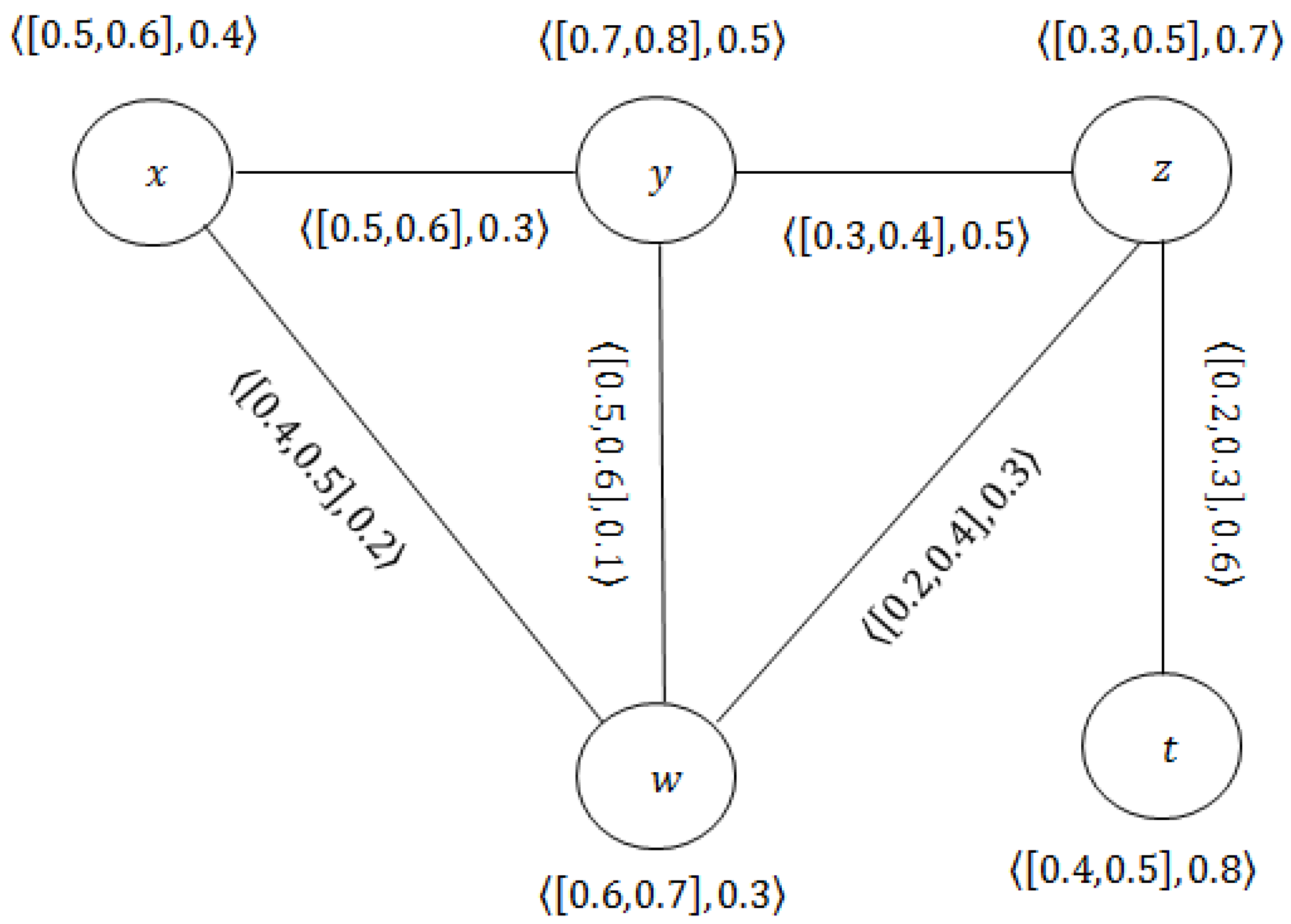
Example 1. 
Consider a CFG G as shown in Figure 1.
Here, the distance between the two nodes is as follows:
d ( x , y ) = [ 0.5 , 0.6 ] , 0.3 , d ( x , z ) = [ 0.8 , 1 ] , 0.8 , d ( x , w ) = [ 0.4 , 0.5 ] , 0.2 , d ( x , t ) = [ 0.8 , 1.2 ] , 1.1 , d ( y , z ) = [ 0.3 , 0.4 ] , 0.5 , d ( y , w ) = [ 0.5 , 0.6 ] , 0.1 , d ( y , t ) = [ 0.5 , 0.7 ] , 1.1 , d ( z , w ) = [ 0.2 , 0.4 ] , 0.3 , d ( z , t ) = [ 0.2 , 0.3 ] , 0.6 , d ( w , t ) = [ 0.4 , 0.7 ] , 0.9 .
W I α ( G ) = 0.175 + 0.12 + 0.12 + 0.16 + 0.063 + 0.21 + 0.14 + 0.036 + 0.024 + 0.096 = 1.144 W I β ( G ) = 0.288 + 0.3 + 0.21 + 0.36 + 0.16 + 0.336 + 0.28 + 0.14 + 0.075 + 0.245 = 2.394 W I γ ( G ) = 0.06 + 0.224 + 0.024 + 0.352 + 0.175 + 0.015 + 0.44 + 0.063 + 0.336 + 0.216 = 1.905 .
Therefore, W I ( G ) = [ 1.144 , 2.394 ] , 1.905 .
The Wiener index value in a cubic fuzzy subgraph does not need to be less than or equal to the original Wiener index of a CFG. This point is described in the next example.
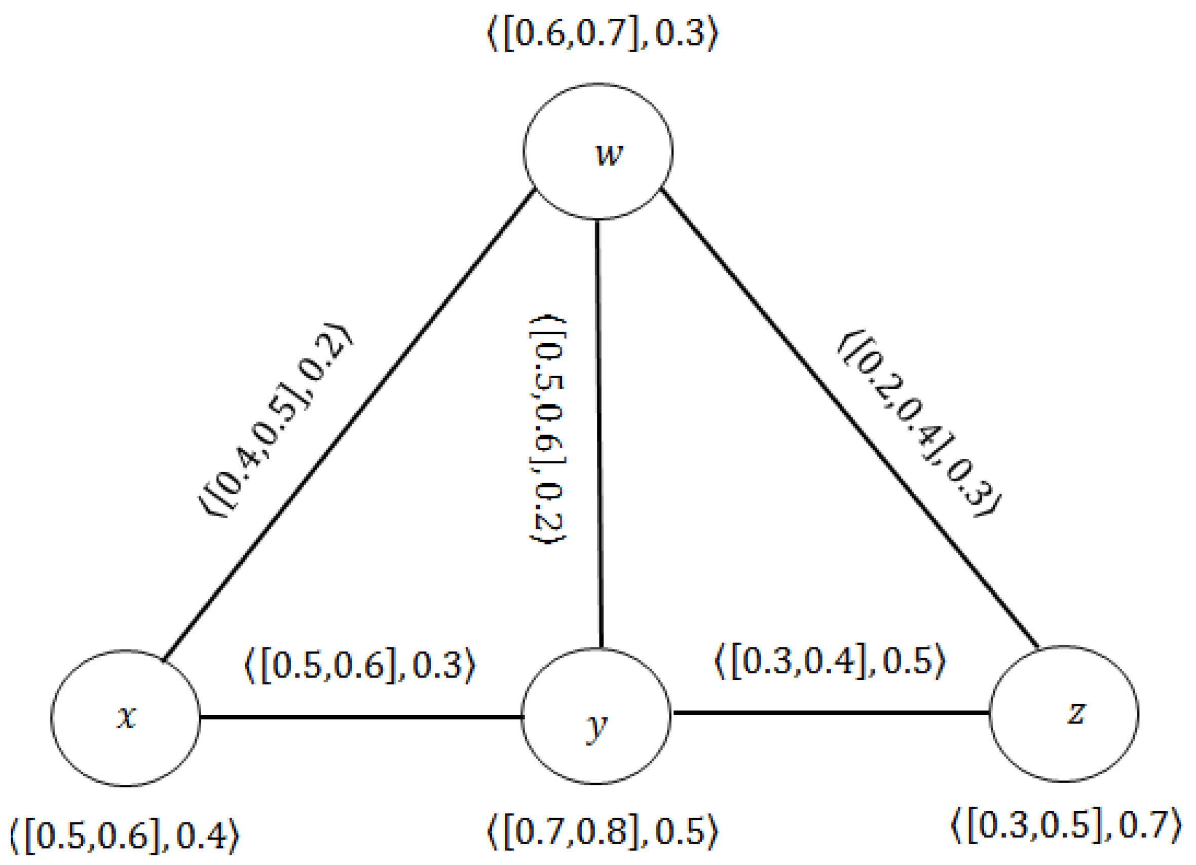
Example 2. 
Consider the cubic fuzzy subgraph H from the CFG G drawn in Figure 1. We have
W I ( H ) = [ 1.616 , 3.138 ] , 2.097 .
It is clear that
W I α ( G ) < W I α ( H ) , W I β ( G ) < W I β ( H ) , W I γ ( G ) < W I γ ( H ) .
The cubic fuzzy subgraph H is drawn in Figure 2.
It is also important to note that removing a node from a CFG also reduces the Wiener index. For example, in the CFG G , by removing the node t, the Wiener index is obtained as follows:
W I ( G t ) = [ 0.724 , 1.434 ] , 0.561 .
As can be seen, the Wiener index has decreased.
Theorem 1. 
Let G = ( X , Y ) be a CFG with α X ( z ) = β X ( z ) = γ X ( z ) = 1 for all z U and | U | = n . Let
p = min { α Y ( z w ) | z w α Y * , α ( z w ) C ( z , w ) } , q = min { β Y ( z w ) | z w β Y * , β ( z w ) C ( z , w ) } , r = min { γ Y ( z w ) | z w γ Y * , γ ( z w ) C ( z , w ) } .
Then,
W I α ( G ) p [ n ( n 1 ) | α Y * | ] , W I β ( G ) q [ n ( n 1 ) | β Y * | ] , W I γ ( G ) r [ n ( n 1 ) | γ Y * | ] .
Proof. 
Assume that ( z , w ) is any arbitrary pair of U. If z , w α Y * , then d ( z , w ) p . Therefore, there are | α Y * | unordered pairs so that d ( z , w ) P and n 2 | α Y * | are unordered node pairs so that d ( z , w ) 2 P . Then,
W I α ( G ) = d ( z , w ) | α Y * | p + n 2 | α Y * | 2 P = P [ | α Y * | + 2 n 2 2 | α Y * | ] = P [ n ( n 1 ) | α Y * | ] .
Other inequalities similar to the above argument can be proved. □
Theorem 2. 
If G = ( X , Y ) and G = ( X . Y ) are two isomorphic CFGs, then W I ( G ) = W I ( G ) .
Proof. 
Consider G and G to be two isomorphic CFGs. Thus, there is a bijective mapping f : X X so that, for every z U and z w U × U , we have
α X ( z ) = α X ( f ( z ) ) , β X ( z ) = β X ( f ( z ) ) , γ X ( z ) = γ X ( f ( z ) ) , α Y ( z w ) = α Y ( f ( z ) f ( w ) ) , β Y ( z w ) = β Y ( f ( z ) f ( w ) ) , γ Y ( z w ) = γ Y ( f ( z ) f ( w ) ) .
For all z , w U , suppose P ( z , w ) is the cubic fuzzy path that belongs to d ( z , w ) . For each cubic fuzzy edge of x y P ( z , w ) , there exists a cubic fuzzy edge f ( x ) f ( y ) in G so that
α Y ( x y ) = α Y ( f ( x ) f ( y ) ) , β Y ( x y ) = β Y ( f ( x ) f ( y ) ) , γ Y ( x y ) = γ Y ( f ( x ) f ( y ) ) .
Therefore, it can be directly said that corresponding to the cubic fuzzy path P ( z , w ) in G , there is a cubic fuzzy path P ( f ( z ) , f ( w ) ) in G so that the sum of the cubic fuzzy membership values of edges in P ( f ( z ) , f ( w ) ) is the minimum among all shortest strong cubic fuzzy paths from f ( z ) to f ( w ) . Thus,
d ( z , w ) = d ( f ( z ) , f ( w ) ) .
Then,
W I α ( G ) = z , w X α X ( z ) α X ( w ) d ( z , w ) = f ( z ) , f ( w ) X α X ( f ( z ) ) α X ( f ( w ) ) d ( f ( z ) , f ( w ) ) = W I α ( G ) .
Likewise, W I β ( G ) = W I β ( G ) and W I γ ( G ) = W I γ ( G ) . □
Corollary 1. 
Let G = ( X , Y ) be a CFG so that G * is a tree with | U | = n . Let L α ( z , w ) be the sum of the lower boundaries of the interval-valued fuzzy membership at the cubic fuzzy edges of the cubic fuzzy path P, which connects z and w. If α X ( z ) = β X ( z ) = γ X ( z ) = 1 , for all z U , then,
W I α ( G ) = z , w U , z w L α ( z , w ) , W I β ( G ) = z , w U , z w L β ( z , w ) , W I γ ( G ) = z , w U , z w L γ ( z , w ) .
This results in a CFG G where G * is a star as follows
W I α ( G ) = ( n 1 ) z w α Y * α Y ( z w ) , W I β ( G ) = ( n 1 ) z w β Y * β Y ( z w ) , W I γ ( G ) = ( n 1 ) z w γ Y * γ Y ( z w ) .
In the following, we compare the Wiener index with the connectivity index. First, let us have a reminder of the connectivity index
Definition 9. 
In the CFG ( G ) = ( X , Y ) , C I ( G ) in the following form is called the connectivity index whenever
C I ( G ) = [ C I α ( G ) , C I β ( G ) ] , C I γ ( G ) C I α ( G ) = z , w U α X ( z ) α X ( w ) C α ( z , w ) C I β ( G ) = z , w U β X ( z ) β X ( w ) C β ( z , w ) C I γ ( G ) = z , w U γ X ( z ) γ X ( w ) C γ ( z , w ) , f o r a l l z , w U .
[ C I α ( G ) , C I β ( G ) ] is denoted as the interval-valued fuzzy connectivity index and C I γ ( G ) represents the fuzzy connectivity index of G .
In the following example, we examine the comparison between the connectivity index and the Wiener index in a CFG.
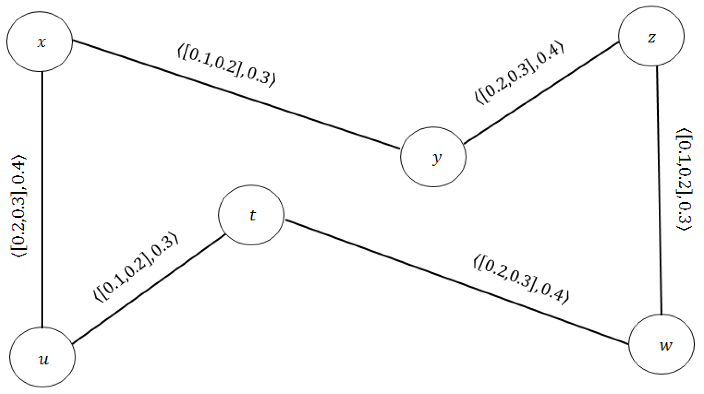
Example 3. 
Consider the CFG G drawn in Figure 3.
C ( x , y ) = [ 0.5 , 0.6 ] , 0.3 , d ( x , y ) = [ 0.5 , 0.6 ] , 0.3 , C ( x , z ) = [ 0.3 , 0.4 ] , 0.3 , d ( x , z ) = [ 0.6 , 0.9 ] , 0.5 , C ( x , w ) = [ 0.5 , 0.6 ] , 0.3 , d ( x , w ) = [ 0.4 , 0.5 ] , 0.2 , C ( y , z ) = [ 0.3 , 0.4 ] , 0.5 , d ( y , z ) = [ 0.3 , 0.4 ] , 0.5 , C ( y , w ) = [ 0.5 , 0.6 ] , 0.3 , d ( y , w ) = [ 0.5 , 0.6 ] , 0.2 , C ( z , w ) = [ 0.3 , 0.4 ] , 0.3 , d ( z , w ) = [ 0.2 , 0.4 ] , 0.3 .
After the calculations, we have
C I ( G ) = [ 0.697 , 1.296 ] , 0.463 ,
and
W I ( G ) = [ 0.694 , 1.404 ] , 0.492 .
As observed, C I α ( G ) > W I α ( G ) , C I β ( G ) < W I β ( G ) and C I γ ( G ) < W I γ ( G ) .
The results show that the values of the connectivity and Wiener indices are higher in some components and lower in others.
Proposition 1. 
If G = ( X , Y ) is a complete CFG, then
C I ( G ) = W I ( G ) .
Proof. 
Assume that G = ( X , Y ) is a complete CFG. Therefore, both nodes are connected by a cubic fuzzy edge in G . Since all cubic fuzzy edges are strong, then C ( z , w ) = d ( z , w ) . Thus,
C I ( G ) = W I ( G ) .
The above proposition immediately gives the following result.
Corollary 2. 
Let G = ( X , Y ) be a complete CFG. Let α X ( z i ) = t i , β X ( z i ) = s i and γ X ( z i ) = r i so that t 1 t 2 t n , s 1 s 2 s n and r 1 r 2 r n , for all 1 i n . Then,
W I α ( G ) = i = 1 n 1 t i 2 j = i + 1 n t j , W I β ( G ) = i = 1 n 1 s i 2 j = i + 1 n s j , W I γ ( G ) = i = 1 n 1 r i 2 j = i + 1 n r j .
Proof. 
Suppose G is a complete CFG. Moreover, let α X ( z 1 ) = t 1 , β X ( z 1 ) = s 1 and γ X ( z 1 ) = r 1 , for z 1 U . Since G is a complete CG, then
d α ( z 1 , z j ) = α X ( z 1 ) = t 1 , d β ( z 1 , z j ) = β X ( z 1 ) = s 1 , d γ ( z 1 , z j ) = γ X ( z 1 ) = r 1 , f o r a l l j > 1 .
According to the conditions, we have
α X ( z 1 ) α X ( z 2 ) α X ( z n ) , β X ( z 1 ) β X ( z 2 ) β X ( z n ) , γ X ( z 1 ) γ X ( z 2 ) γ X ( z n ) .
Therefore,
α X ( z 1 ) α X ( z j ) d α ( z 1 , z j ) = t 1 t j t 1 = t 1 2 t j , β X ( z 1 ) β X ( z j ) d β ( z 1 , z j ) = s 1 s j s 1 = s 1 2 s j , γ X ( z 1 ) γ X ( z j ) d γ ( z 1 , z j ) = r 1 r j r 1 = r 1 2 r j .
j = 2 n α X ( z 1 ) α X ( z j ) d α ( z 1 , z j ) = j = 2 n t 1 2 t j , j = 2 n β X ( z 1 ) β X ( z j ) d β ( z 1 , z j ) = j = 2 n s 1 2 s j , j = 2 n γ X ( z 1 ) γ X ( z j ) d γ ( z 1 , z j ) = j = 2 n r 1 2 r j .
Thus,
W I α ( G ) = i = 1 n 1 t i 2 j = i + 1 n t j , W I β ( G ) = i = 1 n 1 s i 2 j = i + 1 n s j , W I γ ( G ) = i = 1 n 1 r i 2 j = i + 1 n r j .
Theorem 3. 
If G = ( X , Y ) is a cubic fuzzy tree (CFT) with | U | 3 , then
C I α ( G ) W I α ( G ) , C I β ( G ) W I β ( G ) , C I γ ( G ) W I γ ( G ) .
Proof. 
Suppose G = ( X , Y ) to be a CFT. In a CFT, there is a unique strong cubic fuzzy path of P that connects each pair of nodes and is also the strongest unique cubic fuzzy path. For each z , w U , d ( z , w ) is actually the sum of the membership values of all cubic fuzzy edges that is unique in the strongest strong cubic fuzzy path, where P connecting z and w and where C ( z , w ) is the membership value of the weakest cubic fuzzy edge of P. Hence, C α ( z , w ) d α ( z , w ) , C β ( z , w ) d β ( z , w ) , C γ ( z , w ) d γ ( z , w ) . Therefore,
z , w U α X ( z ) α X ( w ) C α ( z , w ) z , w U α X ( z ) α X ( w ) d α ( z , w ) .
Thus, C I α ( G ) W I α ( G ) .
Similarly, C I β ( G ) W I β ( G ) and C I γ ( G ) W I γ ( G ) . □
In general, no direct relationship is found between the value of the Wiener index in a CFG and the value of the Wiener index after removing a node or an edge. The following example seeks further explanation.
Example 4. 
Consider the CFG G drawn in Figure 3. The value of the Wiener index after removing the y w edge is as follows
W I ( G y w ) = [ 0.699 , 1.516 ] , 0.582 .
Therefore, we have
W I α ( G y w ) = W I α ( G ) , W I β ( G y w ) > W I β ( G ) , W I γ ( G y w ) > W I γ ( G ) .
While after deleting y z , the Wiener index is as follows
W I ( G y z ) = [ 0.778 , 1.644 ] , 0.492 .
Therefore, we have
W I α ( G y z ) > W I α ( G ) , W I β ( G y z ) > W I β ( G ) , W I γ ( G y z ) = W I γ ( G ) .
On the other hand, after removing the node w, the Wiener index is W I ( G w ) = [ 0.358 , 0.748 ] , 0.459 , in which
W I α ( G w ) < W I α ( G ) , W I β ( G w ) < W I β ( G ) , W I γ ( G w ) < W I γ ( G ) .
The following definitions are used in some of the results of the Wiener index.
Definition 10. 
A cubic fuzzy edge z w of a CFG G = ( X , Y ) is named α-strong if
α Y ( z w ) > C G z w ( z w ) , β Y ( z w ) > C G z w ( z w ) , γ Y ( z w ) > C G z w ( z w ) .
z w is called β-strong if
α Y ( z w ) = C G z w ( z w ) , β Y ( z w ) = C G z w ( z w ) , γ Y ( z w ) = C G z w ( z w ) ,
and it is called δ-edge if
α Y ( z w ) < C G z w ( z w ) , β Y ( z w ) < C G z w ( z w ) , γ Y ( z w ) < C G z w ( z w ) .
It is clear that a cubic fuzzy edge is strong if it is either α-strong or β-strong.
Definition 11. 
Let G be a CFG. G is named α-saturated if at least one α-strong cubic fuzzy edge is incident at every node of z U . Moreover, G is named β-saturated if at least one β-strong cubic fuzzy edge occurs in each node.
A CFG G is named saturated if it is both α-saturated and β-saturated.
Theorem 4. 
Let G be a CFG. For z , w U , let P ( z , w ) be the cubic fuzzy path that has the minimum sum of the membership values among the shortest strong cubic fuzzy paths between z and w.
(i) 
If s t Y is a strong cubic fuzzy edge and s t is not a part of any P ( z , w ) with { z , w } { s , t } , then W I ( G s t ) W I ( G ) .
(ii) 
If s t is not a strong cubic fuzzy edge, then W I ( G s t ) = W I ( G ) .
Proof. 
( i ) Let G = ( X , Y ) be a CFG and s t Y . Let s t be a strong cubic fuzzy edge. Then, the shortest cubic fuzzy path that connects s and t is s t and d ( s , t ) = [ α Y ( s t ) , β Y ( s t ) ] , γ Y ( s t ) . If there is no cubic fuzzy path to connect s and t in G s t , then d G s t ( s , t ) < d G ( s , t ) . If s and t are connected in G s t , then there is at least one cubic fuzzy path that connects s and t with a length of at least two. Assume that s t is not part of any P ( z , w ) where z s , w t . Therefore, d G s t ( s , t ) > d G or d G s t ( s , t ) < d G according to the path P ( s , t ) in G s t . Let { s , t } { x , y } . By assuming s t is not part of P ( x , y ) , then, d G s t ( a , b ) = d G ( a , b ) . Thus, either W I ( G s t ) < W I ( G ) or W I ( G s t ) > W I ( G ) . This means W I ( G s t ) W I ( G ) .
( i i ) If s t is not a strong cubic fuzzy edge, then s t is not part of any distance from z to w for any z , w U . Therefore, removing s t from G does not change d ( z , w ) . Thus, W I ( G s t ) = W I ( G ) . □
Corollary 3. 
Let G = ( X , Y ) be a CFG so that each cubic fuzzy edge is strong. For z , w U , let P ( z , w ) be the cubic fuzzy path that has at least the sum of the membership values among the shortest strong cubic fuzzy paths between z and w. Assume that s t is not part of any P ( z , w ) where { z , w } { s , t } . Then,
(i) 
If d G s t ( s , t ) [ α Y ( s t ) , β Y ( s t ) ] , γ Y ( s t ) , then W I ( G s t ) W I ( G ) .
(ii) 
If d G s t ( s , t ) = [ α Y ( s t ) , β Y ( s t ) ] , γ Y ( s t ) , then W I ( G s t ) = W I ( G ) .
Proof. 
( i ) Since every edge in G is strong, so every edge in G s t is also strong. Therefore, d G ( s , t ) = [ α Y ( s t ) , β Y ( s t ) ] , γ Y ( s t ) . Assume that s t is not part of any P ( a , b ) with { a , b } { s , t } . Then, d G s t ( a , b ) = d G ( a , b ) . Hence, we have
W I α ( G s t ) = u , v U α Y ( u ) α Y ( v ) d α G s t ( u , v )   = u , v U α Y ( u ) α Y ( v ) d α G ( u , v ) + ( d α G s t ( s , t ) d α G ( s , t ) )   = W I α ( G ) + d α G s t ( s , t ) α Y ( s t ) .
Therefore, if d α G s t ( s , t ) > α Y ( s t ) , then W I α ( G s t ) > W I α ( G ) . Similarly, W I β ( G s t ) > W I β ( G ) and W I γ ( G s t ) > W I γ ( G ) . Thus, W I ( G s t ) > W I ( G ) .
By the same way, it can be calculated that
W I ( G s t ) < W I ( G ) .
Thus, W I ( G s t ) = W I ( G ) .
( i i ) is provable like ( i ) . □
Theorem 5. 
Let G be a cubic fuzzy cycle (CFC). Then, G is saturated CFC if and only if the following two conditions are satisfied.
(i) 
n is an even number.
(ii) 
α,β-strong cubic fuzzy edges appear consecutively on G .
Proof. 
Let G be a CFC. Therefore, G has no δ -strong cubic fuzzy edges. Suppose that G is a saturated CFC. Therefore, it is both α -saturated and β -saturated. This implies that the number of α -strong cubic fuzzy edges is equal to the number of β -strong cubic fuzzy edges. Therefore, n is an even number. Thus, each node is incident with both α , β -strong cubic fuzzy edges, which happens only when they appear consecutively on G .
Conversely, assume that G is an even CFC and α , β -strong cubic fuzzy edges appear consecutively on G . This means all the nodes are incident with exactly one α -strong and exactly with one β -strong cubic fuzzy edges. Therefore, G is both α -saturated and β -saturated. Then, G is a saturated CFC. □
Example 5. 
Consider CFC G in Figure 4, where α ( z ) = β ( z ) = γ ( z ) = 1 , for all z U . All the cubic fuzzy edges appearing alternatively on G are α,β-strong. Then, G is a saturated CFC.
Theorem 6. 
Let G = ( X , Y ) be a saturated CFC with G * = C n of length n so that each α-strong cubic fuzzy edge has a strength of [ s , t ] , r and that each β-strong cubic fuzzy edge is [ s , t ] , r . Moreover, α X ( z ) = β X ( z ) = γ X ( z ) = 1 , for all z U . Then, for m = 1 , 2 , .
W I α ( G ) = n 3 16 ( t + t ) n = 4 m n ( n 2 4 ) 16 t + n ( n 2 + 4 ) 16 t O t h e r w i s e W I β ( G ) = n 3 16 ( s + s ) n = 4 m n ( n 2 4 ) 16 s + n ( n 2 + 4 ) 16 s O t h e r w i s e W I γ ( G ) = n 3 16 ( r + r ) n = 4 m n ( n 2 4 ) 16 r + n ( n 2 + 4 ) 16 r O t h e r w i s e
Proof. 
Suppose G is a saturated CFC. Then, the cubic fuzzy edges that appear alternatively have a strength of [ s , t ] , r and [ s , t ] , r , respectively. Considering the above theorem, n is an even number. Remember that each cubic fuzzy edge of a CFC is strong. The maximum length of the node z in C n is n 2 . For k = 1 , 2 , , n 2 , we define
P k = { ( z , w ) X × X | l e n g t h o f t h e d i s t a n c e b e t w e e n z a n d w i s k . } .
There are n 2 pairs of nodes ( z , w ) so that the length of the distance z and w is n 2 . If n = 4 m , for m = 1 , 2 , , then d α ( z , w ) = n 4 ( t + t ) , for any ( z , w ) P n 2 , and n 2 4 t + n + 2 4 t , elsewhere. Therefore,
z , w P n 2 d α ( z , w ) = n 4 ( t + t ) n 2 = n 2 8 ( t + t ) n = 4 m n 2 ( n 2 4 ) t + ( n + 2 4 ) t O t h e r w i s e .
For each node z U , there are exactly two nodes at a distance of k from z. Thus, there are 2 n pairs of nodes. By avoiding repetition, there will be n pairs ( p , q ) X × X so that the length of the distance from p to q is k.
Let k be even and 1 k < n 2 . There are K 2 number of α , β -strong cubic fuzzy edges in the distance of length k from z to w. Hence, z , w P k d α ( z , w ) = n k 2 ( t + t ) .
Let k be odd and 1 k < n 2 . Consider z U and x , y are two nodes at a distance k from z. One of the distances from z of length k contains k + 1 2 α -strong cubic fuzzy edges and k 1 2 β -strong cubic fuzzy edges. The other one contain k + 1 2 β -strong cubic fuzzy edges and k 1 2 α -strong cubic fuzzy edges. Therefore,
z , w P k d α ( z , w ) = n 2 k + 1 2 t + k 1 2 t + n 2 k + 1 2 t + k 1 2 t   = n 2 ( k t + k t ) = n k 2 ( t + t ) .
Then, for n = 4 m
W I α ( G ) = n 2 8 ( t + t ) + 1 k < n 2 n k 2 ( t + t ) = ( t + t ) n 2 n 4 + 1 k < n 2 1 k = n 2 n 4 + n 2 1 × 1 + n 2 1 2 ( t + t ) = n 2 n 4 + n 2 2 n 4 ( t + t ) = n 2 n 4 + n 2 2 n 8 ( t + t ) = n 2 n 2 8 ( t + t ) = n 3 16 ( t + t ) .
where for n not a factor of 4,
W I α ( G ) = n 2 n 2 4 t + n + 2 4 t + 1 k < n 2 n k 2 ( t + t ) = n 2 n 2 4 t + n + 2 4 t + ( t + t ) n 2 1 k < n 2 1 k = n 2 n 2 4 t + n + 2 4 t + n 2 n 2 1 × 1 + n 2 1 2 ( t + t ) = n 2 n 2 4 t + n + 2 4 t + n 2 n ( n 2 ) 8 ( t + t ) = n ( n 2 4 ) 16 t + n ( n 2 + 4 ) 16 t .
W I β ( G ) and W I α ( G ) are also proved according to the above method. □

4. Application

Chemistry is concerned with how subatomic particles bond to form atoms. In addition, in chemistry, there is a focus on how atoms bond to form molecules. In a molecular graph, all atoms and chemical bonds are labeled. This labeled graph is used in the physical and chemical predictions of a compound, quantitatively and qualitatively describing the chemical structures, structural features and activities related to topological indices.
One of the characteristics of an atom that plays a very important role in the properties of compounds is the radius of the atom and its electronegative properties. Bond length and bond energy are also the important features of a bond. Electronegativity is the degree to which an atom in a molecule tends to attract a pair of bonding electrons to itself. The Pauling electronegative relative scale is the most common scale based on the experimental values of bond energies. The radius of an atom indicates its effective size, when measured in combination with other atoms. In fact, determining the atomic radius is difficult because there is uncertainty, so a constant atomic radius cannot be determined for an atom. The radius of a single atom is in the range of 30 to 300 pm or between 0.3 and 3 angstroms.
In molecular geometry, bond length or bond distance is defined as the average distance between two atoms bond in a molecule. The length of the bond depends on the order of the bond. When more electrons are present in a bond, we have a shorter bond. The length of the bond also inversely depends on the strength of the bond and the dissociation energy of the bond. The stronger the bond, the shorter it will be when all the factors are the same.
Until 1920, chemists did not think that molecules with a molecular weight greater than a thousand existed. Until a German chemist named Hermann Staudinger challenged this theory by studying the composition of substances such as rubber and cellulose. Contrary to popular belief, he suggested that these compounds were made up of macromolecules of 10,000 atoms or more. He formulated a polymer structure for rubber based on a repeated isoprene unit (called a monomer) and was awarded the 1953 Nobel Prize.
Monomers are actually the building blocks of polymer molecules. In simpler terms, one monomer is added to another to form a polymer chain. This process is called polymerization. Monomers are essential elements for many industries and have a variety of applications, from food packaging to coatings for vehicles and home appliances. Monomers provide selectivity, quality and compatibility, dispersion and emulsions for a variety of adhesives, coatings, inks, woven and nonwoven textiles, plastics and polymers and highly absorbent products
In this study, three monomers were examined, which included the molecules drawn in Figure 5.
A CFG can be useful in examining some properties of molecules. For this purpose, each of the above molecules was considered as a CFG. The atomic radius and electronegative number of some atoms along with their cubic fuzzy values are given in Table 1. In this table, the atomic radius with an interval-valued fuzzy number with a difference of 0.01 from the center of the interval and the electronegative number of each atom is shown with a fuzzy number, which is the ratio of the number of each atom to four. The values for the length and energy of some chemical bonds between atoms, along with the cubic fuzzy values for each of them, are presented in Table 2. In this table, the cubic fuzzy values of each bond are calculated in relation to a maximum of 300 and 1000 pm.
The Wiener index of each molecule is calculated in Table 3.
Looking at Table 3, it can be concluded that by substituting H atoms in ethene with F atoms, the bond energy increased tremendously because its fuzzy Wiener index increased more than that of other molecules. Polymers based on a C 2 F 4 molecule seem to have a good level of strength. In addition, a decrease in the interval-valued Wiener index in C 2 F 4 compared to C 2 H 4 means a decrease in the bond length of this molecule and an increase in its melting point. The available data confirmed the results obtained.
The results for the C 2 H 3 Cl molecule were similar as those of C 2 H 4 , except for the fact that the interval-valued Wiener index in this molecule was higher than in the other two molecules, which provided a greater bond length between its atoms. It seems that by replacing Cl with H, we saw an increase in the length and energy of the bond in the molecule. The study of this issue in C 2 HCl 3 molecule drawn in Figure 6 with Wiener index [ 0.70911 , 0.87615 ] , 2.775757 confirmed this point.
A major part of the properties of these molecules depends on the two intermediate atoms. To confirm this, we calculated the Wiener index in N 2 H 4 as shown in Figure 7.
The Wiener index of this molecule was [ 0.273262 , 0.364736 ] , 0.565568 , which indicated a decrease for all components values compared to the above molecules.

5. Conclusions

A topological index is a real number based on the distance of nodes in a graph. Among these indices, the Wiener index was the first defined index to be used as a tool for modeling chemical, pharmacological and other molecular properties. The Wiener index is one of the defining criteria in fuzzy graphs, where we are faced with uncertain values. It is even more important to know that we are dealing with a fuzzy graph that has both fuzzy membership and interval-valued membership, that is, a CFG. Determining the Wiener index in a CFG is directly related to the bond strength between nodes. In this paper, by extending the Wiener index in fuzzy graphs to cubic graphs, we presented a new definition of the Wiener index with both numerical and interval values. Some of its basic properties were investigated, including determining the value of the Wiener index in certain CFGs, changing the Wiener index by removing one node or an edge of the CFG and the formula for the value of the Wiener index in a saturated CFC. The results showed that the value of the Wiener index was not always associated with a decrease or increase. In some cases, the value of the fuzzy Wiener index increased while the value of the interval-valued Wiener index decreased. Using the results obtained in determining the Wiener index of some monomer molecules, an application of this index in the study of the properties of polymer molecules was presented. Studying the properties of the connectivity index and the average connectivity index will be future work.

Author Contributions

X.S., A.A.T. and S.H.S.; methodology, X.S., M.A. and A.A.T.; formal analysis, X.S. and A.A.T.; investigation, X.S., M.A., A.A.T. and S.H.S.; data curation, X.S., M.A. and S.H.S.; writing—original draft preparation, X.S. and A.A.T.; writing—review and editing, X.S., M.A., A.A.T. and S.H.S.; visualization, X.S., M.A., A.A.T. and S.H.S.; funding acquisition, X.S. All authors have read and agreed to the published version of the manuscript.

Funding

This work was supported by the National Key R&D Program of China (grant 2019YFA0706402), and the National Natural Science Foundation of China under grants 62172302, 62072129 and 61876047.

Institutional Review Board Statement

Not applicable.

Informed Consent Statement

Not applicable.

Data Availability Statement

Not applicable.

Conflicts of Interest

The authors declare no conflict of interest.

References

  1. Wiener, H. Structural determination of paraffin boiling points. J. Am. Chem. Soc. 1947, 69, 17–20. [Google Scholar] [CrossRef]
  2. Zadeh, L.A. Information and control. Fuzzy Sets 1965, 8, 338–353. [Google Scholar]
  3. Rosenfeld, A. Fuzzy Graphs, Fuzzy Sets and Their Applications; Academic Press: New York, NY, USA, 1975; pp. 77–95. [Google Scholar]
  4. Mordeson, J.N.; Chang-Shyh, P. Operations on fuzzy graphs. Inf. Sci. 1994, 79, 159–170. [Google Scholar] [CrossRef]
  5. Akram, M. Bipolar fuzzy graphs with applications. Knowl.-Based Syst. 2013, 39, 1–8. [Google Scholar] [CrossRef]
  6. Atanassov, K.T. Intuitionistic fuzzy sets. In Physica; Springer: Berlin/Heidelberg, Germany, 1999; pp. 1–137. [Google Scholar]
  7. Akram, M.; Davvaz, B. Strong intuitionistic fuzzy graphs. Filomat 2012, 26, 177–196. [Google Scholar] [CrossRef] [Green Version]
  8. Akram, M.; Karunambigai, M.G.; Palanivel, K.; Sivasankar, S. Balanced bipolar fuzzy graphs. J. Adv. Res. Pure Math. 2014, 6, 58–71. [Google Scholar]
  9. Akram, M.; Dudek, W.A. Intuitionistic fuzzy hypergraphs with applications. Inf. Sci. 2013, 218, 182–193. [Google Scholar] [CrossRef]
  10. Borzooei, R.A.; Rashmanlou, H. New concepts of vague graphs. Int. J. Mach. Learn. Cybern. 2016, 8, 1081–1092. [Google Scholar] [CrossRef]
  11. Talebi, A.A.; Rashmanlou, H.; Sadati, S.H. New concepts on m-polar interval-valued intuitionistic fuzzy graph. TWMS J. Appl. Eng. Math. 2020, 10, 808–816. [Google Scholar]
  12. Talebi, A.A.; Rashmanlou, H.; Sadati, S.H. Interval-valued Intuitionistic Fuzzy Competition Graph. J. Mult.-Valued Log. Soft Comput. 2020, 34, 335–364. [Google Scholar]
  13. Kosari, S.; Rao, Y.; Jiang, H.; Liu, X.; Wu, P.; Shao, Z. Vague graph structure with application in medical diagnosis. Symmetry 2020, 12, 1582. [Google Scholar] [CrossRef]
  14. Rao, Y.; Kosari, S.; Shao, Z. Certain properties of vague graphs with a novel application. Mathematics 2020, 8, 1647. [Google Scholar] [CrossRef]
  15. Rao, Y.; Kosari, S.; Shao, Z.; Cai, R.; Xinyue, L. A study on domination in vague incidence graph and its application in medical sciences. Symmetry 2020, 12, 1885. [Google Scholar] [CrossRef]
  16. Shi, X.; Kosari, S. Certain Properties of Domination in Product Vague Graphs With Novel Application in Medicine. Front. Phys. 2021, 9, 3–85. [Google Scholar] [CrossRef]
  17. Kou, Z.; Kosari, S.; Akhoundi, M. A Novel Description on Vague Graph with Application in Transportation Systems. J. Math. 2021, 2021, 4800499. [Google Scholar] [CrossRef]
  18. Rao, Y.; Kosari, S.; Shao, Z.; Qiang, X.; Akhoundi, M.; Zhang, X. Equitable Domination in Vague Graphs With Application in Medical Sciences. Front. Phys. 2021, 37, 635642. [Google Scholar] [CrossRef]
  19. Shao, Z.; Kosari, S.; Rashmanlou, H.; Shoaib, M. New concepts in intuitionistic fuzzy graph with application in water supplier systems. Mathematics 2020, 8, 1241. [Google Scholar] [CrossRef]
  20. Zeng, S.; Shoaib, M.; Ali, S.; Abbas, Q.; Nadeem, M.S. Complex vague graphs and their application in decision-making problems. IEEE Access 2020, 8, 174094–174104. [Google Scholar] [CrossRef]
  21. Zeng, S.; Shoaib, M.; Ali, S.; Smarache, F.; Rashmanlou, H.; Mofidnakhaei, F. Certain properties of single-valued neutrosophic graph with application in food and agriculture organization. Int. J. Comput. Intell. Syst. 2021, 14, 1516–1540. [Google Scholar] [CrossRef]
  22. Ali, S.; Kousar, M.; Xin, Q.; Pamučar, D.; Hameed, M.S.; Fayyaz, R. Belief and possibility belief interval-valued N-soft set and their applications in multi-attribute decision-making problems. Entropy 2021, 23, 1498. [Google Scholar] [CrossRef]
  23. Jun, Y.B.; Kim, C.S.; Yang, K.O. Cubic sets. Ann. Fuzzy Math. Inform. 2012, 4, 83–98. [Google Scholar]
  24. Jun, Y.B.; Smarache, F.; Kim, C.S. Neutrosophic cubic sets. New Math. Nat. Comput. 2017, 13, 41–54. [Google Scholar] [CrossRef] [Green Version]
  25. Jun, Y.B.; Song, S.Z.; Kim, S.J. Cubic interval-valued intuitionistic fuzzy sets and their application in BCK/BCI-algebras. Axioms 2018, 7, 7. [Google Scholar] [CrossRef] [Green Version]
  26. Jun, Y.B.; Lee, K.J.; Kang, M.S. Cubic structures applied to ideals of BCI-algebras. Comput. Math. Appl. 2011, 62, 3334–3342. [Google Scholar] [CrossRef] [Green Version]
  27. Khan, M.; Jun, Y.B.; Gulistan, M.; Yaqoob, N. The generalized version of Jun’s cubic sets in semigroups. J. Intell. Fuzzy Syst. 2015, 28, 947–960. [Google Scholar] [CrossRef]
  28. Ali, A.; Jun, Y.B.; Khan, M.; Shi, F.G.; Anis, S. Generalized cubic soft sets and their applications to algebraic structures. Ital. J. Pure Appl. Math. 2015, 35, 393–414. [Google Scholar]
  29. Senapati, T.; Jun, Y.B.; Muhiuddin, G.; Shum, K.P. Cubic intuitionistic structures applied to ideals of BCI-algebras. Analele Stiintifice Ale Univ. Ovidius-Constanta-Ser. Mat. 2019, 27, 213–232. [Google Scholar] [CrossRef] [Green Version]
  30. Muhiuddin, G.; Takallo, M.M.; Jun, Y.B.; Borzooei, R.A. Cubic graphs and their application to a traffic flow problem. Int. J. Comput. Intell. Syst. 2020, 13, 1265–1280. [Google Scholar] [CrossRef]
  31. Rashmanlou, H.; Muhiuddin, G.; Amanathulla, S.K.; Mofidnakhaei, F.; Pal, M. A study on cubic graphs with novel application. J. Intell. Fuzzy Syst. 2021, 40, 89–101. [Google Scholar] [CrossRef]
  32. Jiang, H.; Talebi, A.A.; Shao, Z.; Sadati, S.H.; Rashmanlou, H. New Concepts of node Covering in Cubic Graphs with Its Applications. Mathematics 2022, 10, 307. [Google Scholar] [CrossRef]
  33. Mathew, S.; Sunitha, M.S. Node connectivity and arc connectivity of a fuzzy graph. Inf. Sci. 2010, 180, 519–531. [Google Scholar] [CrossRef]
  34. Mathew, S.; Sunitha, M.S. Cycle connectivity in fuzzy graphs. J. Intell. Fuzzy Syst. 2013, 24, 549–554. [Google Scholar] [CrossRef]
  35. Binu, M.; Mathew, S.; Mordeson, J.N. Wiener index of a fuzzy graph and application to illegal immigration networks. Fuzzy Set Syst. 2019, 384, 132–147. [Google Scholar]
  36. Binu, M.; Mathew, S.; Mordeson, J.N. Connectivity index of a fuzzy graph and its application to human trafficking. Fuzzy Set Syst. 2019, 360, 117–136. [Google Scholar]
  37. Binu, M.; Mathew, S.; Mordeson, J.N. Cyclic connectivity index of fuzzy graphs. IEEE Trans. Fuzzy Syst. 2020, 29, 1340–1349. [Google Scholar] [CrossRef]
  38. Lee, H.; Chen, X.G.; Sohn, M.Y. A Note on “Wiener Index of a Fuzzy Graph and Application to Illegal Immigration Networks”. Appl. Sci. 2021, 12, 304. [Google Scholar] [CrossRef]
  39. Fang, J.; Nazeer, I.; Rashid, T.; Liu, J.B. Connectivity and Wiener index of fuzzy incidence graphs. Math. Probl. Eng. 2021, 2021, 6682966. [Google Scholar] [CrossRef]
  40. Poulik, S.; Ghorai, G. Certain indices of graphs under bipolar fuzzy environment with applications. Soft Comput. 2020, 24, 5119–5131. [Google Scholar] [CrossRef]
  41. Mandal, S.; Pal, M. Connectivity Index of M-Polar Fuzzy Graph with Application. Res. Sq. 2021. [Google Scholar] [CrossRef]
  42. Mordeson, J.N.; Mathew, S.; Malik, D.S. Fuzzy Graph Theory with Applications to Human Trafficking; Springer: Berlin/Heidelberg, Germany, 2018; p. 365. [Google Scholar]
Figure 1. A CFG G .
Figure 1. A CFG G .
Symmetry 14 02623 g001
Figure 2. Cubic fuzzy subgraph H of G .
Symmetry 14 02623 g002
Figure 3. The comparison between C I ( G ) and W I ( G ) in a CFG G .
Symmetry 14 02623 g003
Figure 4. A saturated CFC.
Symmetry 14 02623 g004
Figure 5. Three types of monomers from the alkenes group.
Symmetry 14 02623 g005
Figure 6. Molecular structure of trichloroethene.
Symmetry 14 02623 g006
Figure 7. Molecular structure of hydrazine.
Symmetry 14 02623 g007
Table 1. Cubic fuzzy values of atoms.
AtomsAtomic Radius (pm)Electronegative NumberCubic Fuzzy Number
H53 2.20 [ 0.16 , 0.18 ] , 0.13
C65 2.55 [ 0.20 , 0.22 ] , 0.63
N55 3.04 [ 0.17 , 0.19 ] , 0.76
F41 3.98 [ 0.12 , 0.14 ] , 0.99
Cl78 3.16 [ 0.25 , 0.27 ] , 0.79
Table 2. Cubic fuzzy values of bonds.
BondsLength (pm)Energy (kJ/mol)Cubic Fuzzy Number
C–H109413 [ 0.35 , 0.37 ] , 0.41
C–F135488 [ 0.44 , 0.46 ] , 0.48
C–Cl17778 [ 0.58 , 0.60 ] , 0.07
C=C134614 [ 0.43 , 0.45 ] , 0.61
N–H101391 [ 0.32 , 0.34 ] , 0.39
N=N141170 [ 0.46 , 0.48 ] , 0.17
Table 3. The Wiener index values of molecules.
WI ( G ) C 2 H 4 C 2 F 4 C 2 H 3 Cl
W I α ( G ) 0.313392 0.24376 0.426956
W I β ( G ) 0.412452 0.334036 1.171176
W I γ ( G ) 0.834961 12.195765 1.302109
Publisher’s Note: MDPI stays neutral with regard to jurisdictional claims in published maps and institutional affiliations.

