Article

Novel Complex Pythagorean Fuzzy Sets under Aczel–Alsina Operators and Their Application in Multi-Attribute Decision Making

1
Department of Statistics, Zhejiang University City College, Hangzhou 310015, China
2
Department of Mathematics, Riphah International University Lahore, Lahore 5400, Pakistan
*
Authors to whom correspondence should be addressed.
Symmetry 2023, 15(1), 68; https://doi.org/10.3390/sym15010068
Submission received: 17 November 2022 / Revised: 4 December 2022 / Accepted: 19 December 2022 / Published: 26 December 2022
(This article belongs to the Special Issue Research on Fuzzy Logic and Mathematics with Applications II)

Abstract

:
Aggregation operators (AOs) are utilized to overcome the influence of uncertain and vague information in different fuzzy environments. A multi-attribute decision-making (MADM) technique plays a vital role in several fields of different environments such as networking analysis, risk assessment, cognitive science, recommender systems, signal processing, and many more domains in ambiguous circumstances. In this article, we elaborated the notion of Aczel–Alsina t-norm (TNM) and t-conorm (TCNM) under the system of complex Pythagorean fuzzy (CPyF) sets (CPyFSs). Some basic operational laws of Aczel–Alsina TNM and TCNM are established including Aczel–Alsina sum, product, scalar multiplication, and power operations based on CPyFSs. We established several AOs of CPyFSs such as CPyF Aczel–Alsina weighted average (CPyFAAWA), and CPyF Aczel–Alsina weighted geometric (CPyFAAWG) operators. The proposed CPyFAAWA and CPyFAAWG operators are symmetric in nature and satisfy the properties of idempotency, monotonicity, boundedness and commutativity. To solve an MADM technique, we established an illustrative example to select a suitable candidate for a vacant post in a multinational company. To see the advantages of our proposed AOs, we compared the results of existing AOs with the results of newly established AOs.

1. Introduction

The purpose of the MADM technique is to categorize and deal with problems using a variety of different criteria. The MADM methodology has become increasingly popular among decision-makers as a consequence of its numerous applications in a variety of disciplines, including operation research, engineering technology management science, etc., through collecting the information into a single useful form, AOs are essential in helping to address all MADM issues. The decision-makers in real decision making categorize the alternatives using a variety of evaluation techniques, such as interval numbers or crisp numbers. Due to the growing uncertainty involved and the ambiguities of data, it has become more challenging for decision makers to solve decision-making problems using precise numerical values. Zadeh [1] introduced the novel idea of the fuzzy set (FS) in 1965, by launching the membership value (MV), whose range lies between 0 and 1 , to address this issue. In order to tackle decision-making problems involving uncertainties and ambiguities in the data more precisely than a crisp set, Zadeh’s creation of the FS gives decision making a plate form. To overcome the decision-making difficulties, Atanassov [2] enlarged the concepts of FS in the form of intuitionistic FS (IFS) in which the sum of the MV and the non-membership value (NMV) lies on interval 0 , 1 . i.e., 0 Π + Ξ 1 , where Π 0 , 1 represents MV and Ξ 0 , 1 represents NMV in an IFSs. In some scenarios, when IFSs failed to deal with uncertain and vague information in fuzzy system, Yager [3] provided an innovative idea of IFS in the form of Pythagorean FS (PyFS) in such a way that the sum of the square of MV and NMV lies on interval 0 , 1 , i.e.,   0 Π 2 + Ξ 2 1 . Several researchers have plenty of commentary the above-discussed fuzzy environment. Adlassnig [4] generalized the theory of FSs to formalize the uncertain information under the system of medical diagnosis. Atanassov [5] also explored concepts of IFS in the framework of interval-valued IFS (IVIFS) with upper and lower cases of MV and NMV of an IVIFS. Mohd and Abdullah [6] proposed a study of several similarity measured distances based on PyFSs.
It has been determined that the MCDM concerns were resolved, as the above current research in FS, IFS, and extended sets, such as PyFSs settings, are only capable of handling the vagueness and ambiguity of the data. All of these models are unable to address the lack of historical knowledge and data sensitivity. However, a complex data collection can handle both the periodicity and the uncertainty of the data at the same time. To deal with these circumstances, Ramot et al. [7,8] proposed the idea of a complex fuzzy set (CFS). They suggested that Π e i α Π , whose range is expanded from unit disc to a complex plane, where   Π 0 ,   1 represents the MV of an amplitude term of a CFS and α Π 0 ,   2 π represents MV of phase terms of a CFS. Alkouri and Salleh [9] extended the theory of CFSs in the form of complex IFS (CIFS), having two aspects of MV and NMV in such a way that Π e i α , Ξ e π i β ,   i = 1 . A CIFS satisfied the conditions   0 Π + Ξ 1 and 0 α + β 2 π , where Π 0 , 1 and Ξ 0 , 1 represent the MV and NMV of amplitude terms, respectively. In the same way, α 0 , 2 π and β 0 , 2 π represents the MV and NMV of phase terms, respectively. Ullah et al. [10] developed an innovative concept of CIFS in the framework of complex PyFS (CPyFSs), and relaxed the condition of CIFS with the square of amplitude and phase terms of MV and NMV, respectively. Riaz and Hashmi [11] provided a new extension of FSs in the form of linear Diophantine FS to handle vagueness and uncertainty in the fuzzy system. Akram and Naz [12] introduced an innovative idea of PyFS in the framework of CPyFS to cope with uncertain information under an MADM approach. Khan et al. [13] utilized the theory of complex T-SFSs to provide some new averaging and geometric operators based on power aggregation tools. Ali et al. [14] explored the idea of complex q-ROFS and developed some new AOs to solve real life problem using an MADM technique. Mahmood [15] worked on a bipolar soft set to cope with uncertain and ambiguous information. We also studied some basic notions of the fuzzy environment related to our research work, which are not discussed in the above paragraphs, seen in [15,16,17,18].
AOs are essential tools to cope with uncertain and vague information in different fuzzy environments. Several researchers worked on a distinct model of classical set theory and fuzzy systems. We studied some AOs developed by Xu [19] in the form of weighted averaging operators and some special cases based on IFSs. Wei [20] invented some AOs in the form of induced weighted geometric operators, and ordered weighted geometric operators and hybrid weighted geometric operators. Peng and Yuan [21] explored some inequalities and invented some AOs of PyF value (PyFV) in the form of generalized weighted averaging operators. Akram et al. [22] explored the idea of interval valued T-FSs based on a Bonferroni mean operator, and established an MADM technique under the solar system. Khan et al. [23] extended the concepts of spherical FSs (SFSs) and introduced some new AOs of SFSs based on Dombi aggregation tools. Rahman et al. [24] presented a list of new AOs of PyFSs-like weighted averaging, and weighted geometric operators with some basic deserved characteristics. Mahmood et al. [25] presented some new AOs, an innovative concept of PyFS in the form of complex PyFS (CPyFS), to overcome the influence of vague and ambiguous information under the CPyFS system. Liu et al. [26] explored the concepts of IFS to deal with vague information, and also developed a list of new AOs by utilizing the concepts of Maclaurin symmetric mean operators. Ullah [27] utilized the concepts of Maclaurin symmetric mean operators and developed a list of new AOs based on picture FS (PFS). Akram et al. [28] provided some new AOs of PyFS and also studied an MADM technique to complete a selection process for the textile industry. Chen [29] developed new approaches by utilizing the innovative concept of prioritized AOs based on IVIFS. Liu and Wang [30] presented a list of new AOs by using the concepts of Archimedean Bonferroni tools under the system of q-rung orthopair FS (q-ROFS) to solve a real-life problems based on MADM techniques. Hussain et al. [31] explored a list of new AOs and gave an illustrative example to solve an MADM problem for the selection of suitable tourism destinations. Garg [32] developed a series of new AOs with entropy weight vectors based on IF information. Akram and Shahzadi [33] worked on a new concept of Yager AOs and gave an MADM technique under the system of q-ROFS. Jan et al. [34] introduced some new AOs under the system of linguistic cubic information to solve an MADM technique. Yang et al. [35] explored an innovative idea of the TOPSIS method and developed some new aggregation tools of Fermatean fuzzy integrated weighted distance to process fuzzy information. Mahmood [18] modified traditional Maclaurin symmetric mean operators and developed a list of new AOs in the environment of a bipolar complex fuzzy system. Ullah et al. [36] utilized the concepts of T-spherical FSs (T-SFSs) and provided some AOs of T-SFSs to solve an MADM problem.
Menger [37] introduced a new concept of triangular norms based on probabilistic metric space in 1942. Klement [38] presented some new aggregated tools by utilizing the theory of t-norm (TNM) and t-conorm (TCNM) in different fuzzy information. To aggregate the information in numerous mathematical structures, a series of triangular norms were constructed. Information aggregation is critical for solving various MADM issues. Many different types of TN and TCN have been applied to the increase in the average and geometric aggregation process. The invented TNMs and TCNMs are the Lukasiewicz TNM and TCNM [39], drastic TNM and TCNM [40], nilpotent TNM and TCNM [41], Frank TNM and TCNM [42], Archimedean TNM and TCNM [43], Einstein TNM and TCNM [44], probabilistic TNM and TCNM [45] and Dombi TNM and TCNM [46]. Recently Mahmood et al. [47] proposed a new idea to cope with unpredictable and vague information by developing a list of AOs based on the Frank TNM and TCNM under a system of interval-valued picture FSs. Liu [48] explored the theory of algebraic and Einstein AOs in the form of Hamacher AOs based on IVIF information. Garg [49] generated the concepts of PyFSs and developed some new approaches to geometric AOs by utilizing the operations of the Einstein TNM and TCNM in the environment of PyFSs. Liu and Wang [30] proposed a list of new AOs by using the fundamental operations of Archimedean Bonferroni operators under the system of q-ROFSs with an MADM technique. We also studied existing research work seen in the references [50,51].
Aczel and Alsina [52] discovered some more reliable and flexible TNMs and TCNMs like the Aczel–Alsina TNM (AA-TNM) and the Aczel–Alsina TCNM (AA-TCNM) in 1982. We can overcome the impact of unreasonable and unpredictable information in different fuzzy environments. Babu and Ahmed [53] worked on several TNMs and TCNMs to classify the best TNM and TCNM from a family of TNMs and TCNMs. After evaluation, they found that AA-TNM and AA-TCNM are more suitable aggregation tools than other ones. To see the advantages and benefits of AA-TNM and AA-TCNM, several researchers utilized these aggregation tools in their research works. Recently, Senapati et al. [54] explored the concepts of AA-TNM and AA-TCNM and established an illustrative example to solve an MAMD technique under the system of IFSs. Senapati et al. [55] also generalized the theory of AA-TNM and AA-TCNM and gave a list of new AOs based on IVIFSs. Naeem et al. [56] enlarged the concepts of AA-TNM and AA-TCNM with more extensive information in the framework of picture FSs (PFSs). Hussain et al. [57] enlarged the concepts of T-SFSs and developed some new AOs using the basic operations of AA-TNM and AA-TCNM. All of the aforementioned invented AOs to handle two tuple information; there is a chance of losing information during the aggregation process, whereby a decision maker cannot obtain original results for the decision’s purpose. A CPyFS contains more information than FSs, IFSs and PyFSs. Keeping in mind the significance of CPyFSs, we developed some innovative concepts of AA-TNM and AA-TCNM within the framework of CPyFSs. The main contributions of this article are in the following forms:
(1)
We presented some new AOs and fundamental operational laws of CPyFSs. We also generalized the basic idea of Aczel–Alsina TNM and TCNM, with their operational laws and illustrative examples.
(2)
By using the operational laws of Aczel–Alsina TNM and TCNM, we developed a list of new AOs like the CPyFAAWA operator and verified invented AOs with some deserved properties.
(3)
Furthermore, we also established the CPyFAAWAG operator based on the defined fundamental operational laws of Aczel–Alsina TNM and TCNM.
(4)
To find the feasibility and reliability of our invented methodologies, we explored some special cases, like CPyFAA ordered weighted (CPyFAAWAG), average (CPyFAAWAG) and CPyFAAOW geometric (CPyFAAOWG) operators, CPyFAA hybrid weighted (CPyFAAHW), average (CPyFAAHWA) and CPyFAAHW geometric (CPyFAAOWG) operators with some basic properties.
(5)
By utilizing our invented approaches, we solved an MADM technique. We established an illustrative example to select a suitable candidate for a vacant post at a multinational company.
(6)
To analyse the effectiveness of different parametric values of   on the results of our proposed approaches, we discussed an influence study.
(7)
We checked the reliability and flexibility of our invented approaches, by comparing the results of existing AOs with the results of our discussed technique.
The structure of this manuscript is presented as follows and also displayed in the Figure 1: in Section 1, we thoroughly overviewed all previous history of our research work; in Section 2, we recall the notions of CFSs, CPyFSs and fundamental operations of CPyFSs. In Section 3, we studied the concepts of some existing AOs under the different environments of fuzzy systems. In Section 4, we introduced innovative concepts of Aczel–Alsina operations under the system of CPyF information. In Section 5, we developed several AOs of CPyFAAWA operators, and some special cases are also present here. In Section 6, we enlarged the idea of CPyFSs and introduced some AOs in the form of CPyFAAWG operators with some deserved characteristics. In Section 7, we solved an MADM technique to find the reliability and flexibility of our invented AOs, and we gave an illustrative example to select a suitable candidate for a multinational company. In Section 8, we studied the advantages and verified our invented AOs by comparing the results of existing AOs with the results of our invented AOs. In Section 9, we summarized the whole article in a single paragraph.

2. Preliminaries

We recall the notions of CFS and CPyFSs, and also discussed some basic operations of CPyFSs. Further, we studied the notion of score and accuracy function to compare CPyF values (CPyFVs).
Definition 1
([7]). Consider to be a non-empty set, and a CFS Λ is defined as:
Λ = x ,   Π Λ ϰ e 2 π i α Λ ϰ : x ,   i = 1
where Π Λ ϰ   0 ,   1 and   α Λ ϰ   0 ,   1 represents the membership value (MV) of amplitude terms and phase terms of   Λ , respectively. A CFS must satisfy the condition:
0   Π Λ ϰ   1   and   0 α Λ ϰ   1 .
In the following Table 1, we define the symbols and their meanings.
Definition 2
([9]). A CPyFS Λ on a is defined as:
Λ =   Π Λ ϰ e 2 π i α Λ ϰ , Ξ Λ ϰ e 2 π i β Λ ϰ : x   ,   i = 1  
where Π Λ ϰ   0 ,   1 and   α Λ ϰ   0 ,   1 represents amplitude terms and phase terms of MV, respectively. Similarly   Ξ Λ ϰ   0 ,   1 and   β Λ ϰ   0 ,   1 represents amplitude and phase terms of NMV, respectively. A CPyFS must satisfy these conditions:
0   Π Λ 2 x + Ξ Λ 2 ϰ   1   and   0 α Λ ϰ 2 + β Λ ϰ 2   1
For the sake of convenience, the pair Λ = Π ϰ e 2 π i α ϰ , Ξ ϰ e 2 π i β ϰ is known as CPyFV.
Definition 3
([31]). Let Ω = Π ϰ e 2 π i α ϰ , Ξ ϰ e 2 π i β ϰ be a CPyFV; then, the score function R ˘ Ω of CPyFVs is given as:
R ˘ Ω = Π ϰ 2 Ξ ϰ 2 + α ϰ 2 β ϰ 2 2
and the accuracy function is given as:
A ˘ Ω = Π ϰ 2 + Ξ ϰ 2 + α ϰ 2 + β ϰ 2 2
where R ˘   Ω   1 ,   1   and A ˘   Ω     0 ,   1 .
Definition 4
([33]). Let Ω 1 = ( Π 1 ( ϰ ) e 2 π i ( α 1 ( ϰ ) ) , Ξ 1 ( ϰ ) e 2 π i ( β 1 ( ϰ ) ) ) and Ω 2 = ( Π 2 ( ϰ ) e 2 π i ( α 2 ( ϰ ) ) , Ξ 2 ( ϰ ) e 2 π i ( β 2 ( ϰ ) ) ) be two CPyFVs. Then
i. 
If   R ˘ ( Ω 1 ) < R ˘ ( Ω 2 ) ,   then  Ω 1 < Ω 2 ,
ii. 
If   R ˘ ( Ω 1 ) = R ˘ ( Ω 2 ) ,   then we need to find out the accuracy function:
i. 
If   A ˘ ( Ω 1 ) < A ˘ ( Ω 2 ) ,   then  Ω 1 < Ω 2 ,
ii. 
If   A ˘ ( Ω 1 ) = A ˘ ( Ω 2 ) ,   then  Ω 1 = Ω 2 .
Definition 5
([32]). Let  Ω 1 = Π 1 ϰ e 2 π i α 1 ϰ , Ξ 1 ϰ e 2 π i β 1 ϰ  and  Ω 2 = Π 2 ϰ e 2 π i α 2 ϰ , Ξ 2 ϰ e 2 π i β 2 ϰ  be two CPyFVs. Then
i. 
Ω 1 Ω 2   if   Π 1 Π 2 ,     α 1 α 2 ,     Ξ 1 Ξ 2   and     β 1 β 2 .
ii. 
Ω 1 Ω 2   if   Π 1 = Π 2 ,     α 1 = α 2 ,     Ξ 1 = Ξ 2   and     β 1 = β 2 .
iii. 
Ω 1 c = Ξ 1 ϰ e 2 π i β 1 ϰ , Π 1 ϰ e 2 π i α 1 ϰ .

3. Existing Aggregation Operators

In this part, we recall the existing concepts of Aczel–Alsina AOs under the system of IFS and PyFs.
Definition 6
([55]). Let Ω ƺ = Π Ω ƺ ϰ , Ξ Ω ƺ ϰ ,   ƺ = 1 , 2 , ,   be a collection of IF numbers, with weight vector D ƺ = D 1 , D 2 ,   D 3 , ,   D n T of Ω ƺ ƺ = 1 , 2 , 3 , , such that D ƺ 0 , 1 ,   ƺ = 1 , 2 , , and   ƺ = 1 D ƺ = 1 . Then, the IF Aczel–Alsina weighted averaging operator is given as:
I F A A W A Ω 1 ,   Ω 2 ,   ,   Ω ƺ = ƺ = 1 D ƺ Ω = 1 e ƺ = 1 D ƺ l n 1 Π Ω 1 ,   e ƺ = 1 D ƺ l n Ξ Ω 1
Definition 7
([58]). Let Ω ƺ = Π Ω ƺ ϰ , Ξ Ω ƺ ϰ ,   ƺ = 1 , 2 , ,   be the collection of PyF numbers with weight vector   D ƺ = D 1 , D 2 ,   D 3 , ,   D n T of Ω ƺ ƺ = 1 , 2 , 3 , such that D ƺ 0 , 1 ,   ƺ = 1 , 2 , , and   ƺ = 1 D ƺ = 1 . Then, the PyF Aczel–Alsina weighted averaging operator is given as:
P y F A A W A Ω 1 ,   Ω 2 ,   ,   Ω = ƺ = 1 D ƺ Ω = 1 e ƺ = 1 D ƺ l n 1 Π Ω 2 1 ,   e ƺ = 1 D ƺ l n Ξ Ω 1
Definition 8
([58]). Let Ω ƺ = Π Ω ƺ ϰ , Ξ Ω ƺ ϰ ,   ƺ = 1 , 2 , ,   be the collection of PyF numbers with weight vector   D ƺ = D 1 , D 2 ,   D 3 , ,   D n T of Ω ƺ ƺ = 1 , 2 , 3 , such that D ƺ 0 , 1 ,   ƺ = 1 , 2 , , and   ƺ = 1 D ƺ = 1 . Then, the PyF Aczel–Alsina weighted geometric operator is given as:
P y F A A W G Ω 1 ,   Ω 2 ,   ,   Ω = ƺ = 1 Ω ƺ D ƺ = e ƺ = 1 D ƺ l n Π Ω 1 ,   1 e ƺ = 1 D ƺ l n 1 Ξ Ω 2 1

4. Aczel–Alsina Operations Based on CPyFSs

By utilizing the notions of Aczel–Alsina TNM and TCNM, we explored some fundamental operational laws of CPyFSs. We also study the generalization of union and intersection of CPyFSs and established some operations of the Aczel–Alsina-like Aczel–Alsina sum, product, scalar multiplication and power role. Then, we have:
Definition 9.
Let Ω 1 = Π 1 ϰ e 2 π i α 1 ϰ , Ξ 1 ϰ e 2 π i β 1 ϰ and Ω 2 = Π 2 ϰ e 2 π i α 2 ϰ , Ξ 2 ϰ e 2 π i β 2 ϰ be any two CPyFVs. The extension of intersection and the union of the given CPyFVs are defined as follows:
i. 
Ω 1 Ŧ ,   Ω 2 =   Ξ 1 ϰ e 2 π i β 1 ϰ , Ξ 2 ϰ e 2 π i β 2 ϰ ,   Ŧ   Π 1 ϰ e 2 π i α 1 ϰ , Π 2 ϰ e 2 π i α 2 ϰ     | ϰ
ii. 
Ω 1 Ŧ ,   Ω 2 = Ŧ   Π 1 ϰ e 2 π i α 1 ϰ , Π 2 ϰ e 2 π i α 2 ϰ ,     Ξ 1 ϰ e 2 π i β 1 ϰ , Ξ 2 ϰ e 2 π i β 2 ϰ   | ϰ
where TNM and TCNM are denoted by Ŧ and , respectively.
Definition 10.
Consider Ω = Π Ω ϰ e 2 π i α Ω ϰ , Ξ Ω ϰ e 2 π i β Ω ϰ , Ω 1 = Π Ω 1 ϰ e 2 π i α Ω 1 τ , Ξ Ω 1 ϰ e 2 π i β Ω 1 ϰ and Ω 2 = Π Ω 2 ϰ e 2 π i α Ω 2 ϰ ,   Ξ Ω 2 ϰ e 2 π i β Ω 2 ϰ as the three CPyFVs, 1 and Ψ > 0 . Then, we have:
Ω 1 Ω 2 = 1 e l n 1 Π Ω 1 2 + l n 1 Π Ω 2 2 1 e 2 π i 1 e l n 1 α Ω 1 2 + l n 1 α Ω 2 2 1 , e l n Ξ Ω 1 + l n Ξ Ω 2 1 e 2 π i l n β Ω 1 + l n β Ω 2 1
Ω 1 Ω 2 = e l n Π Ω ƺ + l n Π Ω ƺ 1 e 2 π i e l n α Ω ƺ + l n α Ω ƺ 1 ,   1 e l n 1 Ξ Ω 1 2 + l n 1 Ξ Ω 2 2 1 e 2 π i 1 e l n 1 β Ω 1 2 + l n 1 β Ω 2 2 1
Ψ Ω = 1 e Ψ l n 1 Π Ω 2 1 e 2 π i 1 e Ψ l n 1 α Ω 2 1 ,   e Ψ l n Ξ Ω ƺ 1 e 2 π i e Ψ l n β Ω ƺ 1
Ω Ψ = e Ψ l n Π Ω ƺ 1 e 2 π i e Ψ l n α Ω ƺ 1 , 1 e Ψ l n 1 Ξ Ω 2 1 e 2 π i 1 e Ψ l n 1 β Ω 2 1
Example 1.
Consider   Ω = 0.56 e 2 π i 0.35 ,   0.88 e 2 π i 0.47 , Ω 1 = 0.66 e 2 π i 0.05 ,   0.37 e 2 π i 0.67 and Ω 2 = 0.43 e 2 π i 0.08 ,   0.69 e 2 π i 0.24 as the three CPyFVs. Then, we have: For = 3 and Ψ = 4 :
Ω 1 Ω 2 = 1 e l n 1 0.66 2 3 + l n 1 0.43 2 3 1 3 e 2 π i 1 e l n 1 0.05 2 3 + l n 1 0.08 2 3 1 3 , e l n 0.37 3 + l n 0.69 3 1 3 e 2 π i l n 0.67 3 + l n 0.24 3 1 3 = 0.2513 e 2 π i 0.0003 , 0.3638 e 2 π i 0.2375
Ω 1 Ω 2 = e l n 0.66 3 + l n 0.43 3 1 3 e 2 π i e l n 0.05 3 + l n 0.08 3 1 3 ,   1 e l n 1 0.37 2 3 + l n 1 0.69 2 3 1 3 e 2 π i 1 e l n 1 0.67 2 3 + l n 1 0.24 2 3 1 3 = 0.4163 e 2 π i 0.0301 , 0.2951 e 2 π i 0.2611
4 Ω = 1 e 4 l n 1 0.66 2 3 1 3 e 2 π i 1 e 4 l n 1 0.05 2 3 1 3 ,   e 4 l n 0.37 3 1 3 e 2 π i e 4 l n 0.67 3 1 3 = 0.6706 e 2 π i 0.4328 , 0.8316 e 2 π i 0.3366
Ω 4 = e 4 l n 0.66 3 1 3 e 2 π i e 4 l n 0.05 3 1 3 , 1 e 4 l n 1 0.37 2 3 1 3 e 2 π i 1 e 4 l n 1 0.67 2 3 1 3 = 0.4333 e 2 π i 0.2200 , 0.9518 e 2 π i 0.5720
Theorem 1.
Let Ω = Π Ω ϰ e 2 π i α Ω ϰ , Ξ Ω ϰ e 2 π i β Ω ϰ , Ω 1 = Π Ω 1 ϰ e 2 π i α Ω 1 ϰ ,   Ξ Ω 1 ϰ e 2 π i β Ω 1 ϰ and Ω 2 = Π Ω 2 ϰ e 2 π i α Ω 2 ϰ ,   Ξ Ω 2 ϰ e 2 π i β Ω 2 ϰ be three CPyFVs. Then we have:
(1)
Π Ω 1 Π Ω 2 = Π Ω 2 Π Ω 1
(2)
Π Ω 1 Π Ω 2 = Π Ω 2 Π Ω 1
(3)
Ψ Π Ω 1 Π Ω 2 = Ψ Π Ω 1 Ψ Π Ω 2 ,   Ψ > 0
(4)
Ψ 1 + Ψ 2 Π Ω = Ψ 1 Π Ω Ψ 2 Π Ω ,   Ψ 1 , Ψ 2 > 0
(5)
Π Ω 1 Π Ω 2 Ψ = Π Ω 1 Ψ Π Ω 2 Ψ ,   Ψ > 0
(6)
Π Ω Ψ 1 Π Ω Ψ 2 = Π Ω Ψ 1 + Ψ 2 , Ψ 1 , Ψ 2 > 0
Proof. 
Given that Ω = Π Ω ϰ e 2 π i α Ω ϰ , Ξ Ω ϰ e 2 π i β Ω ϰ , Ω 1 = Π Ω 1 ϰ e 2 π i α Ω 1 ϰ ,   Ξ Ω 1 ϰ e 2 π i β Ω 1 ϰ and Ω 2 = Π Ω 2 ϰ e 2 π i α Ω 2 ϰ , Ξ Ω 2 ϰ e 2 π i β Ω 2 ϰ are the three CPyFVs, and   Ψ ,   Ψ 1 , Ψ 2 > 0 , we have:
(1)
Π Ω 1 Π Ω 2 = 1 e l n 1 Π Ω 1 2 + l n 1 Π Ω 2 2 1 e 2 π i 1 e l n 1 α Ω 1 2 + l n 1 α Ω 2 2 1 ,   e l n Ξ Ω 1 + l n Ξ Ω 2 1 e 2 π i e l n β Ω 1 + l n β Ω 2 1
= 1 e l n 1 Π Ω 2 2 + l n 1 Π Ω 1 2 1 e 2 π i 1 e l n 1 α Ω 2 2 + l n 1 α Ω 1 2 1 ,   e l n Ξ Ω 2 + l n Ξ Ω 1 1 e 2 π i e l n β Ω 2 + l n β Ω 1 1 = Π Ω 2   Π Ω 1 .
(2)
We can prove this easily by following Property 1.
(3)
Now, we have to prove this property   Ψ Π Ω 1 Π Ω 2 = Ψ Π Ω 1 Ψ Π Ω 2 ,   Ψ > 0 . We know that
Ψ Π Ω 1 Π Ω 2 = Ψ 1 e l n 1 Π Ω 1 2 + l n 1 Π Ω 2 2 1 e 2 π i 1 e l n 1 α Ω 1 2 + l n 1 α Ω 2 2 1 ,   e l n Ξ Ω 1 + l n Ξ Ω 2 1 e 2 π i e l n β Ω 1 + l n β Ω 2 1
= 1 e Ψ l n 1 Π Ω 1 2 + l n 1 Π Ω 2 2 1 e 2 π i 1 e Ψ l n 1 α Ω 1 2 + l n 1 α Ω 2 2 1 ,   e Ψ l n Ξ Ω 1 + l n Ξ Ω 2 1 e 2 π i e Ψ l n β Ω 1 + l n β Ω 2 1
= 1 e Ψ l n 1 Π Ω 1 2 + Ψ l n 1 Π Ω 2 2 1 e 2 π i 1 e Ψ l n 1 α Ω 1 2 + Ψ l n 1 α Ω 2 2 1 ,   e Ψ l n Ξ Ω 1 + Ψ   l n Ξ Ω 2 1 e 2 π i e Ψ l n β Ω 1 + Ψ   l n β Ω 2 1
= ( 1 e Ψ l n 1 Π Ω 1 2 1 e 2 π i 1 e Ψ l n 1 α Ω 1 2 1 ,   e Ψ l n Ξ Ω 1 1 e 2 π i e Ψ l n β Ω 1 1 1 e Ψ l n 1 Π Ω 2 2 1 e 2 π i 1 e Ψ l n 1 α Ω 2 2 1 ,   e Ψ l n Ξ Ω 2 1 e 2 π i e Ψ l n β Ω 2 1 )
= Ψ Π Ω 1   Ψ Π Ω 2
(4)
Now we have to prove   Ψ 1 + Ψ 2 Π Ω = Ψ 1 Π Ω + Ψ 2 Π Ω ,   Ψ 1 , Ψ 2 > 0 . We have that
Ψ 1 Π Ω Ψ 2 Π Ω = 1 e Ψ 1 l n 1 Π Ω 2 1 e 2 π i 1 e Ψ 1 l n 1 α Ω 2 1 ,   e Ψ 1 l n Ξ Ω 1 e 2 π i e Ψ 1 l n β Ω 1 1 e Ψ 2 l n 1 Π Ω 2 1 e 2 π i 1 e Ψ 2 l n 1 α Ω 2 1 ,   e Ψ 2 l n Ξ Ω 1 e 2 π i e Ψ 2 l n β Ω 1
= 1 e Ψ 1 + Ψ 2 l n 1 Π Ω 2 1 e 2 π i 1 e Ψ 1 + Ψ 2 l n 1 α Ω 2 1 ,   e Ψ 1 + Ψ 2 l n Ξ Ω 1 e 2 π i e Ψ 1 + Ψ 2 l n β Ω 1
= Ψ 1 + Ψ 2 Π Ω .
(5)
We must now prove that   Π Ω 1 Π Ω 2 Ψ = Π Ω 1 Ψ Π Ω 2 Ψ ,   Ψ > 0 . We have that
Π Ω 1   Π Ω 2 Ψ = e l n Π Ω + l n Π Ω 1 e 2 π i e l n α Ω + l n α Ω 1 , 1 e l n 1 Ξ Ω 1 2 + l n 1 Ξ Ω 2 2 1 e 2 π i 1 e l n 1 β Ω 1 2 + l n 1 β Ω 2 2 1 Ψ
= e Ψ l n Π Ω + l n Π Ω 1 e 2 π i e Ψ l n α Ω + l n α Ω 1 , 1 e Ψ l n 1 Ξ Ω 1 2 + l n 1 Ξ Ω 2 2 1 e 2 π i 1 e Ψ l n 1 β Ω 1 2 + l n 1 β Ω 2 2 1
= e Ψ l n Π Ω 1 e 2 π i e Ψ l n α Ω 1 , 1 e Ψ l n 1 Ξ Ω 1 2 1 e 2 π i 1 e Ψ l n 1 β Ω 1 2 1 e Ψ l n Π Ω 1 e 2 π i e Ψ l n α Ω 1 , 1 e Ψ l n 1 Ξ Ω 2 2 1 e 2 π i 1 e Ψ l n 1 β Ω 2 2 1
= Π Ω 1 Ψ   Π Ω 2 Ψ .
(6)
In order to prove that   Π Ω Ψ 1 Π Ω Ψ 2 = Π Ω Ψ 1 + Ψ 2 , Ψ 1 , Ψ 2 > 0 , we have that
  Π Ω Ψ 1 Π Ω Ψ 2 = e Ψ 1 l n Π Ω 1 e 2 π i e Ψ 1 l n α Ω 1 , 1 e Ψ 1 l n 1 Ξ Ω 2 1 e 2 π i 1 e Ψ 1 l n 1 β Ω 2 1 e Ψ 2 l n Π Ω 1 e 2 π i e Ψ 2 l n α Ω 1 , 1 e Ψ 2 l n 1 Ξ Ω 2 1 e 2 π i 1 e Ψ 2 l n 1 β Ω 2 1
= e Ψ 1 + Ψ 2 l n Π Ω 1 e 2 π i e Ψ 1 + Ψ 2 l n α Ω 1 ,   1 e Ψ 1 + Ψ 2 l n 1 Ξ Ω 2 1 e 2 π i 1 e Ψ 1 + Ψ 2 l n 1 β Ω 2 1
= Π Ω Ψ 1 + Ψ 2 .

5. Complex Pythagorean Fuzzy Aczel–Alsina Weighted Averaging Operators

A CPyFS contains more extensive information than IFSs and PyFSs because a CPyFS has the two aspects of MV and NMV in terms of amplitude and phase terms. We develop a list of new AOs of CPyFSs by utilizing the basic operational laws of Aczel–Alsina TNM and TCNM.
Definition 11.
Consider Ω ƺ = Π Ω ƺ ϰ e 2 π i α Ω ƺ ϰ , Ξ Ω ƺ ϰ e 2 π i β Ω ƺ ϰ ,   ƺ = 1 , 2 , ,   to be the family of CPyFVs and its corresponding weight vectors D ƺ = D 1 , D 2 ,   D 3 , ,   D n T of Ω ƺ ƺ = 1 , 2 , 3 , , such that D ƺ 0 , 1 ,   ƺ = 1 , 2 , , and   ƺ = 1 D ƺ = 1 . Then, the CPyFAAWA operator is defined as:
C P y F A A W A Ω 1 ,   Ω 2 ,   ,   Ω = ƺ = 1 D ƺ Ω ƺ = D 1 Ω 1 D 2 Ω 2 , , D Ω
Theorem 2.
Consider Ω ƺ = Π Ω ƺ ϰ e 2 π i α Ω ƺ ϰ , Ξ Ω ƺ ϰ e 2 π i β Ω ƺ ϰ ,   ƺ = 1 , 2 , ,   to be the family of CPyFVs and its corresponding weight vectors D ƺ = D 1 , D 2 ,   D 3 , ,   D n T of Ω ƺ ƺ = 1 , 2 , 3 , , such that   D ƺ 0 , 1 ,   ƺ = 1 , 2 , , and   ƺ = 1 D ƺ = 1 . Then, the CPyFAAWA operator is particularized as:
C P y F A A W A Ω 1 ,   Ω 2 ,   ,   Ω = 1 e ƺ = 1 D ƺ l n 1 Π ƺ 2 1 e 2 π i 1 e ƺ = 1 D ƺ l n 1 α ƺ 2 1 ,   e ƺ = 1 D ƺ l n Ξ ƺ 1 e 2 π i e ƺ = 1 D ƺ l n β 1
Proof. 
Consider Ω ƺ = Π Ω ƺ ϰ e 2 π i α Ω ƺ ϰ , Ξ Ω ƺ ϰ e 2 π i β Ω ƺ ϰ ,   ƺ = 1 , 2 , ,   to be the family of CPyFVs. By using an induction method, we prove Theorem 1 based on Aczel–Alsina operations. For   = 2 , we have:
D 1 Π Ω 1 = 1 e D 1 l n 1 Π Ω 1 2 1 e 2 π i 1 e D 1 l n 1 α Ω 1 2 1 , e D 1 l n Ξ Ω 1 1 e 2 π i e D 1 l n β Ω 1 1
D 2 Π Ω 2 = 1 e D 2 l n 1 Π Ω 2 2 1 e 2 π i 1 e D 2 l n 1 α Ω 2 2 1 ,   e D 2 l n Ξ Ω 2 1 e 2 π i e D 2 l n β Ω 2 1
By Definition 11, C P y F A A W A Ω 1 ,   Ω 2 = ƺ = 1 2 D ƺ Ω ƺ = D 1 Ω 1 D 2 Ω 2
= 1 e D 1 l n 1 Π Ω 1 2 1 e 2 π i 1 e D 1 l n 1 α Ω 1 2 1 , e D 1 l n Ξ Ω 1 1 e 2 π i e D 1 l n β Ω 1 1 1 e D 2 l n 1 Π Ω 2 2 1 e 2 π i 1 e D 2 l n 1 α Ω 2 2 1 ,   e D 2 l n Ξ Ω 2 1 e 2 π i e D 2 l n β Ω 2 1
= 1 e D 1 l n 1 Π Ω 1 2 + D 2 l n 1 Π Ω 2 2 1 e 2 π i 1 e D 1 l n 1 α Ω 1 2 + D 2 l n 1 α Ω 2 2 1 , e D 1 l n Ξ Ω 1 + D 2 l n Ξ Ω 2 1 e 2 π i e D 1 l n β Ω 1 + D 2 l n β Ω 2 1
= 1 e ƺ = 1 2 D ƺ l n 1 Π Ω ƺ 2 1 e 2 π i 1 e ƺ = 1 2 D ƺ l n 1 α Ω ƺ 2 1 , e ƺ = 1 2 D ƺ l n Ξ Ω ƺ 1 e 2 π i e ƺ = 1 2 D ƺ l n β Ω ƺ 1 .
is true for = 2 .
Consider that = k . Then,
C P y F A A W A Ω 1 ,   Ω 2 ,   ,   Ω k = ƺ = 1 D ƺ Ω ƺ = D 1 Ω 1 D 2 Ω 2 , , D k Ω k
= 1 e ƺ = 1 k D ƺ l n 1 Π Ω ƺ 2 1 e 2 π i 1 e ƺ = 1 k D ƺ l n 1 α Ω ƺ 2 1 , e ƺ = 1 k D ƺ l n Ξ Ω ƺ 1 e 2 π i e ƺ = 1 k D ƺ l n β Ω ƺ 1 ,  
For a further process, we have to show that this is true for = k + 1 We have that
C P y F A A W A Ω 1 ,   Ω 2 ,   ,   Ω k , Ω k + 1 = D 1 Ω 1 D 2 Ω 2 , , D k Ω k D k + 1 Ω k + 1 = ƺ = 1 D ƺ Ω ƺ D k + 1 Ω k + 1
= 1 e ƺ = 1 k D ƺ l n 1 Π Ω ƺ 2 1 e 2 π i 1 e ƺ = 1 k D ƺ l n 1 α Ω ƺ 2 1 ,   e ƺ = 1 k D ƺ l n Ξ Ω ƺ 1 e 2 π i e ƺ = 1 k D ƺ l n β Ω ƺ 1 1 e D k + 1 l n 1 Π Ω k + 1 2 1 e 2 π i 1 e D k + 1 l n 1 α Ω k + 1 2 1 ,   e D k + 1 l n Ξ Ω k + 1 1 e 2 π i e D k + 1 l n β Ω k + 1 1
= 1 e ƺ = 1 k + 1 D ƺ l n 1 Π Ω ƺ 2 1 e 2 π i 1 e ƺ = 1 k + 1 D ƺ l n 1 α Ω ƺ 2 1 ,   e ƺ = 1 k + 1 D ƺ l n Ξ Ω ƺ 1 e 2 π i e ƺ = 1 k + 1 D ƺ l n β Ω ƺ 1
We observed that   = k + 1 holds. Therefore, this theorem is proved and completed for   ,   . □
Theorem 3.
Consider Ω ƺ = Π Ω ƺ ƺ e 2 π i α Ω ƺ ϰ , Ξ Ω ƺ ϰ e 2 π i β Ω ƺ ϰ ,   ƺ = 1 , 2 , ,   to be all the same CPyFVs, ,   ƺ = 1 , 2 , , . Then, C P y F A A W A Ω 1 ,   Ω 2 ,   ,   Ω = Ω .
Proof. 
Show that Ω ƺ = Π Ω ƺ ϰ e 2 π i α Ω ƺ ϰ , Ξ Ω ƺ ϰ e 2 π i β Ω ƺ ϰ ,   ƺ = 1 , 2 , ,   are all the same CPyFVs, for ƺ = 1 , 2 , , . Then,
C P y F A A W A Ω 1 ,   Ω 2 ,   ,   Ω = ƺ = 1 D ƺ Ω ƺ
= 1 e ƺ = 1 D ƺ l n 1 Π Ω ƺ 2 1 e 2 π i 1 e ƺ = 1 D ƺ l n 1 α Ω ƺ 2 1 ,   e ƺ = 1 D ƺ l n Ξ Ω ƺ 1 e 2 π i e ƺ = 1 D ƺ l n β Ω ƺ 1
1 e l n 1 Π Ω 2 1 e 2 π i 1 e l n 1 α Ω 2 1 ,   e l n Ξ Ω 1 e 2 π i e l n β Ω 1 = Ω .
Hence,
C P y F A A W A Ω 1 ,   Ω 2 ,   ,   Ω = Ω
Theorem 4.
Consider Ω ƺ = Π Ω ƺ ϰ e 2 π i α Ω ƺ ϰ , Ξ Ω ƺ ϰ e 2 π i β Ω ƺ ϰ ,   ƺ = 1 , 2 , ,   t o   be the family of CPyFVs, and consider Ω = m i n Ω 1 , Ω 2 ,   Ω 3 , ,   Ω and   Ω + = m a x Ω 1 , Ω 2 ,   Ω 3 , ,   Ω . Then, the associated value C P y F A A W A Ω 1 ,   Ω 2 ,   ,   Ω k is defined as:
Ω C P y F A A W A Ω 1 ,   Ω 2 ,   ,   Ω Ω +
Proof. 
Let Ω ƺ = Π Ω ƺ ϰ e 2 π i α Ω ƺ ϰ , Ξ Ω ƺ ϰ e 2 π i β Ω ƺ ϰ ,   ƺ = 1 , 2 , , as a collection of CPyFVs. Let Ω = m i n Ω 1 , Ω 2 ,   Ω 3 , ,   Ω = Π Ω ϰ , Ξ Ω ϰ and Ω + = m a x Ω 1 , Ω 2 ,   Ω 3 , ,   Ω = Π Ω + ϰ , Ξ Ω + ϰ such that Π Ω ϰ = min Π Ω ƺ ϰ ,   Π Ω + ϰ = max Π Ω ƺ + ϰ and Ξ Ω ϰ = max Ξ Ω ƺ ϰ ,   Ξ Ω + ϰ = min Ξ Ω ƺ + ϰ . Then, the associated value C P y F A A W A Ω 1 ,   Ω 2 ,   ,   Ω must satisfy the following conditions:
1 e ƺ = 1 D ƺ l n 1 Π Ω ƺ 2 1 1 e ƺ = 1 D ƺ l n 1 Π Ω ƺ 2 1 1 e ƺ = 1 D ƺ l n 1 Π Ω ƺ + 2 1
e 2 π i 1 e ƺ = 1 D ƺ l n 1 α Ω ƺ 2 1 e 2 π i 1 e ƺ = 1 D ƺ l n 1 α Ω ƺ 2 1 e 2 π i 1 e ƺ = 1 D ƺ l n 1 α Ω ƺ + 2 1
and
1 e ƺ = 1 D ƺ = 1 l n 1 Π Ω ƺ 2 1 e 2 π i 1 e ƺ = 1 D ƺ = 1 l n 1 α Ω ƺ 2 1 1 e ƺ = 1 D ƺ = 1 l n 1 Π ƺ 2 1 e 2 π i 1 e ƺ = 1 D ƺ = 1 l n 1 α ƺ 2 1 1 e ƺ = 1 D ƺ = 1 l n 1 Π Ω ƺ + 2 1 e 2 π i 1 e ƺ = 1 D ƺ = 1 l n 1 α Ω ƺ + 2 1
  e ƺ = 1 D ƺ l n Ξ Ω ƺ 1 e 2 π i ƺ = 1 D ƺ l n Ξ Ω ƺ 1 e ƺ = 1 D ƺ l n Ξ Ω ƺ 1 e 2 π i ƺ = 1 D ƺ l n Ξ Ω ƺ 1 e ƺ = 1 D ƺ l n Ξ Ω ƺ + 1 e 2 π i ƺ = 1 D ƺ l n Ξ Ω ƺ 1 .
This shows that:
Ω C P y F A A W A Ω 1 ,   Ω 2 ,   ,   Ω Ω +
Theorem 5.
If Ω ƺ = Π Ω ƺ ϰ e 2 π i α Ω ƺ ϰ , Ξ Ω ƺ ϰ e 2 π i β Ω ƺ ϰ ,   ƺ = 1 , 2 , ,   and Ω ƺ = Π Ω ƺ ϰ e 2 π i α Ω ƺ ϰ , Ξ Ω ƺ ϰ e 2 π i β Ω ƺ ϰ ,   ƺ = 1 , 2 , ,   are two CPyFSs and if Ω ƺ Ω ƺ ,   ,   ƺ = 1 , 2 , , , then we have:
C P y F A A W A Ω 1 ,   Ω 2 ,   ,   Ω C P y F A A W A Ω 1 ,   Ω 2 ,   ,   Ω
Proof. 
We can prove this by using the steps of Theorem 2. □
Example 2.
Consider Ω 1 = 0.46 e 2 i π 0.15 ,   0.61 e 2 i π 0.22 ,   Ω 2 = 0.17 e 2 i π 0.37 ,   0.27 e 2 i π 0.54 ,   Ω 3 = 0.63 e 2 i π 0.45 ,   0.16 e 2 i π 0.67 and Ω 4 = 0.36 e 2 i π 0.29 ,   0.49 e 2 i π 0.24 are four CpyFVs with corresponding weight vector D = 0.20 ,   0.35 ,   0.30 ,   0.15 . Then, the aggregated values of CPyFAAWA operator are given for   = 3 .
Solution. 
Since we have: for  ƺ = 1 ,   2 ,   3 ,   4
C P y F A A W A Ω 1 ,   Ω 2 ,   ,   Ω 4 = 1 e ƺ = 1 4 D ƺ l n 1 Π ƺ 2 3 1 3 e 2 π i 1 e ƺ = 1 4 D ƺ l n 1 α ƺ 2 3 1 3 ,   e ƺ = 1 4 D ƺ l n Ξ ƺ 3 1 3 e 2 π i e ƺ = 1 4 D ƺ l n β 3 1 3
= 1 e 0.20 l n 1 0.46 2 3 + 0.35 l n 1 0.17 2 3 + 0.30 l n 1 0.63 2 3 + 0.15 l n 1 0.36 2 3 1 3 e 2 π i 1 e 0.20 l n 1 0.15 2 3 + 0.35 l n 1 0.37 2 3 + 0.30 l n 1 0.45 2 3 + 0.15 l n 1 0.29 2 3 1 3 ,   e 0.20 l n 0.61 3 + 0.35 l n 0.27 3 + 0.30 l n 0.16 3 + 0.15 l n 0.49 3 1 3 e 2 π i e 0.20 l n 0.22 3 + 0.35 l n 0.54 3 + 0.30 l n 0.67 3 + 0.15 l n 0.24 3 1 3
= 0.5417 e 2 i π 0.3927 ,   0.2480 e 2 i π 0.3424
We explore our invented AOs and presented new AOs of CPyF using an Aczel–Alsina-order weighted averaging (CPyFAAOWA) operator based on Aczel–Alsina operations.
Definition 12.
Consider Ω ƺ = Π Ω ƺ ϰ e 2 π i α Ω ƺ ϰ , Ξ Ω ƺ ϰ e 2 π i β Ω ƺ ϰ ,   ƺ = 1 , 2 , ,   to be the family of CPyFVs, and its corresponding weight vectors D ƺ = D 1 , D 2 ,   D 3 , ,   D n T of Ω ƺ ƺ = 1 , 2 , 3 , , such that D ƺ 0 , 1 ,   ƺ = 1 , 2 , , and   ƺ = 1 D ƺ = 1 . Then, the CPyFAAOWA operator is particularized as:
C P y F A A O W A Ω 1 ,   Ω 2 ,   ,   Ω = ƺ = 1 D ƺ Ω Ϧ ƺ = D 1 Ω Ϧ 1 D 2 Ω Ϧ 2 , , D Ω Ϧ
where Ϧ 1 ,   Ϧ 2 ,   Ϧ 3 ,   ,   Ϧ ƺ is a permutation of ƺ = 1 ,   2 ,   3 , and   Ω Ϧ ƺ 1 Ω Ϧ ƺ ,   ,   ƺ = 1 , 2 , 3 , .
Theorem 6.
Let Ω ƺ = Π Ω ƺ ϰ e 2 π i α Ω ƺ ϰ , Ξ Ω ƺ ϰ e 2 π i β Ω ƺ ϰ ,   ƺ = 1 , 2 , ,   be the family of CPyFVs and its corresponding weight vector D ƺ = D 1 , D 2 ,   D 3 , ,   D n T of Ω ƺ ƺ = 1 , 2 , 3 , , such that D ƺ 0 , 1 ,   ƺ = 1 , 2 , , and   ƺ = 1 D ƺ = 1 . Then, the associated values of the CPyFAAOWA operator are particularized as:
C P y F A A O W A Ω 1 ,   Ω 2 ,   ,   Ω = 1 e ƺ = 1 D ƺ l n 1 Π Ω Ϧ ƺ 2 1 e 2 π i 1 e ƺ = 1 D ƺ l n 1 α Ω Ϧ ƺ 2 1 ,   e ƺ = 1 D ƺ l n Ξ Ω Ϧ ƺ 1 e 2 π i e ƺ = 1 D ƺ l n β Ω Ϧ ƺ 1
where Ϧ 1 ,   Ϧ 2 ,   Ϧ 3 ,   ,   Ϧ ƺ is the set of permutations of ƺ = 1 ,   2 ,   3 , ,   and   Ω Ϧ ƺ 1 Ω Ϧ ƺ ,   ,   ƺ = 1 , 2 , 3 , .
Proof. 
We can prove this by using the steps of Theorem 3. □
Theorem 7.
Consider Ω ƺ = Π Ω ƺ ϰ e 2 π i α Ω ƺ ϰ , Ξ Ω ƺ ϰ e 2 π i β Ω ƺ ϰ ,   to be the family of all same CPyFVs, ,   ƺ = 1 , 2 , , .   Then we have:
C P y F A A O W A Ω 1 ,   Ω 2 ,   ,   Ω = Ω
Proof. 
We can prove this theorem easily. □
Theorem 8.
Let Ω ƺ = Π Ω ƺ ϰ e 2 π i α Ω ƺ ϰ , Ξ Ω ƺ ϰ e 2 π i β Ω ƺ ϰ ,   ƺ = 1 , 2 , , be the family of CPyFVs, and   Ω = m i n Ω 1 , Ω 2 ,   Ω 3 , ,   Ω and   Ω + = m a x Ω 1 , Ω 2 ,   Ω 3 , ,   Ω . Then, we have:
Ω C P y F A A O W A Ω 1 ,   Ω 2 ,   ,   Ω Ω +
Proof. 
We can prove this theorem easily by following the steps of Theorem 4. □
Theorem 9.
Consider that Ω ƺ = Π Ω ƺ ϰ e 2 π i α Ω ƺ ϰ , Ξ Ω ƺ ϰ e 2 π i β Ω ƺ ϰ ,   and Ω ƺ = Π Ω ƺ ϰ e 2 π i α Ω ƺ ϰ , Ξ Ω ƺ ϰ e 2 π i β Ω ƺ ϰ ,   ƺ = 1 , 2 , , are two CPyFSs; if Ω ƺ Ω ƺ ,   ,   ƺ = 1 , 2 , , , then we have:
C P y F A A O W A Ω 1 ,   Ω 2 ,   ,   Ω C P y F A A O W A Ω 1 ,   Ω 2 ,   ,   Ω
Proof. 
We can prove this theorem easily. □
Theorem 10.
If Ω ƺ = Π Ω ƺ ϰ e 2 π i α Ω ƺ ϰ , Ξ Ω ƺ ϰ e 2 π i β Ω ƺ ϰ , and Ω ƺ = Π Ω ƺ ϰ e 2 π i α Ω ƺ ϰ , Ξ Ω ƺ ϰ e 2 π i β Ω ƺ ϰ ,   ƺ = 1 , 2 , , are the two CPyFSs, and if Ω ƺ Ω ƺ ,   ,   ƺ = 1 , 2 , , , then we have:
C P y F A A O W A Ω 1 ,   Ω 2 ,   ,   Ω C P y F A A O W A Ω 1 ,   Ω 2 ,   ,   Ω
where Ϧ 1 ,   Ϧ 2 ,   Ϧ 3 ,   ,   Ϧ ƺ is the set of permutations of   Ω ƺ :   ƺ = 1 ,   2 ,   3 , ,   .
Proof. 
We can prove this theorem easily. □
We also discussed another extension, like the CPyFAA hybrid averaging (CPyFAAHA) operator of the CPyFAAWA and CPyFAAOWA operators, based on Aczel–Alsina operations.
Definition 13.
Consider Ω ƺ = Π Ω ƺ ϰ e 2 π i α Ω ƺ ϰ , Ξ Ω ƺ ϰ e 2 π i β Ω ƺ ϰ ,   ƺ = 1 , 2 , , is the family of CPyFVs. Then, a CPyFAAHA operator is particularized as:
C P y F A A H A Ω 1 ,   Ω 2 ,   ,   Ω = ƺ = 1 ƺ X Ϧ ƺ = 1 X Ϧ 1 2 X Ϧ 2 , , X Ϧ
where the corresponding weight vector of CPyFAAHA operator is denoted by = 1 , 2 ,   3 , ,   T , such that ƺ 0 , 1 ,   ƺ = 1 , 2 , , and ƺ = 1 ƺ = 1 and X ƺ = k D ƺ Ω ƺ ,   ƺ = 1 , 2 , 3 , is the set of any permutations X Ϧ 1 ,   X Ϧ 2 , X Ϧ 3 ,   ,   X Ϧ ƺ of CPyFVs. The associated weight vector of CPyFVs of Ω ƺ is represented by D ƺ = D 1 , D 2 ,   D 3 , ,   D n T , such that D ƺ 0 , 1 ,   ƺ = 1 , 2 , , and ƺ = 1 D ƺ = 1 ;   X Ϧ ƺ 1 X Ϧ ƺ ,   ,   ƺ = 1 ,   2 ,   3 , and a balancing coefficient are denoted by k .
Theorem 11.
Let Ω ƺ = Π Ω ƺ ϰ e 2 π i α Ω ƺ ϰ , Ξ Ω ƺ ϰ e 2 π i β Ω ƺ ϰ ,   ƺ = 1 , 2 , , be the family of CPyFVs. Then, the CPyFAAHA operator is particularized as:
C P y F A A H A Ω 1 ,   Ω 2 ,   ,   Ω = 1 e ƺ = 1 ƺ l n 1 Π X Ϧ ƺ 2 1 e 2 π i 1 e ƺ = 1 ƺ l n 1 α X Ϧ ƺ 2 1 , e ƺ = 1 ƺ l n Ξ X Ϧ ƺ 1 e 2 π i e ƺ = 1 ƺ l n β X Ϧ ƺ 1
Proof. 
We can prove this theorem analogously. □

6. Complex Pythagorean Fuzzy Aczel–Alsina Weighted Geometric Aggregation Operators

By utilizing the theory of Aczel–Alsina operations, we explored the concept of CPyFSs in the framework of CPyFAAWG operators with some reversed properties. To support our proposed technique, we established a numerical example.
Definition 14.
Consider Ω ƺ = Π Ω ƺ ϰ e 2 π i α Ω ƺ ϰ , Ξ Ω ƺ ϰ e 2 π i β Ω ƺ ϰ ,   ƺ = 1 , 2 , , to be the family of CPyFVs and weight vector D ƺ = D 1 , D 2 ,   D 3 , ,   D n T of Ω ƺ ƺ = 1 , 2 , 3 , , . such that D ƺ 0 , 1 ,   ƺ = 1 , 2 , , and ƺ = 1 D ƺ = 1 . Then, the CPyFAAWG operator is particularized as:
C P y F A A W G Ω 1 ,   Ω 2 ,   ,   Ω = ƺ = 1 Ω ƺ D ƺ = Ω 1 D 1 Ω 2 D 2 , , Ω D
Theorem 12.
Consider Ω ƺ = Π Ω ƺ ϰ e 2 π i α Ω ƺ ϰ , Ξ Ω ƺ ϰ e 2 π i β Ω ƺ ϰ ,   ƺ = 1 , 2 , , to be the family of CPyFVs and weight vector D ƺ = D 1 , D 2 ,   D 3 , ,   D n T of Ω ƺ ƺ = 1 , 2 , 3 , , such that D ƺ 0 , 1 ,   ƺ = 1 , 2 , , and   ƺ = 1 D ƺ = 1 . Then, the associated value of the CPyFAAWG operator is also a CPyFV, and we have:
C P y F A A W G Ω 1 ,   Ω 2 ,   ,   Ω = e ƺ = 1 k D ƺ l n Π Ω ƺ 1 e 2 π i e ƺ = 1 k D ƺ l n α Ω ƺ ϰ 1 , 1 e ƺ = 1 k D ƺ l n 1 Ξ Ω ƺ 2 1 e 2 π i 1 e ƺ = 1 k D ƺ l n 1 β Ω ƺ ϰ 2 1 ,
Theorem 13.
Consider Ω ƺ = Π Ω ƺ ϰ e 2 π i α Ω ƺ ϰ , Ξ Ω ƺ ϰ e 2 π i β Ω ƺ ϰ , to be the set of all same CPyFVs, ,   ƺ = 1 ,   2 , , . Then, we have:
C P y F A A W G Ω 1 ,   Ω 2 ,   ,   Ω = Ω
Proof. 
We can prove this theorem by following the steps of Theorem 3. □
Theorem 14.
Let Ω ƺ = Π Ω ƺ ϰ e 2 π i α Ω ƺ ϰ , Ξ Ω ƺ ϰ e 2 π i β Ω ƺ ϰ ,   ƺ = 1 , 2 , , be the family of CPyFVs, and Ω = m i n Ω 1 , Ω 2 ,   Ω 3 , ,   Ω and   Ω + = m a x Ω 1 , Ω 2 ,   Ω 3 , ,   Ω . Then, the associated value C P y F A A W G Ω 1 ,   Ω 2 ,   ,   Ω k has that
Ω C P y F A A W G Ω 1 ,   Ω 2 ,   ,   Ω Ω +
Proof. 
The proof of this theorem is similar to that of Theorem 4. □
Theorem 15.
If Ω ƺ = Π Ω ƺ ϰ e 2 π i α Ω ƺ ϰ , Ξ Ω ƺ ϰ e 2 π i β Ω ƺ ϰ and Ω ƺ = Π Ω ƺ ϰ e 2 π i α Ω ƺ ϰ , Ξ Ω ƺ ϰ e 2 π i β Ω ƺ ϰ ,   ƺ = 1 , 2 , , are two CPyFSs, and if Ω ƺ Ω ƺ ,   ,   ƺ = 1 , 2 , , , then, we have:
C P y F A A W G Ω 1 ,   Ω 2 ,   ,   Ω C P y F A A W G Ω 1 ,   Ω 2 ,   ,   Ω
Proof. 
We can prove this theorem easily. □
Example 3.
Consider Ω 1 = 0.46 e 2 i π 0.67 ,   0.45 e 2 i π 0.09 ,     Ω 2 = 0.46 e 2 i π 0.67 ,   0.45 e 2 i π 0.09 ,   Ω 3 = 0.46 e 2 i π 0.67 ,   0.45 e 2 i π 0.09 and Ω 4 = 0.46 e 2 i π 0.67 ,   0.45 e 2 i π 0.09 are four CPyFVs with corresponding weight vector D = 0.20 ,   0.35 ,   0.30 ,   0.15 . Then, the aggregated values of CPyFAAWG operators is given as   = 3 .
Solution. 
Since we have: for ƺ = 1 ,   2 ,   3 ,   4
C P y F A A W G Ω 1 ,   Ω 2 ,   ,   Ω 4 = e ƺ = 1 4 D ƺ l n Π ƺ 3 1 3 e 2 π i e ƺ = 1 4 D ƺ l n α   3 1 3 ,   1 e ƺ = 1 4 D ƺ l n 1 Ξ ƺ 2 3 1 3 e 2 π i 1 e ƺ = 1 4 D ƺ l n 1 β ƺ 2 3 1 3
=   e 0.20 l n 0.55 3 + 0.35 l n 0.17 3 + 0.30 l n 0.55 3 + 0.15 l n 0.47 3 1 3 e 2 π i   e 0.20 l n 0.29 3 + 0.35 l n 0.27 3 + 0.30 l n 0.78 3 + 0.15 l n 0.57 3 1 3 , 1 e 0.20 l n 1 0.46 2 3 + 0.35 l n 1 0.45 2 3 + 0.30 l n 1 0.18 2 3 + 0.15 l n 1 0.47 2 3 1 3 e 2 π i 1 e 0.20 l n 1 0.71 2 3 + 0.35 l n 1 0.61 2 3 + 0.30 l n 1 0.28 2 3 + 0.15 l n 1 0.48 2 3 1 3
= 0.2768 e 2 i π 0.3459 ,   0.4340 e 2 i π 0.6149
Now, we explored the AOs of the CPyFAAWG operator, and also studied some special cases of the CPyFAAWG operator in the framework of a CPyF Aczel–Alsina ordered weighted geometric (CPyFAAOWG) operator, based on Aczel–Alsina operations.
Definition 15.
Let Ω ƺ = Π Ω ƺ ϰ e 2 π i α Ω ƺ ϰ , Ξ Ω ƺ ϰ e 2 π i β Ω ƺ ϰ ,   ƺ = 1 , 2 , , be the family of CPyFVs and weight vectors D ƺ = D 1 , D 2 ,   D 3 , ,   D n T of Ω ƺ ƺ = 1 , 2 , 3 , , such that D ƺ 0 , 1 ,   ƺ = 1 , 2 , , and ƺ = 1 D ƺ = 1 . Then, the associated values of the CPyFAAOWG operator are particularized as:
C P y F A A O W G Ω 1 ,   Ω 2 ,   ,   Ω = ƺ = 1 Ω Ϧ ƺ D ƺ = Ω Ϧ 1 D 1 Ω Ϧ 2 D 2 , , Ω Ϧ D
where Ϧ 1 ,   Ϧ 2 ,   Ϧ 3 ,   ,   Ϧ ƺ is the set of permutations of ƺ = 1 , 2 , 3 , and   Ω Ϧ ƺ 1 Ω Ϧ ƺ ,   ,   ƺ = 1 ,   2 ,   3 , .
Theorem 16.
Let Ω ƺ = Π Ω ƺ ϰ e 2 π i α Ω ƺ ϰ , Ξ Ω ƺ ϰ e 2 π i β Ω ƺ ϰ ,   ƺ = 1 , 2 , , be the family of CPyFVs and weight vectors D ƺ = D 1 , D 2 ,   D 3 , ,   D n T of Ω ƺ ƺ = 1 , 2 , 3 , , such that D ƺ 0 , 1 ,   ƺ = 1 , 2 , , and   ƺ = 1 D ƺ = 1 . Then associated values of the CPyFAAOWG operator are also a CPyFV, and we can write them in the following way:
C P y F A A O W G Ω 1 ,   Ω 2 ,   ,   Ω = e ƺ = 1 l n Π Ω Ϧ ƺ 1 e 2 π i e ƺ = 1 l n α Ω Ϧ ƺ 1 ,   1 e ƺ = 1 l n 1 Ξ Ω Ϧ ƺ 2 1 e 2 π i 1 e ƺ = 1 l n 1 β Ω Ϧ ƺ 2 1
where Ϧ 1 ,   Ϧ 2 ,   Ϧ 3 ,   ,   Ϧ ƺ is the set of permutations of ƺ = 1 ,   2 ,   3 , ,   and   Ω Ϧ ƺ 1 Ω Ϧ ƺ ,   ,   ƺ = 1 , 2 , 3 , .
Proof. 
We can prove this theorem easily. □
Now, we explored the AOs of the CPyFAAWG operator, and also studied some special cases of the CPyFAAWG operator in the framework of CPyF Aczel–Alsina hybrid geometric (CPyFAAHG) operator, based on Aczel–Alsina operations.
Definition 16.
Consider Ω ƺ = Π Ω ƺ ϰ e 2 π i α Ω ƺ ϰ , Ξ Ω ƺ ϰ e 2 π i β Ω ƺ ϰ ,   ƺ = 1 , 2 , , to be the family of CPyFVs. Then, a CPyFAAHG operator is particularized as:
C P y F A A H G Ω 1 ,   Ω 2 ,   ,   Ω = ƺ = 1 ƺ X Ϧ ƺ = 1 X Ϧ 1 2 X Ϧ 2 , , X Ϧ
where Ϧ 1 ,   Ϧ 2 ,   Ϧ 3 ,   ,   Ϧ ƺ is the set of permutations of ƺ = 1 , 2 , 3 , with the weight vector = 1 , 2 ,   3 , ,   T ,   such that ƺ 0 , 1 ,   ƺ = 1 , 2 , , and   ƺ = 1 ƺ = 1 . A balancing coefficient is denoted by   k and X ƺ = k ƺ Ω ƺ ,   ƺ = 1 , 2 , 3 , with   X Ϧ ƺ 1 X Ϧ ƺ ,   ,   ƺ = 1 , 2 , 3 , .
Theorem 17.
Let Ω ƺ = Π Ω ƺ ϰ e 2 π i α Ω ƺ ϰ , Ξ Ω ƺ ϰ e 2 π i β Ω ƺ ϰ ,   ƺ = 1 , 2 , , be the family of CPyFVs. Then, the CPyFAAHG operator is particularized as:
C P y F A A H G Ω 1 ,   Ω 2 ,   ,   Ω = e ƺ = 1 l n Π X Ϧ ƺ ƺ 1 e 2 π i e ƺ = 1 l n α X Ϧ ƺ ƺ 1 ,   1 e ƺ = 1 l n 1 Ξ X Ϧ ƺ 2 ƺ 1 e 2 π i 1 e ƺ = 1 l n 1 β X Ϧ ƺ 2 ƺ 1
Proof. 
We can prove this theorem analogously. □

7. Evaluation of an MADM Technique Using Our Proposed Methodologies

An MADM technique may be solved by utilizing our proposed methodologies under the system of CPyF information. Consider ψ = ψ 1 ,   ψ 2 ,   ψ 3 , , ψ n is the set of alternative with the associated weight vector of ψ ,   D = D 1 ,   D 2 ,   D 3 ,   ,   D n , such that   D ƺ 0 , 1 ,   ƺ = 1 ,   2 ,   3 ,   ,   n , and ƺ = 1 n D ƺ = 1 . The decision maker assigns some characteristics to select suitable alternatives like ʊ = ʊ 1 ,   ʊ 2 ,   ʊ 3 , , ʊ n . Consider that R = Y 𝓃 𝓂 × 𝓃   is the decision matrix and Y 𝓃 = χ 𝓃 = Π χ 𝓃 ϰ e 2 π i α χ 𝓃 ϰ , Ξ χ 𝓃 ϰ e 2 π i β χ 𝓃 ϰ denotes the CPyF numbers (CPyFVs), where Π Ω ƺ 0 , 1 and Ξ Ω ƺ 0 , 1 represent the MV and NMV of alternatives, sequentially. The following decision matrix is constructed by the decision maker:
R = Y 𝓃 𝓂 × 𝓃 = χ 11 χ 12 χ 1 n χ 21 χ 22 χ 2 n χ m 1 χ m 2 χ m n
In the above decision matrix, each 2-tuple
Π χ 𝓃 ϰ e 2 π i α χ 𝓃 ϰ , Ξ χ 𝓃 ϰ e 2 π i β χ 𝓃 ϰ , has two aspects MV and NMV of CPyFVs in the environment of CPyF information. To select a suitable alternative, we utilized our proposed methodologies of CPyFAAWA and CPyFAAWG operators based on Aczel–Alsina operations. We evaluated the given decision matrix by using the following steps of the algorithm.

7.1. Algorithim

  • Step 1: Collect the information in the form of CPyFVs and display in a decision matrix using the decision maker.
  • Step 2: The set of attributes is of two types: beneficial factor attributes and cost factor attributes. A normalized matrix of a decision matrix R = Y 𝓃 𝓂 × 𝓃 is denoted by the R = Y 𝓃 𝓂 × 𝓃 . We can obtain them in the following way:
    Y 𝓃 = Y 𝓃 for   benefit   attributes Y 𝓃 for   cos t   attributes
We can obtain a normalized matrix   R = Y 𝓃 𝓂 × 𝓃 = Ξ χ 𝓃 ϰ e 2 π i β χ 𝓃 ϰ , Π χ 𝓃 ϰ e 2 π i α χ 𝓃 ϰ of a decision matrix   R = Y 𝓃 𝓂 × 𝓃 using the complement of the 2-tuple   Π χ 𝓃 ϰ e 2 π i α χ 𝓃 ϰ , Ξ χ 𝓃 ϰ e 2 π i β χ 𝓃 ϰ . There is no need to transform the decision matrix into a normalized matrix if all attributes are of different kinds and there is no involved cost-type attribute.
  • Step 3: Investigate the given information R = Y 𝓃 𝓂 × 𝓃 of the alternatives in the form of a CPyF system, using proposed AOs of CPyFAAWA and CPyFAAWG operators.
    CPyFAAWA   Y 𝓃 1 ,   Y 𝓃 2 ,   Y 𝓃 3 ,   ,   Y 𝓃 = ƺ = 1 D ƺ ,   Y n ƺ
    = 1 e ƺ = 1 D ƺ     ln 1 Π Ω ƺ 2 1 e 2 π i 1 e ƺ = 1 D ƺ     ln 1 α Ω ƺ 2 1 ,   e ƺ = 1 D ƺ   ln Ξ Ω ƺ 1 e 2 π i e ƺ = 1 D ƺ   ln β Ω ƺ 1
    CPyFAAWG Ω 1 ,   Ω 2 ,   ,   Ω = ƺ = 1 Ω ƺ D ƺ
    = e ƺ = 1 k D ƺ ln Π Ω ƺ 1 e 2 π i e ƺ = 1 k D ƺ ln α Ω ƺ ϰ 1 , 1 e ƺ = 1 k D ƺ ln 1 Ξ Ω ƺ 2 1 e 2 π i 1 e ƺ = 1 k D ƺ ln 1 β Ω ƺ ϰ 2 1 ,  
  • Step 4: After evaluation of the given information by the decision maker, we find the score values by using the consequences of CPyFAAWA and CPyFAAWG operators.
  • Step 5: To find out suitable alternative, we have to perform the task of ordering and ranking the score values obtained by the previous step.

7.2. Exmaple

A multinational company want to fill their vacant post of a general manager. Consider x n   ; n 1 ,   2 ,   3 ,   4 ,   5 be the set of five different applicants. The decision maker wants to complete the selection process according to the following attributes. J 1 represents the qualification of the applicants, J 2 represents the experience of the applicants, J 3 represents the behavior and character of the applicants and   J 4 represents the personality of the applicants. The decision maker explored the selection process by using the weight vector   D = 0.30 ,   0.25 ,   0.35 ,   0.10 for the applicants. The decision maker presented information in the form of CPyFVs and depicted in the decision matrix of Table 2.

7.3. Method of the Selection Process

The decision maker evaluates given information by using our proposed methodologies based on the following steps in the algorithm
  • Step 1: Collection of information in the form of CPyFVs and displayed in Table 2 by the decision maker.
  • Step 2: In this step, perform the transformation of the decision matrix into the normalizer matrix. There is no need to perform such a task because there is no cost factor involved in the set of attributes/characteristics for the section model.
  • Step 3: Investigate the given information by using proposed AOs of CPyFAAWA and CPyFAAWG operators. The consequences of such as are displayed in the following Table 3.
  • Step 4: Evaluate score values by using the consequences of the CPyFAAWA and CPyFAAWG operators, using Definition 11 and the Definition14. The results shown in Table 4.
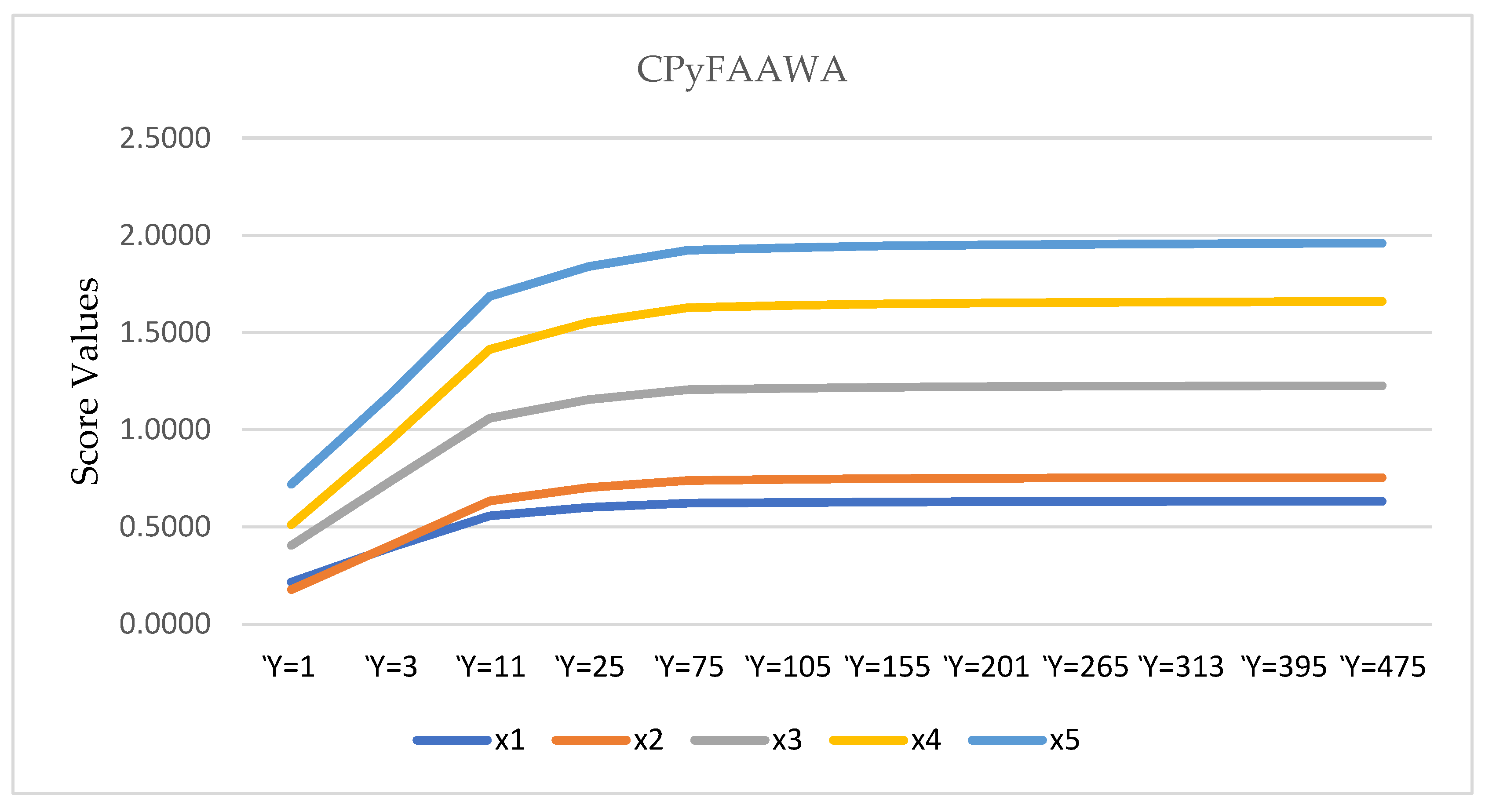
  • Step 5: To analyse suitable applicants, we arranged score values and performed ranking and ordering of the score values in Table 4. We can see that x 1 and x 5 are suitable applicants obtained by CPyFAAWA and CPyFAAWG operators. We also explored obtained score values in the following graphical representation of Figure 2.

7.4. Influence Study

We deploy several parameters   inside the approaches we have mentioned to characterize the alternatives and to demonstrate the influence of various parameter   magnitudes. Table 5 and Table 6 report the ordering consequences of the CPyFAAWA and CPyFAAWG operator-based option selections. It is obvious that as the magnitude   for the CPyFAAWA and CPyFAAWG operators increases; the score values of the alternatives continue rising, but the best option stays the same. This suggests that the provided strategies have the property of isotonicity and that the decision makers can choose the most appropriate value based on their preferences. Furthermore, we see that the results generated by the alternatives seem to be consistent, even when the value varies throughout the demonstration, illustrating the stability of the recommended operators.
We also illustrate the consequences of CPyFAAWA and CPyFAAWG operators as the geometrical representation of Figure 3 and Figure 4, respectively.

8. Comparative Study

To classify the validity and feasibility of our proposed methodologies, we applied several existing AOs to demonstrate information given by the decision makers and displayed in Table 2: the AOs of CPyF-weighted average, (CPyFWA) and CPyF-weighted geometric (CPyFWG) operators by Mahmood et al. [25], AOs of CPyF Dombi-weighted average and CPyF Dombi-weighted operators by Akram et al. [59], AOs of PyF Aczel–Alsina-weighted average (PyFAAWA) and PyF Aczel–Alsina-weighted geometric (PyFAAWG) given by Hussain et al. [58], AOs of interval-valued CPyFWA (IVCPyFWA) and interval-valued CPyFWG (IVCPyFWG) operators by Ali et al. [60], AOs of PyF-weighted average (PyFWA) and PyF-weighted geometric (PyFWG) operators by Rahman et al. [24], and AOs of PyF Einstein-weighted (PyFEW) average (PyFEW) and geometric (PyFEWG) operators by Garg, 2016 [61]. The results of aforementioned existing AOs operators are shown in the following Table 7.
Furthermore, we also illustrate the results of existing AOs as a graphical representation in Figure 5, which is shown above Table 7.

9. Conclusions

Decision-making problems are widespread throughout multiple sectors, including marketing, business and technology. There are a lot of difficulties that decision makers face during the aggregation process due to insufficient information. We used an innovative concept of CPyFSs and developed a list of new AOs based on Aczel–Alsina operations: a CPyFS that has extensive information, including two aspects of MV and NMV in the form of amplitude and phase terms. The main purposes of this article are as follows.
(1)
The main contribution of this article is to present some new AOs and fundamental operational laws of CPyFSs. We generalized the basic idea of Aczel–Alsina TNM and TCNM with operational laws and illustrative examples.
(2)
By using the operational laws of Aczel–Alsina TNM and TCNM, we developed a list of new AOs, like the CPyFAAWA operator, and verified invented AOs with some deserved properties.
(3)
Furthermore, we also established the CPyFAAWAG operator based on the defined fundamental operational laws of Aczel–Alsina TNM and TCNM.
(4)
To find the feasibility and reliability of our invented methodologies, we explored some special cases like CPyFAA-ordered weighted (CPyFAAOW), average (CPyFAAOWA) and CPyFAAOW geometric (CPyFAAOWG) operators, and CPyFAA hybrid-weighted (CPyFAAHW), average (CPyFAAHWA) and CPyFAAHW geometric (CPyFAAHWG) operators with some basic properties.
(5)
By utilizing our invented approaches, we solved an MADM technique. We established an illustrative example to select a suitable candidate for the vacant post of a multinational company.
(6)
To analyze the effectiveness of different parametric values of   on the results of our proposed approaches, we discussed an influence study.
(7)
We checked the reliability and flexibility of our invented approaches by comparing the results of existing AOs with the results of our discussed technique.
The aforementioned operators and approaches will be gradually applied to a range of applications, such as networking analysis, risk assessment, cognitive science, recommender systems, signal processing and many more domains in ambiguous circumstances. Additionally, the interrelationships between the pairs of attributes throughout the aggregation process are not taken into consideration in the current study, but they will be in future ones. To better understand the information in our daily lives, we will also try to establish some more generalized information measurements. We will explore our invented methodologies within the framework of multi-criteria development in the system of the fuzzy environment [62]. We will also explore the concepts of our proposed approaches within the framework of bipolar-valued hesitant fuzzy information [63]. Moreover, we will also explore our current work within the framework of interval type-2 fuzzy systems with quantized output tools [64].

Author Contributions

Conceptualization, H.J., A.H., K.U. and A.J.; Formal analysis, K.U.; Investigation, H.J., A.H., K.U. and A.J.; Software, A.H. and A.J.; Supervision, H.J. and K.U.; Validation, A.H. and A.J.; Visualization, A.H.; Writing—original draft, H.J., A.H., K.U. and A.J.; Writing—review & editing, H.J., A.H., K.U. and A.J. All authors have read and agreed to the published version of the manuscript.

Funding

This research received no external funding.

Institutional Review Board Statement

Not applicable.

Informed Consent Statement

Not applicable.

Data Availability Statement

Not applicable.

Conflicts of Interest

The authors have no conflict of interest regarding this paper.

References

  1. Zadeh, L.A. Fuzzy Sets. Inf. Control 1965, 8, 338–353. [Google Scholar] [CrossRef] [Green Version]
  2. Atanassov, K.T. Intuitionistic Fuzzy Sets. Fuzzy Sets Syst. 1986, 20, 87–96. [Google Scholar] [CrossRef]
  3. Yager, R.R. Pythagorean Fuzzy Subsets. In Proceedings of the 2013 Joint IFSA World Congress and NAFIPS Annual Meeting (IFSA/NAFIPS), Edmonton, AB, Canada, 24–28 June 2013; pp. 57–61. [Google Scholar]
  4. Adlassnig, K.-P. Fuzzy Set Theory in Medical Diagnosis. IEEE Trans. Syst. Man Cybern. 1986, 16, 260–265. [Google Scholar] [CrossRef]
  5. Atanassov, K.T. Interval Valued Intuitionistic Fuzzy Sets. In Intuitionistic Fuzzy Sets; Springer: Berlin/Heidelberg, Germany, 1999; pp. 139–177. [Google Scholar]
  6. Mohd, W.R.W.; Abdullah, L. Similarity Measures of Pythagorean Fuzzy Sets Based on Combination of Cosine Similarity Measure and Euclidean Distance Measure. AIP Conf. Proc. 2018, 1974, 030017. [Google Scholar]
  7. Ramot, D.; Milo, R.; Friedman, M.; Kandel, A. Complex Fuzzy Sets. IEEE Trans. Fuzzy Syst. 2002, 10, 171–186. [Google Scholar] [CrossRef]
  8. Ramot, D.; Friedman, M.; Langholz, G.; Kandel, A. Complex Fuzzy Logic. IEEE Trans. Fuzzy Syst. 2003, 11, 450–461. [Google Scholar] [CrossRef]
  9. Alkouri, A.M.J.S.; Salleh, A.R. Complex Intuitionistic Fuzzy Sets. AIP Conf. Proc. 2012, 1482, 464–470. [Google Scholar]
  10. Ullah, K.; Mahmood, T.; Ali, Z.; Jan, N. On Some Distance Measures of Complex Pythagorean Fuzzy Sets and Their Applications in Pattern Recognition. Complex Intell. Syst. 2020, 6, 15–27. [Google Scholar] [CrossRef] [Green Version]
  11. Riaz, M.; Hashmi, M.R. Linear Diophantine Fuzzy Set and Its Applications towards Multi-Attribute Decision-Making Problems. J. Intell. Fuzzy Syst. 2019, 37, 5417–5439. [Google Scholar] [CrossRef]
  12. Akram, M.; Naz, S. A Novel Decision-Making Approach under Complex Pythagorean Fuzzy Environment. Math. Comput. Appl. 2019, 24, 73. [Google Scholar] [CrossRef] [Green Version]
  13. Khan, R.; Ullah, K.; Pamucar, D.; Bari, M. Performance Measure Using a Multi-Attribute Decision Making Approach Based on Complex T-Spherical Fuzzy Power Aggregation Operators. J. Comput. Cogn. Eng. 2022. [Google Scholar] [CrossRef]
  14. Ali, Z.; Mahmood, T.; Pamucar, D.; Wei, C. Complex Interval-Valued q-Rung Orthopair Fuzzy Hamy Mean Operators and Their Application in Decision-Making Strategy. Symmetry 2022, 14, 592. [Google Scholar] [CrossRef]
  15. Mahmood, T. A Novel Approach towards Bipolar Soft Sets and Their Applications. J. Math. 2020, 2020, 4690808. [Google Scholar] [CrossRef]
  16. Zhang, N.; Su, W.; Zhang, C.; Zeng, S. Evaluation and Selection Model of Community Group Purchase Platform Based on WEPLPA-CPT-EDAS Method. Comput. Ind. Eng. 2022, 172, 108573. [Google Scholar] [CrossRef]
  17. Vojinović, N.; Stević, Ž.; Tanackov, I. A Novel IMF SWARA-FDWGA-PES℡ Analysis for Assessment of Healthcare System. Oper. Res. Eng. Sci. Theory Appl. 2022, 5, 139–151. [Google Scholar] [CrossRef]
  18. Mahmood, T. Multi-Attribute Decision-Making Method Based on Bipolar Complex Fuzzy Maclaurin Symmetric Mean Operators. Comput. Appl. Math. 2022, 41, 331. [Google Scholar] [CrossRef]
  19. Xu, Z. Intuitionistic Fuzzy Aggregation Operators. IEEE Trans. Fuzzy Syst. 2007, 15, 1179–1187. [Google Scholar]
  20. Wei, G. Some Induced Geometric Aggregation Operators with Intuitionistic Fuzzy Information and Their Application to Group Decision Making. Appl. Soft Comput. 2010, 10, 423–431. [Google Scholar] [CrossRef]
  21. Peng, X.; Yuan, H. Fundamental Properties of Pythagorean Fuzzy Aggregation Operators. Fundam. Inform. 2016, 147, 415–446. [Google Scholar] [CrossRef]
  22. Akram, M.; Ullah, K.; Pamucar, D. Performance Evaluation of Solar Energy Cells Using the Interval-Valued T-Spherical Fuzzy Bonferroni Mean Operators. Energies 2022, 15, 292. [Google Scholar] [CrossRef]
  23. Khan, Q.; Mahmood, T.; Ullah, K. Applications of Improved Spherical Fuzzy Dombi Aggregation Operators in Decision Support System. Soft Comput. 2021, 25, 9097–9119. [Google Scholar] [CrossRef]
  24. Rahman, K.; Ali, A.; Shakeel, M.; Khan, M.A.; Ullah, M. Pythagorean Fuzzy Weighted Averaging Aggregation Operator and Its Application to Decision Making Theory. Nucleus 2017, 54, 190–196. [Google Scholar]
  25. Mahmood, T.; Ali, Z.; Ullah, K.; Khan, Q.; AlSalman, H.; Gumaei, A.; Rahman, S.M.M. Complex Pythagorean Fuzzy Aggregation Operators Based on Confidence Levels and Their Applications. Math. Biosci. Eng. 2022, 19, 1078–1107. [Google Scholar] [CrossRef] [PubMed]
  26. Liu, P.; Chen, S.-M.; Wang, Y. Multiattribute Group Decision Making Based on Intuitionistic Fuzzy Partitioned Maclaurin Symmetric Mean Operators. Inf. Sci. 2020, 512, 830–854. [Google Scholar] [CrossRef]
  27. Ullah, K. Picture Fuzzy Maclaurin Symmetric Mean Operators and Their Applications in Solving Multiattribute Decision-Making Problems. Math. Probl. Eng. 2021, 2021, 1098631. [Google Scholar] [CrossRef]
  28. Akram, M.; Dudek, W.A.; Dar, J.M. Pythagorean Dombi Fuzzy Aggregation Operators with Application in Multicriteria Decision-Making. Int. J. Intell. Syst. 2019, 34, 3000–3019. [Google Scholar] [CrossRef]
  29. Chen, T.-Y. A Prioritized Aggregation Operator-Based Approach to Multiple Criteria Decision Making Using Interval-Valued Intuitionistic Fuzzy Sets: A Comparative Perspective. Inf. Sci. 2014, 281, 97–112. [Google Scholar] [CrossRef]
  30. Liu, P.; Wang, P. Multiple-Attribute Decision-Making Based on Archimedean Bonferroni Operators of q-Rung Orthopair Fuzzy Numbers. IEEE Trans. Fuzzy Syst. 2018, 27, 834–848. [Google Scholar] [CrossRef]
  31. Hussain, A.; Ullah, K.; Ahmad, J.; Karamti, H.; Pamucar, D.; Wang, H. Applications of the Multiattribute Decision-Making for the Development of the Tourism Industry Using Complex Intuitionistic Fuzzy Hamy Mean Operators. Comput. Intell. Neurosci. 2022, 2022, 8562390. [Google Scholar] [CrossRef]
  32. Garg, H. Intuitionistic Fuzzy Hamacher Aggregation Operators with Entropy Weight and Their Applications to Multi-Criteria Decision-Making Problems. Iran. J. Sci. Technol. Trans. Electr. Eng. 2019, 43, 597–613. [Google Scholar] [CrossRef]
  33. Akram, M.; Shahzadi, G. A Hybrid Decision-Making Model under q-Rung Orthopair Fuzzy Yager Aggregation Operators. Granul. Comput. 2021, 6, 763–777. [Google Scholar] [CrossRef]
  34. Jan, N.; Zedam, L.; Mahmood, T.; Ullah, K.; Ali, Z. Multiple Attribute Decision Making Method under Linguistic Cubic Information. J. Intell. Fuzzy Syst. 2019, 36, 253–269. [Google Scholar] [CrossRef]
  35. Yang, S.; Pan, Y.; Zeng, S. Decision Making Framework Based Fermatean Fuzzy Integrated Weighted Distance and TOPSIS for Green Low-Carbon Port Evaluation. Eng. Appl. Artif. Intell. 2022, 114, 105048. [Google Scholar] [CrossRef]
  36. Ullah, K.; Mahmood, T.; Jan, N.; Ahmad, Z. Policy Decision Making Based on Some Averaging Aggregation Operators of T-Spherical Fuzzy Sets; a Multi-Attribute Decision Making Approach. Ann. Optim. Theory Pract. 2020, 3, 69–92. [Google Scholar]
  37. Menger, K. Statistical Metrics. Proc. Natl. Acad. Sci. USA 1942, 28, 535. [Google Scholar] [CrossRef]
  38. Klement, E.P. Triangular Norms; Springer: Berlin/Heidelberg, Germany, 2000; Volume 8, ISBN 978-90-481-5507-1. [Google Scholar]
  39. Klement, E.P.; Navara, M. A Characterization of Tribes with Respect to the Łukasiewicz T-Norm. Czechoslov. Math. J. 1997, 47, 689–700. [Google Scholar] [CrossRef] [Green Version]
  40. Wang, S. A Fuzzy Logic for the Revised Drastic Product T-Norm. Soft Comput. 2007, 11, 585–590. [Google Scholar] [CrossRef]
  41. Fodor, J.C. Nilpotent Minimum and Related Connectives for Fuzzy Logic. In Proceedings of the 1995 IEEE International Conference on Fuzzy Systems, Yokohama, Japan, 20–24 March 1995; Volume 4, pp. 2077–2082. [Google Scholar]
  42. Mesiar, R. Nearly Frank T-Norms. Tatra Mt. Math. Publ. 1999, 16, 127–134. [Google Scholar]
  43. Nguyen, H.T.; Kreinovich, V.; Wojciechowski, P. Strict Archimedean T-Norms and t-Conorms as Universal Approximators. Int. J. Approx. Reason. 1998, 18, 239–249. [Google Scholar] [CrossRef] [Green Version]
  44. Wang, W.; Liu, X. Some Operations over Atanassov’s Intuitionistic Fuzzy Sets Based on Einstein t-Norm and t-Conorm. Int. J. Uncertain. Fuzziness Knowl.-Based Syst. 2013, 21, 263–276. [Google Scholar] [CrossRef]
  45. Egbert, R.J. Products and Quotients of Probabilistic Metric Spaces. Pac. J. Math. 1968, 24, 437–455. [Google Scholar] [CrossRef]
  46. Dombi, J. A General Class of Fuzzy Operators, the DeMorgan Class of Fuzzy Operators and Fuzziness Measures Induced by Fuzzy Operators. Fuzzy Sets Syst. 1982, 8, 149–163. [Google Scholar] [CrossRef]
  47. Mahmood, T.; Waqas, H.M.; Ali, Z.; Ullah, K.; Pamucar, D. Frank Aggregation Operators and Analytic Hierarchy Process Based on Interval-Valued Picture Fuzzy Sets and Their Applications. Int. J. Intell. Syst. 2021, 36, 7925–7962. [Google Scholar] [CrossRef]
  48. Liu, P. Some Hamacher Aggregation Operators Based on the Interval-Valued Intuitionistic Fuzzy Numbers and Their Application to Group Decision Making. IEEE Trans. Fuzzy Syst. 2013, 22, 83–97. [Google Scholar] [CrossRef]
  49. Garg, H. Generalized Pythagorean Fuzzy Geometric Aggregation Operators Using Einstein T-Norm and t-Conorm for Multicriteria Decision-Making Process. Int. J. Intell. Syst. 2017, 32, 597–630. [Google Scholar] [CrossRef]
  50. Yan, S.-R.; Guo, W.; Mohammadzadeh, A.; Rathinasamy, S. Optimal Deep Learning Control for Modernized Microgrids. Appl. Intell. 2022. [Google Scholar] [CrossRef]
  51. Mousavi, S.M.; Salimain, S.; Antucheviciene, J. Evaluation of Infrastructure Projects by A Decision Model with Interval-Valued Intuitionistic Fuzzy Sets. Int. J. Strateg. Prop. Manag. 2022, 26, 106–118. [Google Scholar]
  52. Aczél, J.; Alsina, C. Characterizations of Some Classes of Quasilinear Functions with Applications to Triangular Norms and to Synthesizing Judgements. Aequ. Math. 1982, 25, 313–315. [Google Scholar] [CrossRef]
  53. Babu, M.S.; Ahmed, S. Function as the Generator of Parametric T-Norms. Am. J. Appl. Math. 2017, 5, 114–118. [Google Scholar] [CrossRef] [Green Version]
  54. Senapati, T.; Chen, G.; Yager, R.R. Aczel–Alsina Aggregation Operators and Their Application to Intuitionistic Fuzzy Multiple Attribute Decision Making. Int. J. Intell. Syst. 2022, 37, 1529–1551. [Google Scholar] [CrossRef]
  55. Senapati, T.; Chen, G.; Mesiar, R.; Yager, R.R. Novel Aczel–Alsina Operations-Based Interval-Valued Intuitionistic Fuzzy Aggregation Operators and Their Applications in Multiple Attribute Decision-Making Process. Int. J. Intell. Syst. 2021, 38, 5059–5081. [Google Scholar] [CrossRef]
  56. Naeem, M.; Khan, Y.; Ashraf, S.; Weera, W.; Batool, B. A Novel Picture Fuzzy Aczel-Alsina Geometric Aggregation Information: Application to Determining the Factors Affecting Mango Crops. AIMS Math. 2022, 7, 12264–12288. [Google Scholar] [CrossRef]
  57. Hussain, A.; Ullah, K.; Yang, M.-S.; Pamucar, D. Aczel-Alsina Aggregation Operators on T-Spherical Fuzzy (TSF) Information with Application to TSF Multi-Attribute Decision Making. IEEE Access 2022, 10, 26011–26023. [Google Scholar] [CrossRef]
  58. Hussain, A.; Ullah, K.; Alshahrani, M.N.; Yang, M.-S.; Pamucar, D. Novel Aczel–Alsina Operators for Pythagorean Fuzzy Sets with Application in Multi-Attribute Decision Making. Symmetry 2022, 14, 940. [Google Scholar] [CrossRef]
  59. Akram, M.; Khan, A.; Borumand Saeid, A. Complex Pythagorean Dombi Fuzzy Operators Using Aggregation Operators and Their Decision-Making. Expert Syst. 2021, 38, e12626. [Google Scholar] [CrossRef]
  60. Ali, Z.; Mahmood, T.; Ullah, K.; Khan, Q. Einstein Geometric Aggregation Operators Using a Novel Complex Interval-Valued Pythagorean Fuzzy Setting with Application in Green Supplier Chain Management. Rep. Mech. Eng. 2021, 2, 105–134. [Google Scholar] [CrossRef]
  61. Garg, H. A New Generalized Pythagorean Fuzzy Information Aggregation Using Einstein Operations and Its Application to Decision Making. Int. J. Intell. Syst. 2016, 31, 886–920. [Google Scholar] [CrossRef]
  62. Zeng, S.; Hu, Y.; Llopis-Albert, C. Stakeholder-Inclusive Multi-Criteria Development of Smart Cities. J. Bus. Res. 2023, 154, 113281. [Google Scholar] [CrossRef]
  63. Khan, M.U.; Mahmood, T.; Ullah, K.; Jan, N.; Deli, I. Some Aggregation Operators for Bipolar-Valued Hesitant Fuzzy Information Based on Einstein Operational Laws. J. Eng. Appl. Sci. JEAS 2017, 36, 63–72. [Google Scholar]
  64. Sakthivel, R.; Kavikumar, R.; Mohammadzadeh, A.; Kwon, O.-M.; Kaviarasan, B. Fault Estimation for Mode-Dependent IT2 Fuzzy Systems with Quantized Output Signals. IEEE Trans. Fuzzy Syst. 2020, 29, 298–309. [Google Scholar] [CrossRef]
Figure 1. Flow chart of this article.
Symmetry 15 00068 g001
Figure 2. The score values of the CPyFAAWA and CPyFAAWG operators.
Symmetry 15 00068 g002
Figure 3. The results of CPyFAAWA operators for   .
Symmetry 15 00068 g003
Figure 4. The results of CPyFAAWG operators for Ὺ.
Symmetry 15 00068 g004
Figure 5. The results of the comparative analysis.
Symmetry 15 00068 g005
Table 1. Symbols and their meanings.
SymbolMeaningSymbolMeaning
Non-empty set R ˘ Score function
Π MV of amplitude term A ˘ Accuracy function
α MV of phase term Ω CPyFV
Ξ NMV of amplitude term D Weight vector
β NMV of phase term Ŧ TNM
ψ Alternative TCNM
ʊ Attribute Decision matrix
Table 2. Decision matrix using the information of the CPyFVs.
J 1 J 2
x 1 0.55 e 2 i π 0.29 ,   0.46 e 2 i π 0.71 0.46 e 2 i π 0.67 ,   0.45 e 2 i π 0.09
x 2 0.46 e 2 i π 0.33 ,   0.09 e 2 i π 0.41 0.17 e 2 i π 0.27 ,   0.45 e 2 i π 0.61
x 3 0.45 e 2 i π 0.61 ,   0.88 e 2 i π 0.28 0.67 e 2 i π 0.45 ,   0.62 e 2 i π 0.45
x 4 0.36 e 2 i π 0.71 ,   0.46 e 2 i π 0.67 0.36 e 2 i π 0.68 ,   0.36 e 2 i π 0.56
x 5 0.48 e 2 i π 0.67 ,   0.19 e 2 i π 0.37 0.56 e 2 i π 0.67 ,   0.19 e 2 i π 0.37
J 3 J 4
x 1 082 e 2 i π 0.27 ,   0.43 e 2 i π 0.61 0.56 e 2 i π 0.81 ,   0.23 e 2 i π 0.09
x 2 0.39 e 2 i π 0.36 ,   0.35 e 2 i π 0.55 0.19 e 2 i π 0.46 ,   0.53 e 2 i π 0.47
x 3 0.55 e 2 i π 0.78 ,   0.18 e 2 i π 0.28 0.49 e 2 i π 0.47 ,   0.29 e 2 i π 0.38
x 4 0.47 e 2 i π 0.58 ,   0.42 e 2 i π 0.38 0.8 e 2 i π 0.48 ,   0.53 e 2 i π 0.45
x 5 0.57 e 2 i π 0.61 ,   0.38 e 2 i π 0.63 0.47 e 2 i π 0.57 ,   0.47 e 2 i π 0.48
Table 3. Consequences of CPyFAAWA and CPyFAAWG operators.
CPyFAAWA CPyFAAWG
0.7416 e 2 i π 0.6545 ,   0.3959 e 2 i π 0.1821 0.5554 e 2 i π 0.3292 ,   0.4398 e 2 i π 0.6357
04035 e 2 i π 0.3635 ,   0.1863 e 2 i π 0.4908 0.2681 e 2 i π 0.3276 ,   0.4196 e 2 i π 0.5471
0.5864 e 2 i π 0.7046 ,   0.2847 e 2 i π 0.3137 0.5199 e 2 i π 0.5509 ,   0.7965 e 2 i π 0.3774
0.6195 e 2 i π 0.6609 ,   0.4185 e 2 i π 0.4685 0.4050 e 2 i π 0.6086 ,   0.4456 e 2 i π 0.5909
0.5409 e 2 i π 0.6461 ,   0.2411 e 2 i π 0.4273 0.5229 e 2 i π 0.6333 ,   0.3648 e 2 i π 0.5533
Table 4. Ranking and ordering of the score values.
Operators S x 1 S x 2 S x 3 S x 4 S x 5 Ranking and Ordering
CPyFAAWA 0.3942 0.0097 0.3304 0.2130 0.2347 x 1 x 3 x 5 x 4 x 2
CPyFAAWG 0.0904 0.1481 0.1015 0.0067 0.1176 x 5 x 4 x 1 x 3 x 2
Table 5. The ordering and ranking of the obtained consequences of CPyFAAWA operators.
S x 1 S x 2 S x 3 S x 4 S x 5 Ordering and Ranking
= 1 0.2169 0.0383 0.2275 0.1062 0.2082 x 3 x 1 x 5 x 4 x 2
= 3 0.3942 0.0097 0.3304 0.2130 0.2347 x 1 x 3 x 5 x 4 x 2
= 11 0.5562 0.0771 0.4259 0.3534 0.2733 x 1 x 3 x 4 x 5 x 2
= 25 0.6004 0.1024 0.4524 0.3967 0.2874 x 1 x 3 x 4 x 5 x 2
= 75 0.6228 0.1164 0.4663 0.4222 0.2957 x 1 x 3 x 4 x 5 x 2
= 105 0.6260 0.1184 0.4683 0.4259 0.2970 x 1 x 3 x 4 x 5 x 2
= 155 0.6285 0.1201 0.4699 0.4288 0.2981 x 1 x 3 x 4 x 5 x 2
= 201 0.6297 0.1209 0.4707 0.4303 0.2986 x 1 x 3 x 4 x 5 x 2
= 265 0.6307 0.1215 0.4713 0.4314 0.2991 x 1 x 3 x 4 x 5 x 2
= 313 0.6311 0.1218 0.4716 0.4320 0.2993 x 1 x 3 x 4 x 5 x 2
= 395 0.6317 0.1222 0.4719 0.4326 0.2995 x 1 x 3 x 4 x 5 x 2
= 475 0.6320 0.1224 0.4722 0.4330 0.2997 x 1 x 3 x 4 x 5 x 2
Table 6. The ordering and ranking of the obtained consequences of CPyFAAWG operators.
S x 1 S x 2 S x 3 S x 4 S x 5 Ordering and Ranking
= 1 0.0089 0.0982 0.0436 0.0485 0.1721 x 5 x 4 x 3 x 1 x 2
= 3 0.0904 0.1481 0.1015 0.0067 0.1176 x 5 x 4 x 1 x 3 x 2
= 11 0.1653 0.2190 0.2223 0.1033 0.0403 x 5 x 4 x 1 x 2 x 2
= 25 0.1911 0.2487 0.2566 0.1474 0.0043 x 5 x 4 x 1 x 2 x 3
= 75 0.2070 0.2666 0.2760 0.1724 0.0208 x 5 x 4 x 1 x 2 x 3
= 105 0.2094 0.2691 0.2788 0.1760 0.0249 x 5 x 4 x 1 x 2 x 3
= 155 0.2114 0.2712 0.2811 0.1788 0.0284 x 5 x 4 x 1 x 2 x 3
= 201 0.2124 0.2722 0.2822 0.1802 0.0301 x 5 x 4 x 1 x 2 x 3
= 265 0.2131 0.2730 0.2831 0.1814 0.0315 x 5 x 4 x 1 x 2 x 3
= 313 0.2135 0.2734 0.2836 0.1819 0.0322 x 5 x 4 x 1 x 2 x 3
= 395 0.2140 0.2739 0.2841 0.1825 0.0330 x 5 x 4 x 1 x 2 x 3
= 475 0.2142 0.2742 0.2844 0.1829 0.0335 x 5 x 4 x 1 x 2 x 3
Table 7. The results of existing AOs and our proposed methodologies.
Aggregation Operators Environment Ranking and Ordering
CPyFAAWACPyFVs x 1 x 3 x 5 x 4 x 2
CPyFAAWGCPyFVs x 5 x 4 x 1 x 3 x 2
CPyFWA [25]CPyFVs x 3 x 1 x 5 x 4 x 2
CPyFWG [25]CPyFVs x 5 x 4 x 3 x 1 x 2
CPyFDWAA [59]CPyFVs x 1 x 3 x 5 x 4 x 2
CPyFDWGA [59]CPyFVs x 5 x 4 x 3 x 1 x 2
PFAAWA/PFAAWG [58]PyFVsFailed
IVCPyFWA/IVCPyFWA [60]IVCPyFVsFailed
PyFWA/PyFWG [24]PyFVsFailed
PyFEWA/PyFEWG [61]PyFVsFailed
Disclaimer/Publisher’s Note: The statements, opinions and data contained in all publications are solely those of the individual author(s) and contributor(s) and not of MDPI and/or the editor(s). MDPI and/or the editor(s) disclaim responsibility for any injury to people or property resulting from any ideas, methods, instructions or products referred to in the content.

