General Entropy with Bayes Techniques under Lindley and MCMC for Estimating the New Weibull–Pareto Parameters: Theory and Application

Abstract

Censored data play a pivotal role in life testing experiments since they significantly reduce cost and testing time. Hence, this paper investigates the problem of statistical inference for a system of progressive first-failure censoring data for a new Weibull–Pareto distribution. Maximum likelihood estimates for the parameters as well as some lifetime indices such as reliability, hazard rate functions, and coefficient of variation are derived. Lindley approximation and the Markov chain Monte Carlo technique are applied to obtain the Bayes estimates relative to two different loss functions: balanced linear exponential and general entropy loss functions. The results of the Bayes estimate are computed under the consideration of informative prior function. A real-life example "the survival times in years of a group of patients given chemotherapy treatment" is presented to illustrate the proposed methods. Finally, a simulation study is carried out to determine the performance of the maximum likelihood and Bayes estimates and compare the performance of different corresponding confidence intervals.

1. Introduction

In life testing experiments, one of the major reasons for the removal of experimental units is saving the working experimental units for future use, saving the cost and time associated with testing. This leads us to the use of censoring schemes. The most common schemes are considered Type-I and Type-II censoring. These types have been studied by several statisticians; see, for instance, Kundu and Howlader [1] and Fujii [2]. In terms of the procedure, in Type-I censoring, all units n are put in the test for a pre-specified time and at the end of the specified time, the test ends. In Type-II censoring, all units n are put in the test, and the test is terminated at the failure of the pre-specified m-th unit $(1\le m\le n)$. The disadvantages of these types are represented in that the units cannot be removed during the test. Thus, progressive Type-II censoring (PT2C) was proposed, which has more flexibility in allowing units to be withdrawn within the duration of the test.

An excellent reference that accurately describes this type of censoring scheme is Balakrishnan and Sandhu [3], who add to the steps of generation, which is useful to achieve the desired goals of using censoring schemes. Several authors have discussed inference under PT2C with applications, see, for example, Chen et al. [4], Xu et al. [5], Luo et al. [6], and EL-Sagheer [7].

Although the experimental efficiency under PT2C can be significantly improved, the duration of the test is still too long. So, Johnson [8] described a life test in which the experimenter can be decided to divide the units under test into several groups and then run all the units simultaneously until the occurrence of the first failure in each group. Such a censoring scheme is called first-failure censoring (FFC). However, using this censoring scheme does not enable the experimenter to remove experimental units from the test until the first failure is observed. For this reason, Wu and Kuş [9] introduced life testing, which combined FFC with PT2C, and is named the progressive first-failure censoring (Pro-F-F-C) scheme. Many authors have discussed inference under a Pro-F-F-C scheme for different lifetime distributions, see, for example, Soliman et al. [10], Soliman et al. [11,12], Soliman et al. [13], Mahmoud et al. [14,15], Abushal [16], Ahemd [17], Xie and Gui [18], Shi and Shi [19], and EL-Sagheer et al. [20].

A new Weibull–Pareto distribution (NWPD) is a generalization of the Weibull and Pareto distributions, as discussed in Suleman and Albert [21]. The probability density function (pdf) and cumulative distribution function (cdf) of a random variable X has an NWPD given, respectively, by

$$f\left(x;\delta ,\beta ,\theta \right)=\frac{\beta \delta }{\theta }{\left(\frac{x}{\theta }\right)}^{\beta -1}{e}^{-\delta {\left(\frac{x}{\theta }\right)}^{\beta }},x>0;\delta ,\beta ,\theta >0,$$

(1)

and

$$F\left(x;\delta ,\beta ,\theta \right)=1-e^{-\delta {\left(\frac{x}{\theta }\right)}^{\beta }},$$

(2)

where $\delta$ and $\theta$ are the scale parametersand $\beta$ is the shape parameter. The reliability function $S\left(t\right)$, hazard rate function $h\left(t\right)$, and coefficient of variation $CV$ of the NWPD ($\delta ,\beta ,\theta$) are, respectively, given by

$$S\left(t\right)=e^{-\delta {\left(\frac{t}{\theta }\right)}^{\beta }},t>0,$$

(3)

$$h\left(t\right)=\frac{\beta \delta }{\theta }{\left(\frac{t}{\theta }\right)}^{\beta -1},t>0,$$

(4)

and

$$CV=\frac{\sqrt{\mathsf{\Gamma }\left(\frac{\beta +2}{\beta }\right)-{\left[\mathsf{\Gamma }\left(\frac{\beta +1}{\beta }\right)\right]}^2}}{\mathsf{\Gamma }\left(\frac{\beta +1}{\beta }\right)},\beta >0.$$

(5)

The importance of studying this model is due to the fact that it is an interesting three-parameter lifetime model, and it can be a useful characterization of the survival time of a given system because of its analytical structure. In addition, it occupies an important position in reliability analysis, biomedical, and life-test experiences. From $h\left(t\right)$, the following can be observed: If $\beta =1,$ the $h\left(t\right)$ is constant and given by $h\left(t\right)=\frac{\delta }{\theta }$, this makes the NWPD suitable for modeling systems or components with constant failure rate. If $\beta >1$, the hazard rate function is an increasing function of x, which makes the NWPD suitable for modeling components that wear faster with time. If $\beta <1$, the hazard rate function is a decreasing function of x, which makes the NWPD suitable for modeling components that wear slower with time. For more details about the NWPD, including its properties and applications see Suleman and Albert [21]. Several authors have discussed the statistical inference of censored data on the NWPD, for example, Almetwally et al. [22], Al-Omari et al. [23], EL-Sagheer et al. [24], and Mahmoud et al. [25].

This article aims to discuss the statistical inference of the NWPD parameters as well as some lifetime indices such as reliability function, hazard rate function, and coefficient of variation in the presence of Pro-F-F-C scheme. To this end, both point and interval estimations are discussed by implementing classical and Bayesian approaches. Moreover, delta, log transformation ($\mathcal{L}$T) and arc sine transformation (AST) methods are used to construct the ACIs for $S\left(t\right)$, $h\left(t\right)$, and $CV$. In the Bayesian framework, Lindley and MCMC techniques under two different loss functions (balanced linear exponential (BLINEX) and general entropy (GE)) are proposed. A simulation study is carried out to determine the performance of the ML, Lindley, and MCMC estimation and compare the performance of different corresponding confidence intervals. Finally, the application to real-life data on gastric cancer survival times is analyzed for illustrative purposes.

The rest of this article is organized as follows: MLEs for the unknown quantities are presented in Section 2. In Section 3, the ACIs are constructed. Bayes estimators relative to different loss functions are also considered in Section 4. Section 5 provided the illustration of the proposed procedure by using a real-life example. Simulation results are discussed in Section 6. Finally, concluding remarks are investigated in Section 7.

2. ML Inference

Suppose that $x_{i:m:n:k}^R$, $i=1,2,\dots ,m$, is a Pro-F-F-C order statistic from NWPD with the scheme $R=\left(R_1,R_2,\dots ,R_m\right)$. According to Wu and Kuş [9], the joint pdf can be written as

$$L(\underline{x};\delta ,\beta ,\theta )\propto k^m{\beta }^m{\delta }^m{\theta }^{(-m)}\left[\prod _{i=1}^m{\left(\frac{x_i}{\theta }\right)}^{\beta -1}\right]exp\left\{-\delta \sum _{i=1}^{m}k\left(R_i+1\right){\left(\frac{x_i}{\theta }\right)}^{\beta }\right\}.$$

(6)

The log-likelihood function $\ell \left(\underline{x};\delta ,\beta ,\theta \right)$ can be written as

$$\begin{array}{c}\hfill \begin{array}{cc}\hfill \ell (\underline{x};\delta ,\beta ,\theta )=& mln\left(k\right)+mln\left(\beta \right)+mln\left(\delta \right)-mln\left(\theta \right)+(\beta -1)\sum _{i=1}^{m}ln\left(\frac{x_i}{\theta }\right)\hfill \\ & -\delta \sum _{i=1}^{m}k\left(R_i+1\right){\left(\frac{x_i}{\theta }\right)}^{\beta }.\hfill \end{array}\end{array}$$

(7)

By setting the partial derivatives of Equation (7) with respect to $\delta$, $\beta$, and $\theta$ to zero, the MLEs can be obtained by soluting the following likelihood equations

$$\frac{m}{\delta }-\sum _{i=1}^{m}k\left(R_i+1\right){\left(\frac{x_i}{\theta }\right)}^{\beta }=0,$$

(8)

$$\frac{m}{\beta }+\sum _{i=1}^{m}ln\left(\frac{x_i}{\theta }\right)-\delta \sum _{i=1}^{m}k\left(R_i+1\right){\left(\frac{x_i}{\theta }\right)}^{\beta }ln\left(\frac{x_i}{\theta }\right)=0,$$

(9)

and

$$\frac{m\beta }{\theta }-\frac{\beta \delta }{\theta }\sum _{i=1}^{m}k\left(R_i+1\right){\left(\frac{x_i}{\theta }\right)}^{\beta }=0.$$

(10)

Since the non-linear Equations (8)–(10) cannot be solved analytically, a numerical method such as the Newton–Raphson method is used. Thus, we can be computed the MLEs of $S\left(t\right)$, $h\left(t\right)$, and $CV$ by using the invariant property of the MLEs.

3. Constructing the ACIs

In this section, the ML estimate, delta, $\mathcal{L}$T, and AST methods are discussed to explain how to originate the CIs of unknown quantities.

3.1. The ML Estimate

Based on the invariant property of the MLEs, the ACIs of the parameters can be constructed via asymptotic variances that can be acquired from the inverse of the Fisher information matrix (IFIM). Therefore, the IFIM can be determined according to the likelihood equations through the following expression

$${\widehat{I}}_{ij}^{-1}\left(\mathsf{\Phi }\right)={\left[E\left(\frac{-{\partial }^2\ell \left(\mathsf{\Phi }\right)}{\partial {\varphi }_i\partial {\varphi }_j}\right)\right]}^{-1},i,j=1,2,3,\mathsf{\Phi }=\left({\varphi }_1,{\varphi }_2,{\varphi }_3\right)=\left(\delta ,\beta ,\theta \right),$$

(11)

where

$${\ell }_{\delta \delta }=\frac{-m}{{\delta }^2},{\ell }_{\delta \beta }=-\sum _{i=1}^{m}k\left(R_i+1\right){\left(\frac{x_i}{\theta }\right)}^{\beta }ln\left(\frac{x_i}{\theta }\right)={\ell }_{\beta \delta },$$

(12)

$${\ell }_{\delta \theta }=\frac{\beta }{\theta }\sum _{i=1}^{m}k\left(R_i+1\right){\left(\frac{x_i}{\theta }\right)}^{\beta }={\ell }_{\theta \delta },$$

(13)

$${\ell }_{\beta \beta }=\frac{-m}{{\beta }^2}-\delta \sum _{i=1}^{m}k\left(R_i+1\right){\left(\frac{x_i}{\theta }\right)}^{\beta }{\left(ln\left(\frac{x_i}{\theta }\right)\right)}^2,$$

(14)

$${\ell }_{\beta \theta }=\frac{-m}{\theta }+\frac{\delta \beta }{\theta }\sum _{i=1}^{m}k\left(R_i+1\right){\left(\frac{x_i}{\theta }\right)}^{\beta }ln\left(\frac{x_i}{\theta }\right)+\frac{\delta }{\theta }\sum _{i=1}^{m}k\left(R_i+1\right){\left(\frac{x_i}{\theta }\right)}^{\beta }={\ell }_{\theta \beta },$$

(15)

and

$${\ell }_{\theta \theta }=\frac{m\beta }{{\theta }^2}-\frac{\beta (\beta +1)\delta }{{\theta }^2}\sum _{i=1}^{m}k\left(R_i+1\right){\left(\frac{x_i}{\theta }\right)}^{\beta }.$$

(16)

Due to the difficulty of calculating the exact expression of Equation (11), the asymptotic variance–covariance matrix will be used as the follows

$${\widehat{I}}^{-1}\left(\delta ,\beta ,\theta \right)=\left(\begin{array}{ccc}Var\left(\widehat{\delta }\right)& Cov\left(\widehat{\delta },\widehat{\beta }\right)& Cov\left(\widehat{\delta },\widehat{\theta }\right)\\ Cov\left(\widehat{\beta },\widehat{\delta }\right)& Var\left(\widehat{\beta }\right)& Cov\left(\widehat{\beta },\widehat{\theta }\right)\\ Cov\left(\widehat{\theta },\widehat{\delta }\right)& Cov\left(\widehat{\theta },\widehat{\beta }\right)& Var\left(\widehat{\theta }\right)\end{array}\right).$$

(17)

Hence, $\left(\widehat{\delta },\widehat{\beta },\widehat{\theta }\right)\sim N\left[\left(\delta ,\beta ,\theta \right),{\widehat{I}}^{-1}\left(\delta ,\beta ,\theta \right)\right]$, and then the $\left(1-\gamma \right)100\%$ ACIs for $\mathsf{\Phi }=$$\left(\delta ,\beta ,\theta \right)$ are given by

$$\left[\widehat{\mathsf{\Phi }}-Z_{\gamma /2}\sqrt{Var\left(\widehat{\mathsf{\Phi }}\right)},\widehat{\mathsf{\Phi }}+Z_{\gamma /2}\sqrt{Var\left(\widehat{\mathsf{\Phi }}\right)}\right],$$

(18)

where $Z_{\gamma /2}$ is the standard normal distribution percentile with probability right-tailed $\gamma /2$.

3.2. Delta Method

The $\left(1-\gamma \right)100\%$ ACIs for $\mathsf{\Psi }=\left(S\left(t\right),h\left(t\right),CV\right)$ can be given by

$$\left[\widehat{\mathsf{\Psi }}-Z_{\gamma /2}\sqrt{Var\left(\widehat{\mathsf{\Psi }}\right)},\widehat{\mathsf{\Psi }}+Z_{\gamma /2}\sqrt{Var\left(\widehat{\mathsf{\Psi }}\right)}\right],$$

(19)

where $Var\left(\widehat{\mathsf{\Psi }}\right)$ is the variance of $\widehat{\mathsf{\Psi }}$, which can be obtained by using the delta method, see Green [26], and can be written as

$$Var\left(\widehat{\mathsf{\Psi }}\right)\simeq {\left[B^T{\widehat{I}}^{-1}B\right]}_{\left(\widehat{\delta },\widehat{\beta },\widehat{\theta }\right)},$$

(20)

where B is the first derivative of $\widehat{\mathsf{\Psi }}$ with respect to $\widehat{\delta },$$\widehat{\beta }$, and $\widehat{\theta }$, $B_i^T$ is the transpose matrix of B and ${\widehat{I}}^{-1}$ is in (17).

3.3. Log Transformation Method

The $\left(1-\gamma \right)100\%$$\mathcal{L}$TCIs for $\mathsf{\Psi }=\left(S\left(t\right),h\left(t\right),CV\right)$ can be obtained, respectively, by

$$ln\left(\frac{\widehat{\mathsf{\Psi }}}{1-\widehat{\mathsf{\Psi }}}\right)\mp Z_{\gamma /2}\frac{\sqrt{Var\left(\widehat{\mathsf{\Psi }}\right)}}{1-\widehat{\mathsf{\Psi }}}.$$

(21)

If $(L,U)$ denote the lower and upper bounds of $\mathcal{L}$TCIs of $\mathsf{\Psi }$, then the $\left(1-\gamma \right)100\%$ ACIs for $\mathsf{\Psi }$ relative to $\mathcal{L}$T are given by

$$\left[e^L{\left(1+e^L\right)}^{-1},e^U{\left(1+e^U\right)}^{-1}\right].$$

(22)

3.4. Arcsin Transformation Method

The $\left(1-\gamma \right)100\%$ ASTCIs for $\mathsf{\Psi }=\left(S\left(t\right),h\left(t\right),CV\right)$ can be obtained by

$$arcsin\left(\sqrt{\widehat{\mathsf{\Psi }}}\right)\mp Z_{\gamma /2}\sqrt{\frac{Var\left(\widehat{\mathsf{\Psi }}\right)}{4\widehat{\mathsf{\Psi }}\left(1-\widehat{\mathsf{\Psi }}\right)}}.$$

(23)

If $(L,U)$ denote the lower and upper bounds of ASTCIs of $\mathsf{\Psi }$, then the $\left(1-\gamma \right)100\%$ ACIs for $\mathsf{\Psi }$ relative to AST are given by

$$\left[{sin}^2\left(L\right),{sin}^2\left(U\right)\right].$$

(24)

For more details about $\mathcal{L}$T and AST, see Mukherjee and Maiti [27], Krishnamoorthy and Lin [28], and Ahmed [29].

4. Bayesian Estimation

In this section, we discuss how to obtain the Bayes estimates and construct the corresponding CRIs for $\delta$, $\beta$, and $\theta$, $S\left(t\right)$, $h\left(t\right)$, and $CV$ under BLINEX and GE loss functions. Therefore, we consider that the unknown parameters $\delta$, $\beta$, and $\theta$ are stochastically independently distributed with conjugate gamma prior. Hence, the joint prior density can be formulated as follows

$$\pi \left(\delta ,\beta ,\theta \right)\propto {\delta }^{{\gamma }_1-1}{\beta }^{{\gamma }_2-1}{\theta }^{{\gamma }_3-1}exp\left\{-{\eta }_1\delta -{\eta }_2\beta -{\eta }_3\theta \right\},$$

(25)

where the hyperparameters ${\gamma }_i$ and ${\eta }_i$ (where $i=1,2,3$) are reflected prior knowledge about $\delta$, $\beta$, and $\theta$. Consequently, from (6) and (25), the joint posterior density can be expressed as follows

$$\begin{array}{c}\hfill \begin{array}{cc}\hfill {\pi }^{*}(\delta ,\beta ,\theta \mid \underline{x})=& \frac{L(\underline{x};\delta ,\beta ,\theta )\times \pi (\delta ,\beta ,\theta )}{{\int }_0^{\infty }{\int }_0^{\infty }{\int }_0^{\infty }L(\underline{x};\delta ,\beta ,\theta )\times \pi (\delta ,\beta ,\theta )d\delta d\beta d\theta }\hfill \\ \hfill \propto & {\beta }^{m+{\gamma }_2-1}{\delta }^{m+{\gamma }_1-1}{\theta }^{\left(-m+{\gamma }_3-1\right)}\left[\prod _{i=1}^m{\left(\frac{x_i}{\theta }\right)}^{\beta -1}\right]\hfill \\ & \times exp\left\{-{\eta }_2\beta -{\eta }_3\theta -\delta \left[{\eta }_1+\sum _{i=1}^{m}k\left(R_i+1\right){\left(\frac{x_i}{\theta }\right)}^{\beta }\right]\right\}.\hfill \end{array}\end{array}$$

(26)

The Bayes estimate of the unknown quantity $q\left(\delta ,\beta ,\theta \right)$ under BLINEX and GE loss functions is given by

$$\left.\begin{array}{c}{\widehat{q}}_{BL}\left(\delta ,\beta ,\theta \right)=\frac{-1}{c}log\left(\omega e^{-cq\left(\delta ,\beta ,\theta \right)}+\left(1+\omega \right)E\left[e^{-cq\left(\delta ,\beta ,\theta \right)}|\underline{x}\right]\right)\\ {\widehat{q}}_{GE}\left(\delta ,\beta ,\theta \right)={\left(E\left[{\left(q\left(\delta ,\beta ,\theta \right)\right)}^{-b}|\underline{x}\right]\right)}^{\frac{-1}{b}}\end{array}\right\},$$

(27)

where the posterior expectations of $q\left(\delta ,\beta ,\theta \right)$ under BLINEX and GE loss functions can be written as

$$\left.\begin{array}{c}E\left[e^{-cq\left(\delta ,\beta ,\theta \right)}|\underline{x}\right]=\frac{{\int }_0^{\infty }{\int }_0^{\infty }{\int }_0^{\infty }{e}^{-cq\left(\delta ,\beta ,\theta \right)}\times L(\underline{x};\delta ,\beta ,\theta )\times \pi \left(\delta ,\beta ,\theta \right)d\delta d\beta d\theta }{{\int }_0^{\infty }{\int }_0^{\infty }{\int }_0^{\infty }L(\underline{x};\delta ,\beta ,\theta )\times \pi \left(\delta ,\beta ,\theta \right)d\delta d\beta d\theta }\\ E\left[{\left(q\left(\delta ,\beta ,\theta \right)\right)}^{-b}|\underline{x}\right]=\frac{{\int }_0^{\infty }{\int }_0^{\infty }{\int }_0^{\infty }{\left(q\left(\delta ,\beta ,\theta \right)\right)}^{-b}\times L(\underline{x};\delta ,\beta ,\theta )\times \pi \left(\delta ,\beta ,\theta \right)d\delta d\beta d\theta }{{\int }_0^{\infty }{\int }_0^{\infty }{\int }_0^{\infty }L(\underline{x};\delta ,\beta ,\theta )\times \pi \left(\delta ,\beta ,\theta \right)d\delta d\beta d\theta }\end{array}\right\}.$$

(28)

It is noticeable that the Bayes estimates in both kinds of loss functions include three integrals and cannot be constructed in closed forms. Therefore, the Lindley and MCMC techniques will be implemented to obtain the Bayes estimates of the unknown quantities.

4.1. Lindley’s Approximation

There are various methods suggested to approximate the ratio of integrals of the above form, maybe the simplest one is the Lindley [30] approximation method, which approximates the Bayes estimates into a form containing no integrals. Many authors have used this approximation, see for example, Sarhan et al. [31], Sultan et al. [32], Singh et al. [33], Singh et al. [34], and Rastogi and Tripathi [35]. In short, this method works as follows: for any ratio of the integral of the form

$$I\left(x\right)=E[u(\delta ,\beta ,\theta )\mid \underline{x}]=\frac{\underset{(\delta ,\beta ,\theta )}{\int }u(\delta ,\beta ,\theta )e^{\ell (\delta ,\beta ,\theta )+\rho (\delta ,\beta ,\theta )}d(\delta ,\beta ,\theta )}{\underset{(\delta ,\beta ,\theta )}{\int }{e}^{\ell (\delta ,\beta ,\theta )+\rho (\delta ,\beta ,\theta )}d(\delta ,\beta ,\theta )},$$

(29)

where $u\left(\delta ,\beta ,\theta \right)$ is the function of $\delta$, $\beta$, and $\theta$ only, $\rho \left(\delta ,\beta ,\theta \right)=log\pi \left(\delta ,\beta ,\theta \right)$, and $\pi \left(\delta ,\beta ,\theta \right)$ is the joint prior density. Hence, $I\left(x\right)$ can be estimated as

$$\begin{array}{ccc}\hfill I\left(x\right)& =& u\left(\widehat{\delta },\widehat{\beta },\widehat{\theta }\right)+\left({\widehat{u}}_{\delta }{a}_1+{\widehat{u}}_{\beta }{a}_2+{\widehat{u}}_{\theta }{a}_3+a_4+a_5\right)+\frac{1}{2}\left[A\left({\widehat{u}}_{\delta }{\widehat{\sigma }}_{\delta \delta }+{\widehat{u}}_{\beta }{\widehat{\sigma }}_{\delta \beta }+{\widehat{u}}_{\theta }{\widehat{\sigma }}_{\delta \theta }\right)\right.\hfill \\ & & \left.+B\left({\widehat{u}}_{\delta }{\widehat{\sigma }}_{\beta \delta }+{\widehat{u}}_{\beta }{\widehat{\sigma }}_{\beta \beta }+{\widehat{u}}_{\theta }{\widehat{\sigma }}_{\beta \theta }\right)+C\left({\widehat{u}}_{\delta }{\widehat{\sigma }}_{\theta \delta }+{\widehat{u}}_{\beta }{\widehat{\sigma }}_{\theta \beta }+{\widehat{u}}_{\theta }{\widehat{\sigma }}_{\theta \theta }\right)\right],\hfill \end{array}$$

(30)

where $\widehat{\delta }$, $\widehat{\beta }$, and $\widehat{\theta }$ are the MLEs of $\delta$, $\beta$, and $\theta$, respectively, and subscripts 1, 2, and 3 on the right-hand sides refer to $\delta$, $\beta$, and $\theta$.

$$\left.\begin{array}{c}{a}_i={\widehat{\rho }}_{\delta }{\widehat{\sigma }}_{i\delta }+{\widehat{\rho }}_{\beta }{\widehat{\sigma }}_{i\beta }+{\widehat{\rho }}_{\theta }{\widehat{\sigma }}_{i\theta }\\ a_4={\widehat{u}}_{\delta \beta }{\widehat{\sigma }}_{\delta \beta }+{\widehat{u}}_{\delta \theta }{\widehat{\sigma }}_{\delta \theta }+{\widehat{u}}_{\beta \theta }{\widehat{\sigma }}_{\beta \theta }\\ a_5=\frac{1}{2}\left({\widehat{u}}_{\delta \delta }{\widehat{\sigma }}_{\delta \delta }+{\widehat{u}}_{\beta \beta }{\widehat{\sigma }}_{\beta \beta }+{\widehat{u}}_{\theta \theta }{\widehat{\sigma }}_{\theta \theta }\right)\end{array}\right\},$$

(31)

$$\left.\begin{array}{c}A={\widehat{\sigma }}_{\delta \delta }{\widehat{\ell }}_{\delta \delta \delta }+2{\widehat{\sigma }}_{\delta \beta }{\widehat{\ell }}_{\delta \beta \delta }+2{\widehat{\sigma }}_{\delta \theta }{\widehat{\ell }}_{\delta \theta \delta }+2{\widehat{\sigma }}_{\beta \theta }{\widehat{\ell }}_{\beta \theta \delta }+{\widehat{\sigma }}_{\beta \beta }{\widehat{\ell }}_{\beta \beta \delta }+{\widehat{\sigma }}_{\theta \theta }{\widehat{\ell }}_{\theta \theta \delta }\\ B={\widehat{\sigma }}_{\delta \delta }{\widehat{\ell }}_{\delta \delta \beta }+2{\widehat{\sigma }}_{\delta \beta }{\widehat{\ell }}_{\delta \beta \beta }+2{\widehat{\sigma }}_{\delta \theta }{\widehat{\ell }}_{\delta \theta \beta }+2{\widehat{\sigma }}_{\beta \theta }{\widehat{\ell }}_{\beta \theta \beta }+{\widehat{\sigma }}_{\beta \beta }{\widehat{\ell }}_{\beta \beta \beta }+{\widehat{\sigma }}_{\theta \theta }{\widehat{\ell }}_{\theta \theta \beta }\\ C={\widehat{\sigma }}_{\delta \delta }{\widehat{\ell }}_{\delta \delta \theta }+2{\widehat{\sigma }}_{\delta \beta }{\widehat{\ell }}_{\delta \beta \theta }+2{\widehat{\sigma }}_{\delta \theta }{\widehat{\ell }}_{\delta \theta \theta }+2{\widehat{\sigma }}_{\beta \theta }{\widehat{\ell }}_{\beta \theta \theta }+{\widehat{\sigma }}_{\beta \beta }{\widehat{\ell }}_{\beta \beta \theta }+{\widehat{\sigma }}_{\theta \theta }{\widehat{\ell }}_{\theta \theta \theta }\end{array}\right\},$$

(32)

$${\rho }_i=\frac{\partial \rho }{\partial {\varphi }_i},u_i=\frac{\partial u\left({\varphi }_1,{\varphi }_2,{\varphi }_3\right)}{\partial {\varphi }_i},u_{ij}=\frac{\partial u\left({\varphi }_1,{\varphi }_2,{\varphi }_3\right)}{\partial {\varphi }_i\partial {\varphi }_j},{\ell }_{ij}=\frac{\partial \ell \left({\varphi }_1,{\varphi }_2,{\varphi }_3\right)}{\partial {\varphi }_i\partial {\varphi }_j},{\ell }_{ijl}=\frac{\partial \ell \left({\varphi }_1,{\varphi }_2,{\varphi }_3\right)}{\partial {\varphi }_i\partial {\varphi }_j\partial {\varphi }_l},$$

(33)

where ${\varphi }_1=\delta$, ${\varphi }_2=\beta$, ${\varphi }_3=\theta$, $i,j,l=1,2,3$, and ${\sigma }_{ij}$ are the $\left(i,j\right)th$ elements of ${\widehat{I}}^{-1}\left(\widehat{\delta },\widehat{\beta },\widehat{\theta }\right)$ in (17). If $\delta$, $\beta$, and $\theta$ are orthogonal, then ${\widehat{\sigma }}_{ij}=0$ for $i\ne j$. The ${\ell }_{ijl}$ can be obtained as follows:

$${\widehat{\ell }}_{\delta \delta \delta }=\frac{2m}{{\widehat{\delta }}^3},$$

(34)

$${\widehat{\ell }}_{\delta \delta \beta }={\widehat{\ell }}_{\delta \beta \delta }={\widehat{\ell }}_{\beta \delta \delta }={\widehat{\ell }}_{\delta \delta \theta }={\widehat{\ell }}_{\delta \theta \delta }={\widehat{\ell }}_{\theta \delta \delta }=0,$$

(35)

$${\widehat{\ell }}_{\delta \beta \beta }=-\sum _{i=1}^{m}k\left(R_i+1\right){\left(\frac{x_i}{\widehat{\theta }}\right)}^{\widehat{\beta }}{\left[ln\left(\frac{x_i}{\widehat{\theta }}\right)\right]}^2={\widehat{\ell }}_{\beta \delta \beta }={\widehat{\ell }}_{\beta \beta \delta }.$$

(36)

$$\begin{array}{c}\hfill \begin{array}{cc}\hfill {\widehat{\ell }}_{\delta \beta \theta }& =\frac{\widehat{\beta }}{\widehat{\theta }}\sum _{i=1}^{m}k\left(R_i+1\right){\left(\frac{x_i}{\widehat{\theta }}\right)}^{\widehat{\beta }}ln\left(\frac{x_i}{\widehat{\theta }}\right)+\frac{1}{\widehat{\theta }}\sum _{i=1}^{m}k\left(R_i+1\right){\left(\frac{x_i}{\widehat{\theta }}\right)}^{\widehat{\beta }}\hfill \\ & ={\widehat{\ell }}_{\delta \theta \beta }={\widehat{\ell }}_{\beta \delta \theta }={\widehat{\ell }}_{\beta \theta \delta }={\widehat{\ell }}_{\theta \delta \beta }={\widehat{\ell }}_{\theta \beta \delta },\hfill \end{array}\end{array}$$

(37)

$${\widehat{\ell }}_{\delta \theta \theta }=-\frac{\widehat{\beta }(\widehat{\beta }+1)}{{\widehat{\theta }}^2}\sum _{i=1}^{m}k\left(R_i+1\right){\left(\frac{x_i}{\widehat{\theta }}\right)}^{\widehat{\beta }}={\widehat{\ell }}_{\theta \delta \theta }={\widehat{\ell }}_{\theta \theta \delta },$$

(38)

$${\widehat{\ell }}_{\beta \beta \beta }=\frac{2m}{{\widehat{\beta }}^3}-\widehat{\delta }\sum _{i=1}^{m}k\left(R_i+1\right){\left(\frac{x_i}{\widehat{\theta }}\right)}^{\widehat{\beta }}{\left[ln\left(\frac{x_i}{\widehat{\theta }}\right)\right]}^3,$$

(39)

$$\begin{array}{c}\hfill \begin{array}{cc}\hfill {\widehat{\ell }}_{\beta \beta \theta }& =\frac{\widehat{\beta }\widehat{\delta }}{\widehat{\theta }}\sum _{i=1}^{m}k\left(R_i+1\right){\left(\frac{x_i}{\widehat{\theta }}\right)}^{\beta }{\left[ln\left(\frac{x_i}{\widehat{\theta }}\right)\right]}^2+\frac{2\widehat{\delta }}{\widehat{\theta }}\sum _{i=1}^{m}k\left(R_i+1\right){\left(\frac{x_i}{\widehat{\theta }}\right)}^{\beta }ln\left(\frac{x_i}{\widehat{\theta }}\right)\hfill \\ & ={\widehat{\ell }}_{\beta \theta \beta }={\widehat{\ell }}_{\theta \beta \beta \beta },\hfill \end{array}\end{array}$$

(40)

$$\begin{array}{c}\hfill \begin{array}{cc}\hfill {\widehat{\ell }}_{\beta \theta \theta }=& \frac{m}{{\widehat{\theta }}^2}-\frac{(\widehat{\beta }+1)\widehat{\delta }}{{\widehat{\theta }}^2}\sum _{i=1}^{m}k\left(R_i+1\right){\left(\frac{x_i}{\widehat{\theta }}\right)}^{\widehat{\beta }}-\frac{\widehat{\beta }\widehat{\delta }}{{\widehat{\theta }}^2}\sum _{i=1}^{m}k\left(R_i+1\right){\left(\frac{x_i}{\widehat{\theta }}\right)}^{\widehat{\beta }}\hfill \\ & -\frac{\widehat{\beta }(\widehat{\beta }+1)\widehat{\delta }}{{\widehat{\theta }}^2}\sum _{i=1}^{m}k\left(R_i+1\right){\left(\frac{x_i}{\widehat{\theta }}\right)}^{\widehat{\beta }}ln\left(\frac{x_i}{\widehat{\theta }}\right)\hfill \\ \hfill =& {\widehat{\ell }}_{\theta \beta \theta }={\widehat{\ell }}_{\theta \theta \beta },\hfill \end{array}\end{array}$$

(41)

and

$${\widehat{\ell }}_{\theta \theta \theta }=\frac{-2m\widehat{\beta }}{{\widehat{\theta }}^3}+\frac{\widehat{\beta }(\widehat{\beta }+1)(\widehat{\beta }+2)\widehat{\delta }}{{\widehat{\theta }}^3}\sum _{i=1}^{m}k\left(R_i+1\right){\left(\frac{x_i}{\widehat{\theta }}\right)}^{\widehat{\beta }}ln\left(\frac{x_i}{\widehat{\theta }}\right).$$

(42)

From the joint prior density in (25), we get

$$\begin{array}{ccc}\hfill \rho \left(\delta ,\beta ,\theta \right)& =& {\gamma }_{1}ln\left({\eta }_1\right)+{\gamma }_{2}ln\left({\eta }_2\right)+{\gamma }_{3}ln\left({\eta }_3\right)-ln\left(\mathsf{\Gamma }\left({\gamma }_1\right)\right)-ln\left(\mathsf{\Gamma }\left({\gamma }_2\right)\right)-ln\left(\mathsf{\Gamma }\left({\gamma }_3\right)\right)\hfill \\ & & +\left({\gamma }_1-1\right)ln\left(\delta \right)+\left({\gamma }_2-1\right)ln\left(\beta \right)+\left({\gamma }_3-1\right)ln\left(\theta \right)-\left({\eta }_1\delta +{\eta }_2\beta +{\eta }_3\theta \right).\hfill \end{array}$$

(43)

Hence,

$$\left.\begin{array}{c}{\widehat{\rho }}_1={\left.\frac{\partial ln\pi \left(\delta ,\beta ,\theta \right)}{\partial \delta }\right|}_{\left(\delta ,\beta ,\theta \right)=\left(\widehat{\delta },\widehat{\beta },\widehat{\theta }\right)}=\frac{\left({\gamma }_1-1\right)}{\widehat{\delta }}-{\eta }_1\\ {\widehat{\rho }}_2={\left.\frac{\partial ln\pi \left(\delta ,\beta ,\theta \right)}{\partial \beta }\right|}_{\left(\delta ,\beta ,\theta \right)=\left(\widehat{\delta },\widehat{\beta },\widehat{\theta }\right)}=\frac{\left({\gamma }_2-1\right)}{\widehat{\beta }}-{\eta }_2\\ {\widehat{\rho }}_3={\left.\frac{\partial ln\pi \left(\delta ,\beta ,\theta \right)}{\partial \theta }\right|}_{\left(\delta ,\beta ,\theta \right)=\left(\widehat{\delta },\widehat{\beta },\widehat{\theta }\right)}=\frac{\left({\gamma }_3-1\right)}{\widehat{\theta }}-{\eta }_3\end{array}\right\}.$$

(44)

4.1.1. Bayes Estimate under BLINEX Loss Function

In this subsection, we obtain the Bayes estimates of $\delta ,$$\beta ,$ $\theta ,$$S\left(t\right),$$h\left(t\right)$, and $CV$ under the BLINEX loss function

(i)

When $u\left(\delta ,\beta ,\theta \right)=e^{-c\delta }$, then $u_{\delta }=-c{e}^{-c\delta }$, $u_{\delta \delta }=c^2{e}^{-c\delta }$, and $u_{\beta }=u_{\beta \beta }=u_{\theta }=u_{\theta \theta }=u_{\delta \beta }=u_{\delta \theta }=u_{\beta \theta }=0$. The Bayes estimate of $\delta$ is given by

$${\widehat{\delta }}_{BL}=\frac{-1}{c}ln\left(\omega e^{-c\widehat{\delta }}+\left(1-\omega \right)E\left[e^{-c\delta }|\underline{x}\right]\right),$$

(45)

where

$$E\left[e^{-c\delta }|\underline{x}\right]=e^{-c\widehat{\delta }}+0.5\left[\left({\widehat{u}}_{\delta \delta }+2{\widehat{\rho }}_{\delta }{\widehat{u}}_{\delta }\right){\widehat{\sigma }}_{\delta \delta }+{\widehat{u}}_{\delta }{\widehat{\sigma }}_{\delta \delta }\left({\widehat{\ell }}_{\delta \delta \delta }{\widehat{\sigma }}_{\delta \delta }+{\widehat{\ell }}_{\beta \beta \delta }{\widehat{\sigma }}_{\beta \beta }+{\widehat{\ell }}_{\theta \theta \delta }{\widehat{\sigma }}_{\theta \theta }\right)\right].$$

(46)

(ii)

When $u\left(\delta ,\beta ,\theta \right)=e^{-c\beta }$, then $u_{\beta }=-c{e}^{-c\beta }$, $u_{\beta \beta }=c^2{e}^{-c\beta }$, and $u_{\theta }=u_{\theta \theta }=u_{\delta }=u_{\delta \delta }=u_{\delta \beta }=u_{\delta \theta }=u_{\beta \theta }=0$. The Bayes estimate of $\beta$ is given by

$${\widehat{\beta }}_{BL}=\frac{-1}{c}ln\left(\omega e^{-c\widehat{\beta }}+\left(1-\omega \right)E\left[e^{-c\beta }|\underline{x}\right]\right),$$

(47)

where

$$E\left[e^{-c\beta }|\underline{x}\right]=e^{-c\widehat{\beta }}+0.5\left[\left({\widehat{u}}_{\beta \beta }+2{\widehat{\rho }}_{\beta }{\widehat{u}}_{\beta }\right){\widehat{\sigma }}_{\beta \beta }+{\widehat{u}}_{\beta }{\widehat{\sigma }}_{\beta \beta }\left({\widehat{\ell }}_{\beta \beta \beta }{\widehat{\sigma }}_{\beta \beta }+{\widehat{\ell }}_{\theta \theta \beta }{\widehat{\sigma }}_{\theta \theta }\right)\right].$$

(48)

(iii)

When $u\left(\delta ,\beta ,\theta \right)=e^{-c\theta }$, then $u_{\theta }=-c{e}^{-c\theta }$, $u_{\theta \theta }=c^2{e}^{-c\theta }$, and $u_{\delta }=u_{\delta \delta }=u_{\beta }=u_{\beta \beta }=u_{\delta \beta }=u_{\delta \theta }=u_{\beta \theta }=0$. The Bayes estimate of $\theta$ is given by

$${\widehat{\theta }}_{BL}=\frac{-1}{c}ln\left(\omega e^{-c\widehat{\theta }}+\left(1-\omega \right)E\left[e^{-c\theta }|\underline{x}\right]\right),$$

(49)

where

$$E\left[e^{-c\theta }|\underline{x}\right]=e^{-c\widehat{\theta }}+0.5\left[\left({\widehat{u}}_{\theta \theta }+2{\widehat{\rho }}_{\theta }{\widehat{u}}_{\theta }\right){\widehat{\sigma }}_{\theta \theta }+{\widehat{u}}_{\theta }{\widehat{\sigma }}_{\theta \theta }\left({\widehat{\ell }}_{\beta \beta \theta }{\widehat{\sigma }}_{\beta \beta }+{\widehat{\ell }}_{\theta \theta \theta }{\widehat{\sigma }}_{\theta \theta }\right)\right].$$

(50)

(iv)

When $u\left(\delta ,\beta ,\theta \right)=e^{-cS\left(t\right)}=e^{-c{e}^{-\delta {\left(\frac{t}{\theta }\right)}^{\beta }}}$, then the Bayes estimate of $S\left(t\right)$ is given by

$${\widehat{S}}_{BL}\left(t\right)=\frac{-1}{c}ln\left(\omega e^{-c\widehat{S}\left(t\right)}+\left(1-\omega \right)E\left[e^{-cS\left(t\right)}|\underline{x}\right]\right),$$

(51)

where

$$\begin{array}{ccc}\hfill E\left[e^{-cS\left(t\right)}|\underline{x}\right]& =& e^{-c{e}^{-\widehat{\delta }{\left(\frac{t}{\widehat{\theta }}\right)}^{\widehat{\beta }}}}+0.5\left[\left({\widehat{u}}_{\delta \delta }+2{\widehat{u}}_{\delta }{\widehat{\rho }}_{\delta }\right){\widehat{\sigma }}_{\delta \delta }+\left({\widehat{u}}_{\beta \beta }+2{\widehat{u}}_{\beta }{\widehat{\rho }}_{\beta }\right){\widehat{\sigma }}_{\beta \beta }+\left({\widehat{u}}_{\theta \theta }+2{\widehat{u}}_{\theta }{\widehat{\rho }}_{\theta }\right){\widehat{\sigma }}_{\theta \theta }\right]\hfill \\ & & +0.5\left[{\widehat{u}}_{\delta }{\widehat{\sigma }}_{\delta \delta }\left({\widehat{\ell }}_{\delta \delta \delta }{\widehat{\sigma }}_{\delta \delta }+{\widehat{\ell }}_{\beta \beta \delta }{\widehat{\sigma }}_{\beta \beta }+{\widehat{\ell }}_{\theta \theta \delta }{\widehat{\sigma }}_{\theta \theta }\right)\right.+{\widehat{u}}_{\beta }{\widehat{\sigma }}_{\beta \beta }\left({\widehat{\ell }}_{\beta \beta \beta }{\widehat{\sigma }}_{\beta \beta }+{\widehat{\ell }}_{\theta \theta \beta }{\widehat{\sigma }}_{\theta \theta }\right)\hfill \\ & & +\left.{\widehat{u}}_{\theta }{\widehat{\sigma }}_{\theta \theta }\left({\widehat{\ell }}_{\beta \beta \theta }{\widehat{\sigma }}_{\beta \beta }+{\widehat{\ell }}_{\theta \theta \theta }{\widehat{\sigma }}_{\theta \theta }\right)\right].\hfill \end{array}$$

(52)

(v)

When $u\left(\delta ,\beta ,\theta \right)=e^{-ch\left(t\right)}=e^{-c\frac{\beta \delta }{\theta }{\left(\frac{t}{\theta }\right)}^{\beta -1}}$, then the Bayes estimate of $h\left(t\right)$ is given by

$${\widehat{h}}_{BL}\left(t\right)=\frac{-1}{c}ln\left(\omega e^{-c\widehat{h}\left(t\right)}+\left(1-\omega \right)E\left[e^{-ch\left(t\right)}|\underline{x}\right]\right),$$

(53)

where

$$\begin{array}{ccc}\hfill E\left[e^{-ch\left(t\right)}|\underline{x}\right]& =& e^{-c\frac{\widehat{\beta }\widehat{\delta }}{\widehat{\theta }}{\left(\frac{t}{\widehat{\theta }}\right)}^{\widehat{\beta }-1}}+0.5\left[\left({\widehat{u}}_{\delta \delta }+2{\widehat{u}}_{\delta }{\widehat{\rho }}_{\delta }\right){\widehat{\sigma }}_{\delta \delta }+\left({\widehat{u}}_{\beta \beta }+2{\widehat{u}}_{\beta }{\widehat{\rho }}_{\beta }\right){\widehat{\sigma }}_{\beta \beta }+\left({\widehat{u}}_{\theta \theta }+2{\widehat{u}}_{\theta }{\widehat{\rho }}_{\theta }\right){\widehat{\sigma }}_{\theta \theta }\right]\hfill \\ & & +0.5\left[{\widehat{u}}_{\delta }{\widehat{\sigma }}_{\delta \delta }\left({\widehat{\ell }}_{\delta \delta \delta }{\widehat{\sigma }}_{\delta \delta }+{\widehat{\ell }}_{\beta \beta \delta }{\widehat{\sigma }}_{\beta \beta }+{\widehat{\ell }}_{\theta \theta \delta }{\widehat{\sigma }}_{\theta \theta }\right)\right.+{\widehat{u}}_{\beta }{\widehat{\sigma }}_{\beta \beta }\left({\widehat{\ell }}_{\beta \beta \beta }{\widehat{\sigma }}_{\beta \beta }+{\widehat{\ell }}_{\theta \theta \beta }{\widehat{\sigma }}_{\theta \theta }\right)\hfill \\ & & +\left.{\widehat{u}}_{\theta }{\widehat{\sigma }}_{\theta \theta }\left({\widehat{\ell }}_{\beta \beta \theta }{\widehat{\sigma }}_{\beta \beta }+{\widehat{\ell }}_{\theta \theta \theta }{\widehat{\sigma }}_{\theta \theta }\right)\right].\hfill \end{array}$$

(54)

(vi)

When $u\left(\delta ,\beta ,\theta \right)=e^{-cCV}$, then the Bayes estimate of $CV$ is given by

$${\widehat{CV}}_{BL}=\frac{-1}{c}ln\left(\omega e^{-c\widehat{CV}}+\left(1-\omega \right)E\left[e^{-cCV}|\underline{x}\right]\right),$$

(55)

where

$$\begin{array}{ccc}\hfill E\left[e^{-cCV}|\underline{x}\right]& =& exp\left\{-c\frac{\sqrt{\mathsf{\Gamma }\left(\frac{2+\widehat{\beta }}{\widehat{\beta }}\right)-{\left[\mathsf{\Gamma }\left(\frac{1+\widehat{\beta }}{\widehat{\beta }}\right)\right]}^2}}{\mathsf{\Gamma }\left(\frac{1+\widehat{\beta }}{\widehat{\beta }}\right)}\right\}+0.5\left[\left({\widehat{u}}_{\beta \beta }+2{\widehat{u}}_{\beta }{\widehat{\rho }}_{\beta }\right){\widehat{\sigma }}_{\beta \beta }\right.\hfill \\ & & \left.+{\widehat{u}}_{\beta }{\widehat{\sigma }}_{\beta \beta }\left({\widehat{\ell }}_{\beta \beta \beta }{\widehat{\sigma }}_{\beta \beta }+{\widehat{\ell }}_{\theta \theta \beta }{\widehat{\sigma }}_{\theta \theta }\right)\right].\hfill \end{array}$$

(56)

4.1.2. Bayes Estimate under GE Loss Function

We discuss the Bayes estimates of $\delta ,$$\beta ,$$\theta ,$$S\left(t\right),$$h\left(t\right)$ and $CV$ under the GE loss function.

(i)

When $u\left(\delta ,\beta ,\theta \right)={\delta }^{-b}$, then $u_{\delta }=-b{\delta }^{-b-1}$, $u_{\delta \delta }=b\left(b+1\right){\delta }^{-b-2}$, and $u_{\beta }=u_{\beta \beta }=u_{\theta }=u_{\theta \theta }=u_{\delta \beta }=u_{\delta \theta }=u_{\beta \theta }=0$. The Bayes estimate of $\delta$ is given by

$${\widehat{\delta }}_{GE}={\left(E\left[{\delta }^{-b}|\underline{x}\right]\right)}^{\frac{-1}{b}},$$

(57)

where

$$E\left[{\delta }^{-b}|\underline{x}\right]={\widehat{\delta }}^{-b}+0.5\left[\left({\widehat{u}}_{\delta \delta }+2{\widehat{\rho }}_{\delta }{\widehat{u}}_{\delta }\right){\widehat{\sigma }}_{\delta \delta }+{\widehat{u}}_{\delta }{\widehat{\sigma }}_{\delta \delta }\left({\widehat{\ell }}_{\delta \delta \delta }{\widehat{\sigma }}_{\delta \delta }+{\widehat{\ell }}_{\beta \beta \delta }{\widehat{\sigma }}_{\beta \beta }+{\widehat{\ell }}_{\theta \theta \delta }{\widehat{\sigma }}_{\theta \theta }\right)\right].$$

(58)

(ii)

When $u\left(\delta ,\beta ,\theta \right)={\beta }^{-b}$, then $u_{\beta }=-b{\beta }^{-b-1}$, $u_{\beta \beta }=b\left(b+1\right){\beta }^{-b-2}$, and $u_{\theta }=u_{\theta \theta }=u_{\delta }=u_{\delta \delta }=u_{\delta \beta }=u_{\delta \theta }=u_{\beta \theta }=0$. The Bayes estimate of $\beta$ is given by

$${\widehat{\beta }}_{GE}={\left(E\left[{\beta }^{-b}|\underline{x}\right]\right)}^{\frac{-1}{b}},$$

(59)

where

$$E\left[{\beta }^{-b}|\underline{x}\right]={\widehat{\beta }}^{-b}+0.5\left[\left({\widehat{u}}_{\beta \beta }+2{\widehat{\rho }}_{\beta }{\widehat{u}}_{\beta }\right){\widehat{\sigma }}_{\beta \beta }+{\widehat{u}}_{\beta }{\widehat{\sigma }}_{\beta \beta }\left({\widehat{\ell }}_{\beta \beta \beta }{\widehat{\sigma }}_{\beta \beta }+{\widehat{\ell }}_{\theta \theta \beta }{\widehat{\sigma }}_{\theta \theta }\right)\right].$$

(60)

(iii)

When $u\left(\delta ,\beta ,\theta \right)={\theta }^{-b}$, then $u_{\theta }=-b{\theta }^{-b-1}$, $u_{\theta \theta }=b\left(b+1\right){\theta }^{-b-2}$, and $u_{\delta }=u_{\delta \delta }=u_{\beta }=u_{\beta \beta }=u_{\delta \beta }=u_{\delta \theta }=u_{\beta \theta }=0$. The Bayes estimate of $\theta$ is given by

$${\widehat{\theta }}_{GE}={\left(E\left[{\theta }^{-b}|\underline{x}\right]\right)}^{\frac{-1}{b}},$$

(61)

where

$$E\left[{\theta }^{-b}|\underline{x}\right]={\widehat{\theta }}^{-b}+0.5\left[\left({\widehat{u}}_{\theta \theta }+2{\widehat{\rho }}_{\theta }{\widehat{u}}_{\theta }\right){\widehat{\sigma }}_{\theta \theta }+{\widehat{u}}_{\theta }{\widehat{\sigma }}_{\theta \theta }\left({\widehat{\ell }}_{\beta \beta \theta }{\widehat{\sigma }}_{\beta \beta }+{\widehat{\ell }}_{\theta \theta \theta }{\widehat{\sigma }}_{\theta \theta }\right)\right].$$

(62)

(iv)

When $u\left(\delta ,\beta ,\theta \right)={\left(S\left(t\right)\right)}^{-b}={\left(e^{-\delta {\left(\frac{t}{\theta }\right)}^{\beta }}\right)}^{-b}$, then the Bayes estimate of $S\left(t\right)$ is given by

$${\widehat{S}}_{GE}\left(t\right)={\left(E\left[{\left(S\left(t\right)\right)}^{-b}|\underline{x}\right]\right)}^{\frac{-1}{b}},$$

(63)

where

$$\begin{array}{ccc}\hfill E\left[{\left(S\left(t\right)\right)}^{-b}|\underline{x}\right]& =& {\left(e^{-\widehat{\delta }{\left(\frac{t}{\widehat{\theta }}\right)}^{\widehat{\beta }}}\right)}^{-b}+0.5\left[\left({\widehat{u}}_{\delta \delta }+2{\widehat{u}}_{\delta }{\widehat{\rho }}_{\delta }\right){\widehat{\sigma }}_{\delta \delta }+\left({\widehat{u}}_{\beta \beta }+2{\widehat{u}}_{\beta }{\widehat{\rho }}_{\beta }\right){\widehat{\sigma }}_{\beta \beta }+\left({\widehat{u}}_{\theta \theta }+2{\widehat{u}}_{\theta }{\widehat{\rho }}_{\theta }\right)\right.\hfill \\ & & \left.{\widehat{\sigma }}_{\theta \theta }\right]+0.5\left[{\widehat{u}}_{\delta }{\widehat{\sigma }}_{\delta \delta }\left({\widehat{\ell }}_{\delta \delta \delta }{\widehat{\sigma }}_{\delta \delta }+{\widehat{\ell }}_{\beta \beta \delta }{\widehat{\sigma }}_{\beta \beta }+{\widehat{\ell }}_{\theta \theta \delta }{\widehat{\sigma }}_{\theta \theta }\right)\right.+{\widehat{u}}_{\beta }{\widehat{\sigma }}_{\beta \beta }\left({\widehat{\ell }}_{\beta \beta \beta }{\widehat{\sigma }}_{\beta \beta }\right.+\hfill \\ & & \left.{\widehat{\ell }}_{\theta \theta \beta }{\widehat{\sigma }}_{\theta \theta }\right)+\left.{\widehat{u}}_{\theta }{\widehat{\sigma }}_{\theta \theta }\left({\widehat{\ell }}_{\beta \beta \theta }{\widehat{\sigma }}_{\beta \beta }+{\widehat{\ell }}_{\theta \theta \theta }{\widehat{\sigma }}_{\theta \theta }\right)\right].\hfill \end{array}$$

(64)

(v)

When $u\left(\delta ,\beta ,\theta \right)={\left(h\left(t\right)\right)}^{-b}={\left(\frac{\beta \delta }{\theta }{\left(\frac{t}{\theta }\right)}^{\beta -1}\right)}^{-b}$, then the Bayes estimate of $h\left(t\right)$ is given by

$${\widehat{h}}_{GE}\left(t\right)={\left(E\left[{\left(h\left(t\right)\right)}^{-b}|\underline{x}\right]\right)}^{\frac{-1}{b}},$$

(65)

where

$$\begin{array}{ccc}\hfill E\left[{\left(h\left(t\right)\right)}^{-b}|\underline{x}\right]& =& {\left(\frac{\widehat{\beta }\widehat{\delta }}{\widehat{\theta }}{\left(\frac{t}{\widehat{\theta }}\right)}^{\widehat{\beta }-1}\right)}^{-b}+0.5\left[\left({\widehat{u}}_{\delta \delta }+2{\widehat{u}}_{\delta }{\widehat{\rho }}_{\delta }\right){\widehat{\sigma }}_{\delta \delta }+\left({\widehat{u}}_{\beta \beta }+2{\widehat{u}}_{\beta }{\widehat{\rho }}_{\beta }\right){\widehat{\sigma }}_{\beta \beta }+\right.\hfill \\ & & \left.\left({\widehat{u}}_{\theta \theta }+2{\widehat{u}}_{\theta }{\widehat{\rho }}_{\theta }\right){\widehat{\sigma }}_{\theta \theta }\right]+0.5\left[{\widehat{u}}_{\delta }{\widehat{\sigma }}_{\delta \delta }\left({\widehat{\ell }}_{\delta \delta \delta }{\widehat{\sigma }}_{\delta \delta }+{\widehat{\ell }}_{\beta \beta \delta }{\widehat{\sigma }}_{\beta \beta }+{\widehat{\ell }}_{\theta \theta \delta }{\widehat{\sigma }}_{\theta \theta }\right)\right.\hfill \\ & & +{\widehat{u}}_{\beta }{\widehat{\sigma }}_{\beta \beta }\left({\widehat{\ell }}_{\beta \beta \beta }{\widehat{\sigma }}_{\beta \beta }+{\widehat{\ell }}_{\theta \theta \beta }{\widehat{\sigma }}_{\theta \theta }\right)+\left.{\widehat{u}}_{\theta }{\widehat{\sigma }}_{\theta \theta }\left({\widehat{\ell }}_{\beta \beta \theta }{\widehat{\sigma }}_{\beta \beta }+{\widehat{\ell }}_{\theta \theta \theta }{\widehat{\sigma }}_{\theta \theta }\right)\right].\hfill \end{array}$$

(66)

When $u\left(\delta ,\beta ,\theta \right)={\left(CV\right)}^{-b}$, then the Bayes estimate of $CV$ is given by

$${\widehat{CV}}_{GE}={\left(E\left[{\left(CV\right)}^{-b}|\underline{x}\right]\right)}^{\frac{-1}{b}},$$

(67)

where

$$\begin{array}{ccc}\hfill E\left[{\left(CV\right)}^{-b}|\underline{x}\right]& =& {\left(\frac{\sqrt{\mathsf{\Gamma }\left(\frac{2+\widehat{\beta }}{\widehat{\beta }}\right)-{\left[\mathsf{\Gamma }\left(\frac{1+\widehat{\beta }}{\widehat{\beta }}\right)\right]}^2}}{\mathsf{\Gamma }\left(\frac{1+\widehat{\beta }}{\widehat{\beta }}\right)}\right)}^{-b}+0.5\left[\left({\widehat{u}}_{\beta \beta }+2{\widehat{u}}_{\beta }{\widehat{\rho }}_{\beta }\right){\widehat{\sigma }}_{\beta \beta }\right.\hfill \\ & & \left.+{\widehat{u}}_{\beta }{\widehat{\sigma }}_{\beta \beta }\left({\widehat{\ell }}_{\beta \beta \beta }{\widehat{\sigma }}_{\beta \beta }+{\widehat{\ell }}_{\theta \theta \beta }{\widehat{\sigma }}_{\theta \theta }\right)\right].\hfill \end{array}$$

(68)

Unfortunately, Lindley’s approximation does not calculate the interval estimation, so we resort to the MCMC technique.

4.2. MCMC Technique

Now, we explain how the MCMC technique is applied to compute the Bayes estimates and construct the corresponding CRIs of $\delta ,$$\beta ,$$\theta ,$$S\left(t\right),$$h\left(t\right)$, and $CV$. A common technique in the MCMC technique is the Gibbs sampler, which was introduced by Geman and Geman [36], and the M-H algorithm, which was developed by Metropolis et al. 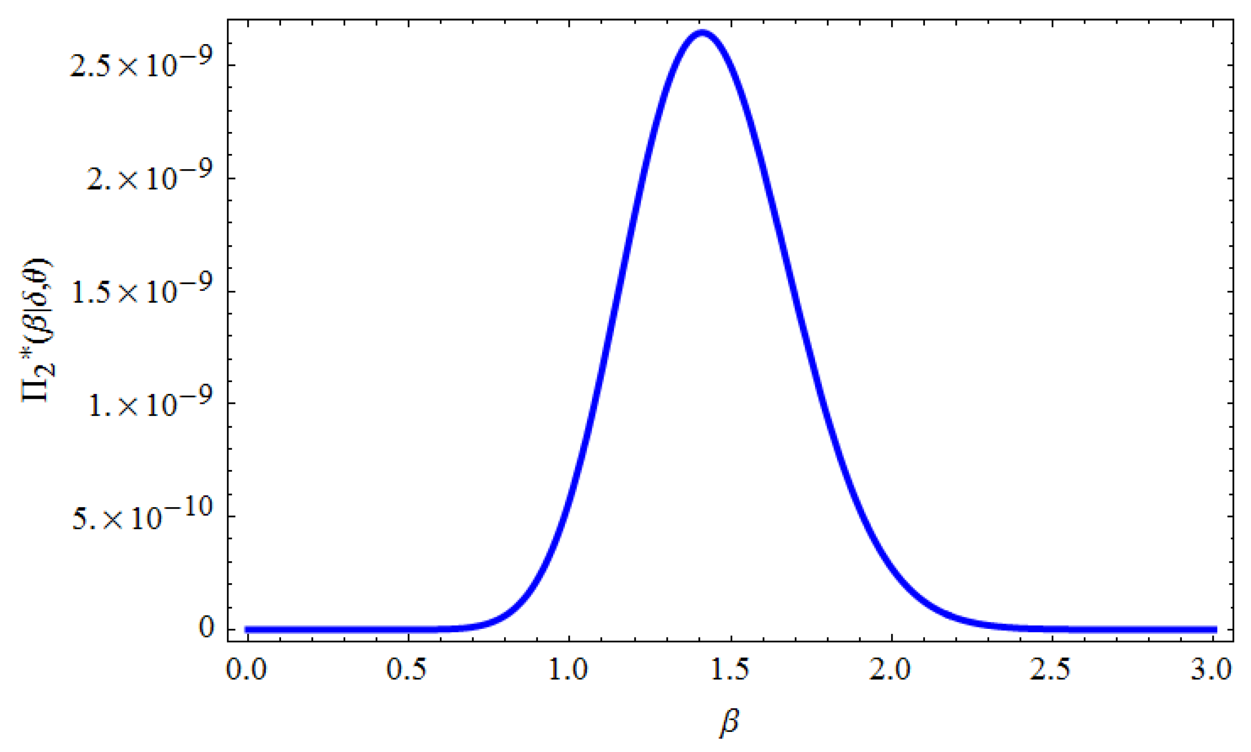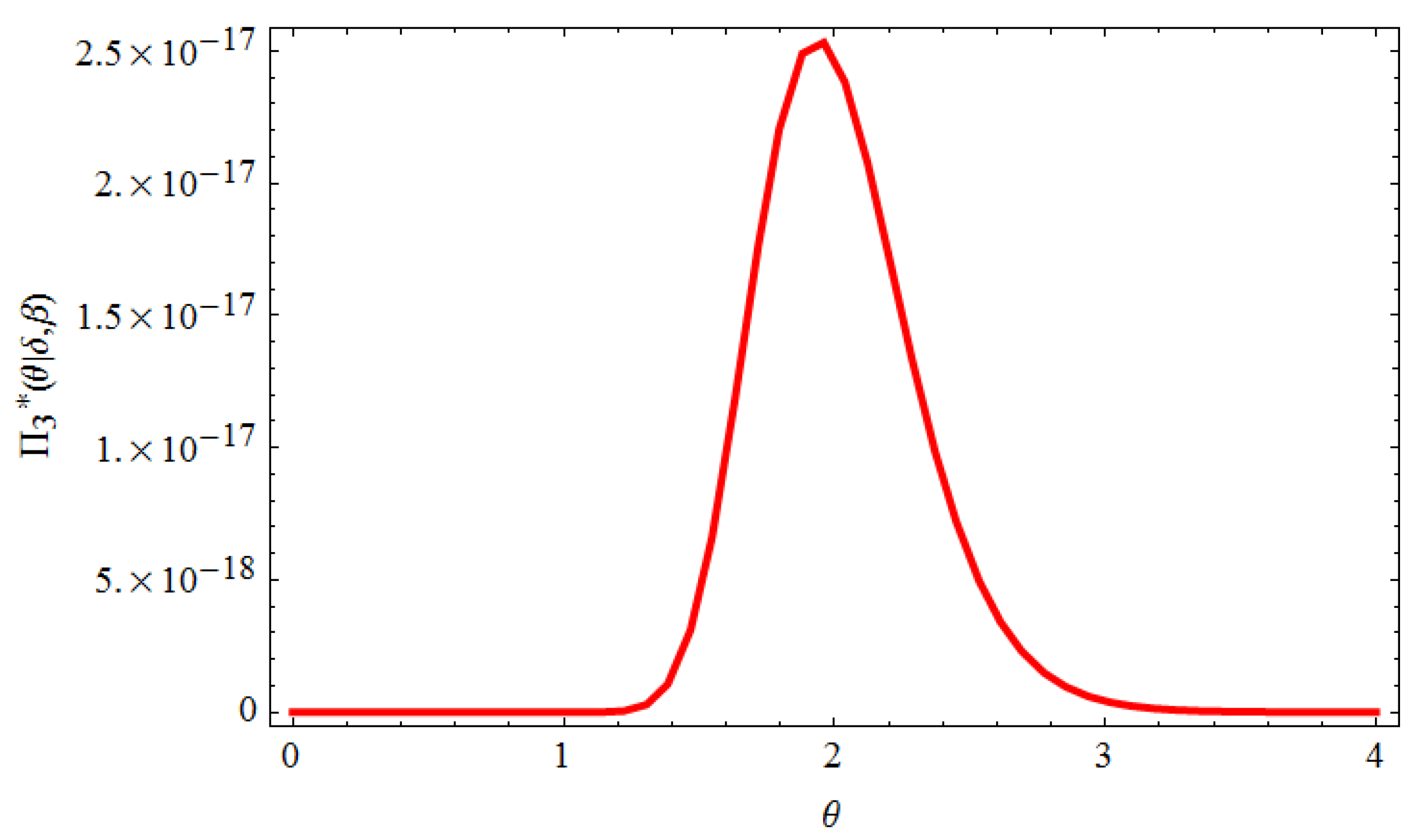[37] and later extended by Hastings [38]. In this technique, the samples can be drawn by making use of the conditional density and proposal distributions for each of the parameters. Thereafter, by using the drawn samples, the Bayes estimates and the corresponding CRIs can be computed. From (26), the conditional densities can be obtained as follows

$${\pi }_1^{*}(\delta \mid \beta ,\theta ,\underline{x})\propto {\delta }^{m+{\gamma }_1-1}exp\left\{-\delta \left[\sum _{i=1}^{m}k\left(R_i+1\right){\left(\frac{x_i}{\theta }\right)}^{\beta }+{\eta }_1\right]\right\},$$

(69)

$${\pi }_2^{*}(\beta \mid \delta ,\theta ,\underline{x})\propto {\beta }^{m+{\gamma }_2-1}\left[\prod _{i=1}^m{\left(\frac{x_i}{\theta }\right)}^{\beta -1}\right]exp\left\{-{\eta }_2\beta -\delta \left[\sum _{i=1}^{m}k\left(R_i+1\right){\left(\frac{x_i}{\theta }\right)}^{\beta }\right]\right\},$$

(70)

and

$${\pi }_3^{*}(\theta \mid \delta ,\beta ,\underline{x})\propto {\theta }^{\left(-m+{\gamma }_3-1\right)}\left[\prod _{i=1}^m{\left(\frac{x_i}{\theta }\right)}^{\beta -1}\right]exp\left\{-{\eta }_3\theta -\delta \left[\sum _{i=1}^{m}k\left(R_i+1\right){\left(\frac{x_i}{\theta }\right)}^{\beta }\right]\right\}.$$

(71)

It is noticeable that Equation (69) represents a gamma density, thus the samples of $\delta$ can be drawn simply from any gamma-generating routine. Furthermore, Equations (70) and (71) do not represent a well-known distributions. However, when plotted, they appear similar to the normal distribution, see Figure 1 and Figure 2. Consequently, the hybrid procedure of the Gibbs sampling and M-H algorithm will be run in the following steps:

Figure 1. Posterior density ${\pi }_2^{*}\left(\beta \right|\delta ,\theta ,\underline{x})$ of $\beta$.

Figure 2. Posterior density ${\pi }_3^{*}\left(\theta \right|\delta ,\beta ,\underline{x})$ of $\theta$.

(1)

Start with initial guess $\left({\delta }^{\left(0\right)},{\beta }^{\left(0\right)},{\theta }^{\left(0\right)}\right)$.

(2)

Set $j=1.$

(3)

Generate ${\delta }^{\left(j\right)}$ from gamma $\left(m+{\gamma }_1,{\eta }_1+\sum _{i=1}^{m}k\left(R_i+1\right){\left(\frac{x_i}{\theta }\right)}^{\beta }\right)$.

(4)

Using M-H to generate ${\beta }^{\left(j\right)}$ and ${\theta }^{\left(j\right)}$ from ${\pi }_2^{*}\left({\beta }^{\left(j-1\right)}\right|{\delta }^{\left(j\right)},{\theta }^{\left(j-1\right)},\underline{x})$ and ${\pi }_3^{*}\left({\theta }^{\left(j-1\right)}\right|{\delta }^{\left(j\right)},{\beta }^{\left(j\right)},\underline{x})$ with $N\left({\beta }^{\left(j-1\right)},Var\left(\beta \right)\right)$ and $N\left({\theta }^{\left(j-1\right)},Var\left(\theta \right)\right)$.

(i)

Generate ${\beta }^{*}$ from $N\left({\beta }^{\left(j-1\right)},Var\left(\beta \right)\right)$ and ${\theta }^{*}$ from $N\left({\theta }^{\left(j-1\right)},Var\left(\theta \right)\right).$

(ii)

Evaluate the acceptance probabilities

$${\psi }_{\beta }=min\left[1,\frac{{\pi }_2^{*}\left({\beta }^{*}\right|{\delta }^{\left(j\right)},{\theta }^{\left(j-1\right)},\underline{x})}{{\pi }_2^{*}\left({\beta }^{\left(j-1\right)}\right|{\delta }^{\left(j\right)},{\theta }^{\left(j-1\right)},\underline{x})}\right],{\psi }_{\theta }=min\left[1,\frac{{\pi }_3^{*}\left({\theta }^{*}\right|{\delta }^{\left(j\right)},{\beta }^{\left(j\right)},\underline{x})}{{\pi }_3^{*}\left({\theta }^{\left(j-1\right)}\right|{\delta }^{\left(j\right)},{\beta }^{\left(j\right)},\underline{x})}\right].$$

(iii)

Generate a $u_1$ and $u_2$ from a uniform $\left(0,1\right)$ distribution.

(iv)

If $u_1<{\psi }_{\beta }$ accept the proposal and set ${\beta }^{*}={\beta }^{\left(j\right)}$, else set ${\beta }^{\left(j\right)}={\beta }^{\left(j-1\right)}.$

(v)

If $u_2<{\psi }_{\theta }$ accept the proposal and set ${\theta }^{*}={\theta }^{\left(j\right)}$, else set ${\theta }^{\left(j\right)}={\theta }^{\left(j-1\right)}.$

(5)

Compute $S\left(t\right)$, $h\left(t\right)$, and $CV$ as

$\left.\begin{array}{c}{S}^{\left(j\right)}\left(t\right)=e^{-{\delta }^{\left(j\right)}{\left(\frac{t}{{\theta }^{\left(j\right)}}\right)}^{{\beta }^{\left(j\right)}}}\\ h^{\left(j\right)}\left(t\right)=\frac{{\beta }^{\left(j\right)}{\delta }^{\left(j\right)}}{{\theta }^{\left(j\right)}}{\left(\frac{t}{{\theta }^{\left(j\right)}}\right)}^{{\beta }^{\left(j\right)}-1}\\ C{V}^{\left(j\right)}=\frac{\sqrt{\mathsf{\Gamma }\left(\frac{2+{\beta }^{\left(j\right)}}{{\beta }^{\left(j\right)}}\right)-{\left[\mathsf{\Gamma }\left(\frac{1+{\beta }^{\left(j\right)}}{{\beta }^{\left(j\right)}}\right)\right]}^2}}{\mathsf{\Gamma }\left(\frac{1+{\beta }^{\left(j\right)}}{{\beta }^{\left(j\right)}}\right)}\end{array}\right\}.$

(6)

Set $j=j+1.$

(7)

Repeat Steps $3-6$ N times.

(8)

Based on BLINEX and GE loss functions, the Bayes estimate of $\upsilon$ (where $\upsilon =$$\delta ,$$\beta ,$$\theta ,$$S\left(t\right),$$h\left(t\right)$, or $CV$) under MCMC can be obtained by

$${\widehat{v}}_{BL}=\frac{-1}{c}log\left(\omega e^{-c\widehat{v}}+\frac{(1+\omega )}{N-M}\sum _{j=M+1}^N{e}^{-c{v}^{\left(j\right)}}\right),{\widehat{v}}_{GE}={\left[\frac{1}{N-M}\sum _{j=M+1}^N{\left(v^{\left(j\right)}\right)}^{-b}\right]}^{\frac{-1}{b}}.$$

where M is burn-in.

(9)

To compute the CRI of ${\upsilon }^{\left(j\right)}$, order $\left\{{\upsilon }^{M+1},{\upsilon }^{M+2},\dots ,{\upsilon }^N\right\}$ as $\left\{{\upsilon }^{\left[1\right]},{\upsilon }^{\left[2\right]},\dots ,{\upsilon }^{\left[N\right]}\right\}$. Then, the $\left(1-\gamma \right)100\%$ CRI of $\upsilon$ can be given by

$$\left[{\upsilon }_{\left(\left(N-M\right)\left(\gamma /2\right)\right)},{\upsilon }_{\left(\left(N-M\right)\left(1-\gamma /2\right)\right)}\right].$$

5. Practical Data Analysis: Gastric Cancer Patients

To clarify the inference methods discussed in the previous sections, we present a real-life example. We use a real dataset recorded in Bekker [39] that represents the survival times for a group of gastric cancer patients. Several authors have studied reliability function and associated means based on different approaches, such as Xu et al. [5] and Luo et al. [6], among others. The data consist of 46 survival times (in years) for 46 patients. The data are randomly divided into 23 groups with $(k=2)$ units within each group. The groups can be divided as follows: {0.047, 0.121}, {0.115, 1.589}, {0.466, 0.540}, {0.164, 2,444}, {0.570, 3.658}, {0.203, 0.696}, {0.841, 1.271}, {0.296, 0.334}, {0.132, 1.099}, {0.395, 0.501}, {0.260, 1.219}, {0.282, 1.326}, {0.863, 1.485}, {1.553, 2.416}, {0.458, 0.534}, {1.581, 2.830}, {0.529, 1.447}, {0.507, 2.178}, {2.343, 3.743}, {2.825, 3.578}, {0.644, 3.978}, {0.641, 4.003}, and {0.197, 4.033}. Suppose that a Pro-F-F-C scheme is given by $R=(1,0,1,0,1,0,1,0,1,0,1,0,1,0,0,0)$, then a Pro-F-F-C sample of size 16 out of 23 groups of data is obtained as follows:

0.047	0.466	0.570	0.696	0.841	1.099	1.219	1.326
1.553	1.581	1.589	2.178	2.343	2.825	4.003	4.033

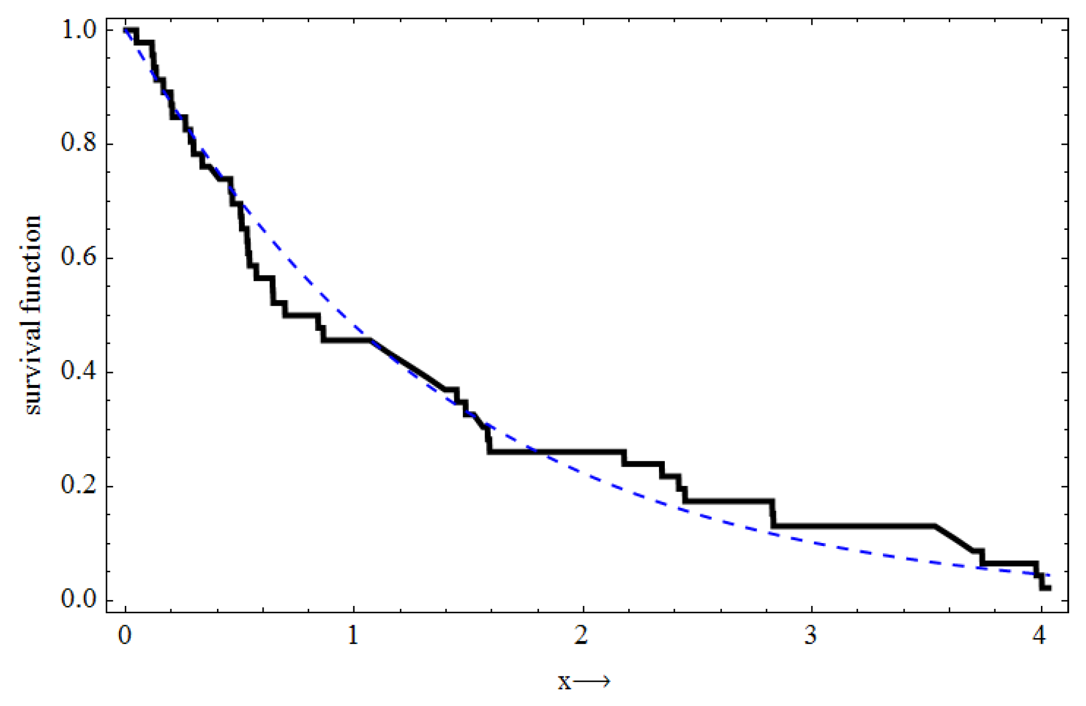
To prove that NWPD fits the data well, we computed the Kolmogorov–Smirnov and the associated p-value, and the results, respectively, are $0.1077$ and $0.6601$. From the plot of the empirical survival (ESF) and the estimated survival functions in Figure 3, it is clear that the NWPD fits the data very well. The $95\%$ CRIs of $\delta ,$$\beta$, $\theta ,$$S\left(t\right),$$h\left(t\right)$, and $CV$ are given in Table 1 and Table 2. Table 3 provides the MCMC results. Under the given previous data, we compute the MLEs of $\delta ,$$\beta ,$$\theta ,$$S\left(t\right),$$h\left(t\right)$, and $CV$ as tabulated in Table 4. Based on Lindley and MCMC techniques, Bayes estimates of $\delta ,$$\beta ,$$\theta ,$$S\left(t\right),$$h\left(t\right)$, and $CV$ with respect to BLINEX and GE loss functions are computed under gamma prior for $\delta ,$ $\beta$, and $\theta$ with hyperparameters ${\gamma }_i=4.8$ and ${\eta }_i=3.5,$ where $i=1,2,3$. 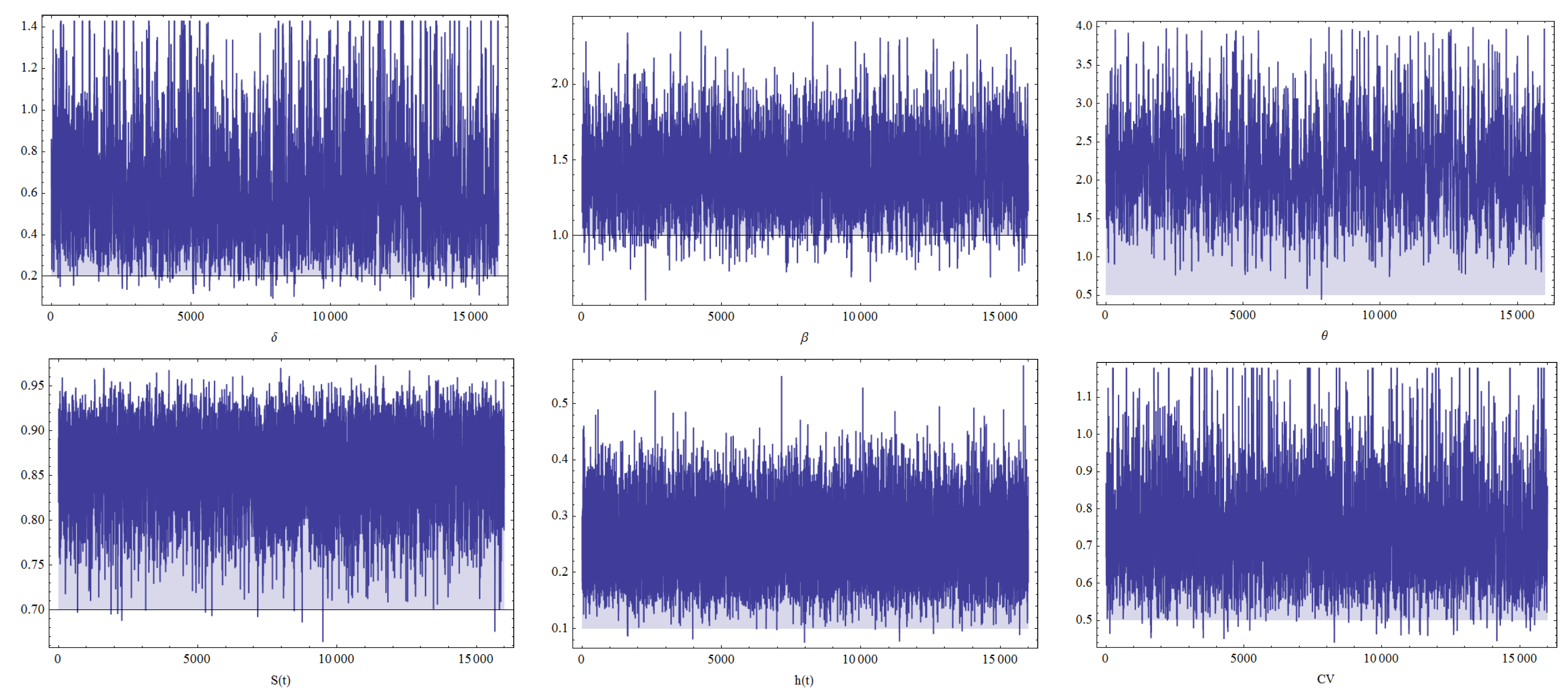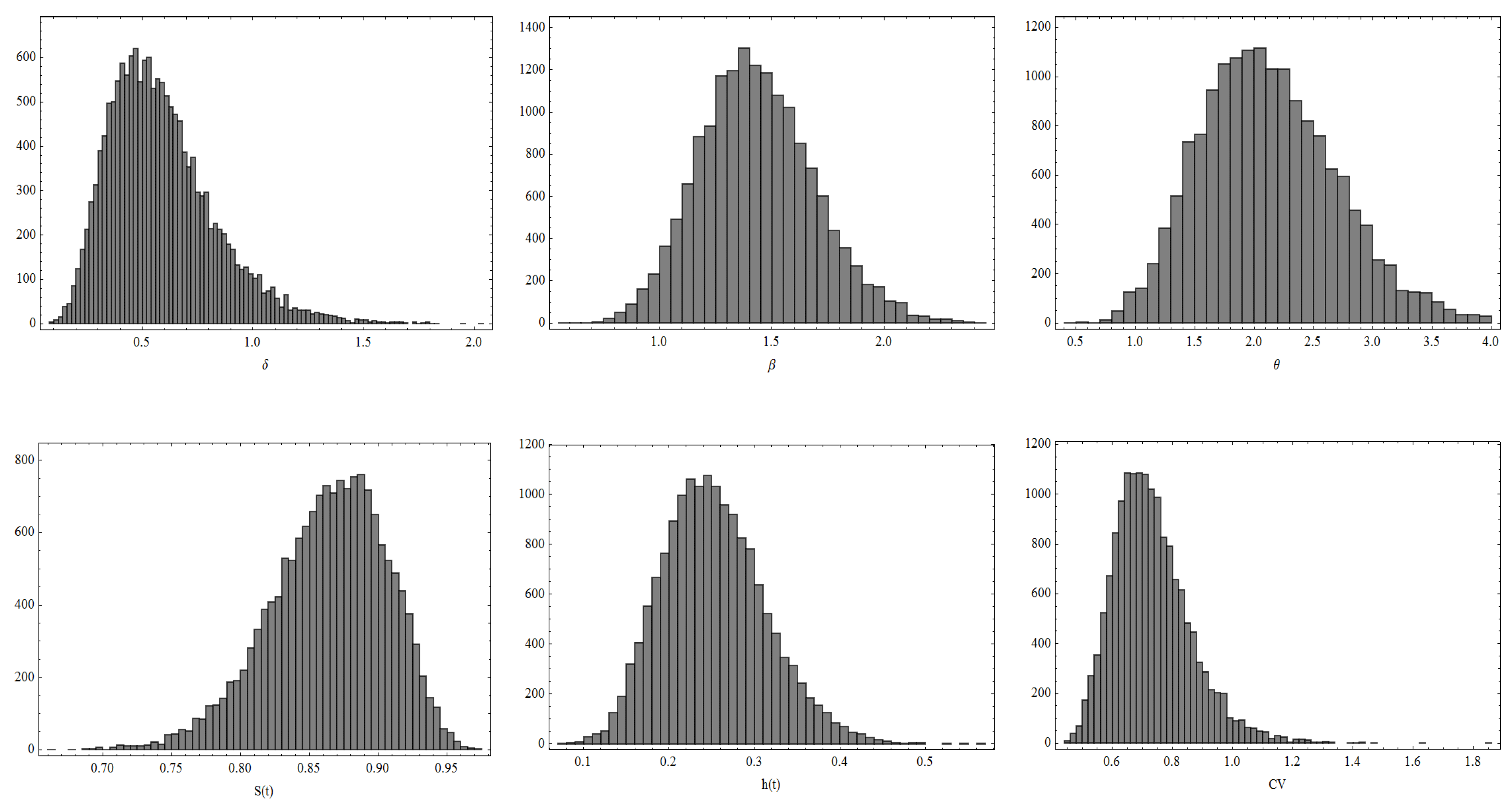Additionally, for different values of c and b, respectively, the results are reported in Table 4 and Table 5. The trace plots of the parameters generated by the MCMC approach and the associated histograms are displayed in Figure 4 and Figure 5, respectively.

Figure 3. Fitness of real data for the NWPD.

Table 1. The $95\%$ ACIs and CRIs of $\delta$, $\beta$, and $\theta$.

Parameters	ACI		CRI
	Interval	Length	Interval	Length
$\delta$	$\left[0.0701,1.1007\right]$	$1.0305$	$\left[0.2310,1.1572\right]$	$0.9261$
$\beta$	$\left[0.9379,2.0990\right]$	$1.1610$	$\left[0.9658,1.9753\right]$	$1.0095$
$\theta$	$\left[1.2278,3.5054\right]$	$2.2776$	$\left[1.1282,3.3612\right]$	$2.2330$

Table 2. The $95\%$ ACIs, $\mathcal{L}$TCIs, ASTCIs, and CRIs of $S\left(t\right)$, $h\left(t\right)$, and $CV$.

Parameters	ACI		$\mathcal{L}$TCI
	Interval	Length	Interval	Length
$S\left(t=0.8\right)$	$\left[0.8152,0.9715\right]$	$0.1563$	$\left[0.8010,0.9457\right]$	$0.1447$
$h\left(t=0.8\right)$	$\left[0.0992,0.3289\right]$	$0.2298$	$\left[0.1905,0.2397\right]$	$0.0492$
$CV$	$\left[0.4352,0.9076\right]$	$0.4724$	$\left[0.4989,0.8074\right]$	$0.3085$
	ASTCI		CRI
	Interval	Length	Interval	Length
$S\left(t=0.8\right)$	$\left[0.8035,0.9581\right]$	$0.1546$	$\left[0.7704,0.9353\right]$	$0.1649$
$h\left(t=0.8\right)$	$\left[0.1118,0.3386\right]$	$0.2268$	$\left[0.1482,0.3825\right]$	$0.2344$
$CV$	$\left[0.4238,0.8765\right]$	$0.4527$	$\left[0.5286,1.0355\right]$	$0.5069$

Table 3. MCMC results of $\delta$, $\beta$, $\theta$, $S\left(t\right)$, $h\left(t\right)$, and $CV$.

Parameters	Mean	Median	Mode	SD	Ske
$\delta$	$0.5860$	$0.5486$	$0.4737$	$0.2402$	$0.9847$
$\beta$	$1.4318$	$1.4189$	$1.3932$	$0.2553$	$0.2845$
$\theta$	$2.1188$	$2.0756$	$1.9892$	$0.5689$	$0.3694$
$S\left(t=0.8\right)$	$0.8639$	$0.8675$	$0.8747$	$0.0426$	$-0.5053$
$h\left(t=0.8\right)$	$0.2523$	$0.2480$	$0.2394$	$0.0603$	$0.4140$
$CV$	$0.7319$	$0.7148$	$0.6805$	$0.1295$	$1.0006$

Table 4. MLEs and Bayes Lindley estimates of $\delta$, $\beta$, $\theta$, $S\left(t\right)$, $h\left(t\right)$, and $CV$ under BLINEX and GE loss functions with $t=0.8$.

$\left(.\right)$	${\left(.\right)}_{\mathit{ML}}$	${\left(.\right)}_{\mathit{Lindley}}$
		$\mathit{\omega }$	${\left(.\right)}_{\mathit{BL}}$					${\left(.\right)}_{\mathit{GE}}$
			$\mathit{c}=-\mathbf{3}$	$\mathit{c}=-\mathbf{1}$	$\mathit{c}=\mathbf{0.001}$	$\mathit{c}=\mathbf{1}$	$\mathit{c}=\mathbf{3}$	$\mathit{b}=-\mathbf{2}$	$\mathit{b}=\mathbf{1}$
$\delta$	$0.5854$	$0.0$	$0.6665$	$0.6535$	$0.6451$	$0.6357$	$0.6142$	$0.6588$	$0.6095$
		$0.3$	$0.6442$	$0.6335$	$0.6272$	$0.6203$	$0.6053$
		$0.6$	$0.6202$	$0.6132$	$0.6093$	$0.6052$	$0.5966$
		$0.9$	$0.5945$	$0.5924$	$0.5914$	$0.5903$	$0.5882$
$\beta$	$1.5184$	$0.0$	$1.5202$	$1.4289$	$1.389$	$1.3588$	$1.3259$	$1.4142$	$1.352$
		$0.3$	$1.5197$	$1.4566$	$1.4279$	$1.4041$	$1.3730$
		$0.6$	$1.5191$	$1.4836$	$1.4667$	$1.4515$	$1.4278$
		$0.9$	$1.5186$	$1.5098$	$1.5055$	$1.5013$	$1.4934$
$\theta$	$2.3666$	$0.0$	$2.4015$	$2.2444$	$2.1756$	$2.1300$	$2.0954$	$2.202$	$2.1363$
		$0.3$	$2.3914$	$2.2826$	$2.2329$	$2.1953$	$2.1563$
		$0.6$	$2.3810$	$2.3195$	$2.2902$	$2.2652$	$2.2309$
		$0.9$	$2.3702$	$2.3550$	$2.3475$	$2.3403$	$2.3271$
$S\left(t\right)$	$0.8934$	0	$0.848$	$0.8476$	$0.8475$	$0.8474$	$0.8473$	$0.8476$	$0.8474$
		$0.3$	$0.8623$	$0.8616$	$0.8612$	$0.861$	$0.8605$
		$0.6$	$0.8759$	$0.8753$	$0.875$	$0.8747$	$0.8742$
		$0.9$	$0.8891$	$0.8889$	$0.8888$	$0.8887$	$0.8885$
$h\left(t\right)$	$0.2141$	0	$0.2844$	$0.2834$	$0.2827$	$0.2817$	$0.2789$	$0.2857$	$0.2609$
		$0.3$	$0.2648$	$0.2631$	$0.2621$	$0.2609$	$0.2581$
		$0.6$	$0.244$	$0.2424$	$0.2415$	$0.2405$	$0.2385$
		$0.9$	$0.2218$	$0.2212$	$0.2209$	$0.2206$	$0.22$
$CV$	$0.6714$	$0.0$	$0.7575$	$0.7518$	$0.7479$	$0.7432$	$0.7313$	$0.7537$	$0.7313$
		$0.3$	$0.7339$	$0.7284$	$0.7250$	$0.7211$	$0.7122$
		$0.6$	$0.7085$	$0.7043$	$0.7020$	$0.6995$	$0.6941$
		$0.9$	$0.6811$	$0.6797$	$0.6790$	$0.6783$	$0.6769$

Table 5. Bayes MCMC estimates of $\delta$, $\beta$, $\theta$, $S\left(t\right)$, $h\left(t\right)$, and $CV$ under BLINEX and GE loss functions with $t=0.8$.

$\left(.\right)$	${\left(.\right)}_{\mathit{MCMC}}$
	$\mathit{\omega }$	${\left(.\right)}_{\mathit{BL}}$					${\left(.\right)}_{\mathit{GE}}$
		$\mathit{c}=-\mathbf{3}$	$\mathit{c}=-\mathbf{1}$	$\mathit{c}=\mathbf{0.001}$	$\mathit{c}=\mathbf{1}$	$\mathit{c}=\mathbf{3}$	$\mathit{b}=-\mathbf{1}$	$\mathit{b}=\mathbf{1}$
$\delta$	$0.0$	$0.6997$	$0.6174$	$0.5860$	$0.5593$	$0.5156$	$0.6333$	$0.4941$
	$0.3$	$0.6693$	$0.6079$	$0.5858$	$0.5670$	$0.5351$
	$0.6$	$0.6359$	$0.5983$	$0.5856$	$0.5749$	$0.5557$
	$0.9$	$0.5988$	$0.5886$	$0.5855$	$0.5827$	$0.5777$
$\beta$	$0.0$	$1.5367$	$1.4652$	$1.4317$	$1.4000$	$1.3407$	$1.4544$	$1.3857$
	$0.3$	$1.5313$	$1.4814$	$1.4578$	$1.4341$	$1.3848$
	$0.6$	$1.5259$	$1.4975$	$1.4838$	$1.4694$	$1.4357$
	$0.9$	$1.5203$	$1.5132$	$1.5098$	$1.5059$	$1.4958$
$\theta$	$0.0$	$2.6651$	$2.2913$	$2.1187$	$1.9684$	$1.7286$	$2.1939$	$1.9606$
	$0.3$	$2.6000$	$2.3145$	$2.1930$	$2.0722$	$1.8270$
	$0.6$	$2.5190$	$2.3371$	$2.2674$	$2.1879$	$1.9674$
	$0.9$	$2.4117$	$2.3593$	$2.3418$	$2.3188$	$2.2145$
$S\left(t\right)$	0	$0.8665$	$0.8648$	$0.8638$	$0.8629$	$0.8611$	$0.8649$	$0.8617$
	$0.3$	$0.8748$	$0.8734$	$0.8727$	$0.872$	$0.8704$
	$0.6$	$0.8829$	$0.8820$	$0.8816$	$0.8811$	$0.8801$
	$0.9$	$0.8908$	$0.8905$	$0.8904$	$0.8903$	$0.8900$
$h\left(t\right)$	$0.0$	$0.2579$	$0.2542$	$0.2523$	$0.2505$	$0.2470$	$0.2594$	$0.2377$
	$0.3$	$0.2453$	$0.2423$	$0.2408$	$0.2394$	$0.2368$
	$0.6$	$0.2323$	$0.2303$	$0.2294$	$0.2285$	$0.2268$
	$0.9$	$0.2187$	$0.2181$	$0.2179$	$0.2176$	$0.2172$
$CV$	$0.0$	$0.7614$	$0.7407$	$0.7319$	$0.7239$	$0.7095$	$0.7433$	$0.7111$
	$0.3$	$0.7369$	$0.7204$	$0.7138$	$0.7078$	$0.6976$
	$0.6$	$0.7104$	$0.6997$	$0.6956$	$0.692$	$0.6861$
	$0.9$	$0.6816$	$0.6785$	$0.6774$	$0.6765$	$0.6750$

Figure 4. Trace plots of $\delta$, $\beta$, $\theta$, $S\left(t\right)$, $h\left(t\right)$, and $CV$ obtained from the MCMC approach.

Figure 5. Histogram of $\delta$, $\beta$, $\theta$, $S\left(t\right)$, $h\left(t\right)$, and $CV$ of the MCMC approach.

6. Monte Carlo Simulation Study

In our diligent quest to evaluate the performance of the inference methods proposed in this article, some computations are made according to Monte Carlo simulation experiments using MATHEMATICA version 12 with different combinations of n, m, and k and different censored scheme R (different $R_i$ values). Using the algorithm introduced by Balakrishnan and Sandhu [3], with distribution function $1-{\left(1-F\left(x\right)\right)}^k$, we generate a Pro-F-F-C sample from the NWPD with the parameters $\delta ,\beta ,$ and $\theta =0.5,1.5,$ and 1, respectively. The true values of $S\left(t\right)$, $h\left(t\right)$, and $CV$ at time $t=0.3$ are evaluated to be $S\left(t\right)=0.9211$, $h\left(t\right)=0.4108$, and $CV=0.679$. The performance of the resulting estimators of $\delta ,$$\beta ,$$\theta ,$$S\left(t\right),$$h\left(t\right)$, and $CV$ have been considered in terms of their average mean (AVM) and the corresponding mean squared error (MSE), which are computed, for $k=1,2,\dots ,6$ and ${\varphi }_1=\delta$, ${\varphi }_2=\beta$, ${\varphi }_3=\theta$, ${\varphi }_4=S\left(t\right)$, ${\varphi }_5=h\left(t\right)$ and ${\varphi }_6=CV$ as $AVM=\frac{1}{M}\sum _{j=1}^M{\widehat{\varphi }}_k^{\left(j\right)}$, and $MSE=\frac{1}{M}\sum _{j=1}^M{\left({\widehat{\varphi }}_k^{\left(j\right)}-{\varphi }_k\right)}^2$. Additionally, we compare different CIs obtained by using asymptotic distributions of the MLEs, the delta method, and symmetric CRIs, which were made in terms of the average CI, CRI lengths, and coverage percentages (CPs). Under the consideration of informative gamma priors for $\delta$, $\beta$, and $\theta$ with hyperparameters ${\gamma }_1=5,$${\eta }_1=5,{\gamma }_2=6,{\eta }_2$$=4$$,{\gamma }_3=6$, and ${\eta }_3$$=5$, the Bayes estimators using Lindley and MCMC have been obtained. Moreover, Bayes estimates are obtained under BLINEX and GE loss functions for the choice $c=-1,1$ with $\omega =0.3,0.9$ and $b=-2,-1,1$, respectively. In our study, we adopted two different groups $k=2,6$, and the following CS:

CS I: $R_1=n-m,R_i=0$ for $i\ne 1.$

CS II: $R_{\frac{m}{2}}=\frac{m}{2},R_i=0$ for $i\ne \frac{m}{2}.$

CS III: $R_m=n-m,R_i=0$ for $i\ne m.$

The results of the AVM and MSE of estimates are listed in Table 6, Table 7, Table 8, Table 9, Table 10 and Table 11, while the results of the ACI, CRI lengths, and CPS of the estimates are shown in Table 12.

Table 6. Average mean and MSE of estimates for the parameter $\delta$.

k	(n,m)	CS	MLE	Lindley
				$(\mathbf{\omega }=\mathbf{0.3})$		$(\mathbf{\omega }=\mathbf{0.9})$
				BLINEX		BLINEX		GE
				$\mathbf{c}=-\mathbf{1}$	$\mathbf{c}=\mathbf{1}$	$\mathbf{c}=-\mathbf{1}$	$\mathbf{c}=\mathbf{1}$	$\mathbf{b}=-\mathbf{2}$	$\mathbf{b}=-\mathbf{1}$	$\mathbf{b}=\mathbf{1}$
2	(30,20)	I	0.5622	0.5802	0.5682	0.5648	0.563	0.5912	0.5792	0.5538
			$\left(0.0602\right)$	$\left(0.0535\right)$	$\left(0.0475\right)$	$\left(0.0592\right)$	$\left(0.0582\right)$	$\left(0.0511\right)$	$\left(0.0466\right)$	$\left(0.0403\right)$
		II	0.5754	0.5922	0.5797	0.5778	0.5759	0.6027	0.5904	0.5645
			$\left(0.0643\right)$	$\left(0.0569\right)$	$\left(0.0503\right)$	$\left(0.0631\right)$	$\left(0.062\right)$	$\left(0.0543\right)$	$\left(0.0494\right)$	$\left(0.0425\right)$
		III	0.5833	0.5987	0.5857	0.5856	0.5836	0.6079	0.5957	0.5705
			$\left(0.0815\right)$	$\left(0.0701\right)$	$\left(0.0622\right)$	$\left(0.0797\right)$	$\left(0.0784\right)$	$\left(0.0655\right)$	$\left(0.06\right)$	$\left(0.0525\right)$
	(40,30)	I	0.5479	0.5617	0.5541	0.5499	0.5487	0.5704	0.5622	0.5448
			$\left(0.0468\right)$	$\left(0.0436\right)$	$\left(0.0403\right)$	$\left(0.0463\right)$	$\left(0.0458\right)$	$\left(0.0425\right)$	$\left(0.04\right)$	$\left(0.0362\right)$
		II	0.5765	0.5879	0.5793	0.5781	0.5768	0.5952	0.5866	0.5688
			$\left(0.0642\right)$	$\left(0.0586\right)$	$\left(0.054\right)$	$\left(0.0634\right)$	$\left(0.0626\right)$	$\left(0.0563\right)$	$\left(0.0531\right)$	$\left(0.048\right)$
		III	0.5719	0.5839	0.5754	0.5736	0.5724	0.5914	0.5829	0.5654
			$\left(0.0685\right)$	$\left(0.0622\right)$	$\left(0.0573\right)$	$\left(0.0675\right)$	$\left(0.0667\right)$	$\left(0.0595\right)$	$\left(0.0562\right)$	$\left(0.0511\right)$
6	(30,20)	I	0.609	0.6201	0.6063	0.6107	0.6085	0.6276	0.6147	0.5886
			$\left(0.0856\right)$	$\left(0.0723\right)$	$\left(0.0639\right)$	$\left(0.0837\right)$	$\left(0.0821\right)$	$\left(0.0669\right)$	$\left(0.0611\right)$	$\left(0.0532\right)$
		II	0.629	0.6379	0.6231	0.6304	0.6281	0.6444	0.6308	0.604
			$\left(0.0915\right)$	$\left(0.0782\right)$	$\left(0.0687\right)$	$\left(0.0895\right)$	$\left(0.0878\right)$	$\left(0.0727\right)$	$\left(0.0661\right)$	$\left(0.057\right)$
		III	0.6417	0.648	0.6327	0.6427	0.6403	0.6531	0.6394	0.6128
			$\left(0.1044\right)$	$\left(0.0873\right)$	$\left(0.0769\right)$	$\left(0.1019\right)$	$\left(0.0999\right)$	$\left(0.08\right)$	$\left(0.073\right)$	$\left(0.0637\right)$
	(40,30)	I	0.6012	0.6096	0.6003	0.6025	0.601	0.6154	0.6064	0.5883
			$\left(0.08\right)$	$\left(0.0715\right)$	$\left(0.0657\right)$	$\left(0.0788\right)$	$\left(0.0778\right)$	$\left(0.0678\right)$	$\left(0.0639\right)$	$\left(0.058\right)$
		II	0.6133	0.6207	0.611	0.6144	0.6129	0.6261	0.6168	0.5983
			$\left(0.0829\right)$	$\left(0.0746\right)$	$\left(0.0685\right)$	$\left(0.0817\right)$	$\left(0.0807\right)$	$\left(0.0711\right)$	$\left(0.0668\right)$	$\left(0.0604\right)$
		III	0.6334	0.6393	0.629	0.6343	0.6327	0.6439	0.6343	0.6154
			$\left(0.0938\right)$	$\left(0.0842\right)$	$\left(0.0772\right)$	$\left(0.0924\right)$	$\left(0.0912\right)$	$\left(0.08\right)$	$\left(0.0753\right)$	$\left(0.0679\right)$
k	(n,m)	CS		MCMC
				$(\mathbf{\omega }=\mathbf{0.3})$		$(\mathbf{\omega }=\mathbf{0.9})$
				BLINEX		BLINEX		GE
				$\mathbf{c}=-\mathbf{1}$	$\mathbf{c}=\mathbf{1}$	$\mathbf{c}=-\mathbf{1}$	$\mathbf{c}=\mathbf{1}$	$\mathbf{b}=-\mathbf{2}$	$\mathbf{b}=-\mathbf{1}$	$\mathbf{b}=\mathbf{1}$
2	(30,20)	I		0.6422	0.5977	0.5764	0.5647	0.6721	0.6435	0.5806
				$\left(0.0244\right)$	$\left(0.0127\right)$	$\left(0.0501\right)$	$\left(0.0472\right)$	$\left(0.0346\right)$	$\left(0.025\right)$	$\left(0.0101\right)$
		II		0.6419	0.5978	0.5875	0.576	0.6666	0.6376	0.5749
				$\left(0.0245\right)$	$\left(0.0128\right)$	$\left(0.0539\right)$	$\left(0.0504\right)$	$\left(0.0321\right)$	$\left(0.0229\right)$	$\left(0.0087\right)$
		III		0.6497	0.6003	0.5959	0.5826	0.6722	0.6412	0.5755
				$\left(0.0287\right)$	$\left(0.0146\right)$	$\left(0.0686\right)$	$\left(0.0638\right)$	$\left(0.0342\right)$	$\left(0.024\right)$	$\left(0.0089\right)$
	(40,30)	I		0.5704	0.5419	0.5528	0.545	0.5787	0.5591	0.5151
				$\left(0.0091\right)$	$\left(0.0044\right)$	$\left(0.0385\right)$	$\left(0.0356\right)$	$\left(0.0102\right)$	$\left(0.0072\right)$	$\left(0.0034\right)$
		II		0.5786	0.5471	0.5788	0.5695	0.5757	0.5563	0.5128
				$\left(0.0115\right)$	$\left(0.0052\right)$	$\left(0.0536\right)$	$\left(0.0484\right)$	$\left(0.0094\right)$	$\left(0.0066\right)$	$\left(0.0031\right)$
		III		0.5752	0.5429	0.5744	0.5649	0.5725	0.5527	0.5086
				$\left(0.0119\right)$	$\left(0.0054\right)$	$\left(0.0573\right)$	$\left(0.0517\right)$	$\left(0.0086\right)$	$\left(0.0059\right)$	$\left(0.0026\right)$
6	(30,20)	I		0.6704	0.6161	0.6209	0.6068	0.6908	0.6558	0.5833
				$\left(0.0342\right)$	$\left(0.0169\right)$	$\left(0.0731\right)$	$\left(0.0673\right)$	$\left(0.0406\right)$	$\left(0.0279\right)$	$\left(0.0097\right)$
		II		0.6809	0.6235	0.6396	0.6249	0.6972	0.6598	0.583
				$\left(0.0372\right)$	$\left(0.0184\right)$	$\left(0.0785\right)$	$\left(0.0723\right)$	$\left(0.043\right)$	$\left(0.0291\right)$	$\left(0.0095\right)$
		III		0.7102	0.6411	0.655	0.6381	0.7323	0.6865	0.5964
				$\left(0.05\right)$	$\left(0.0242\right)$	$\left(0.0908\right)$	$\left(0.0834\right)$	$\left(0.0578\right)$	$\left(0.0381\right)$	$\left(0.0119\right)$
	(40,30)	I		0.5965	0.5583	0.6029	0.5917	0.5892	0.566	0.5163
				$\left(0.0151\right)$	$\left(0.0061\right)$	$\left(0.0673\right)$	$\left(0.0601\right)$	$\left(0.0112\right)$	$\left(0.0073\right)$	$\left(0.0026\right)$
		II		0.6037	0.5637	0.6143	0.6027	0.5945	0.5698	0.5173
				$\left(0.0161\right)$	$\left(0.0067\right)$	$\left(0.0698\right)$	$\left(0.0626\right)$	$\left(0.0123\right)$	$\left(0.0079\right)$	$\left(0.0026\right)$
		III		0.6257	0.5795	0.635	0.622	0.6174	0.5878	0.5274
				$\left(0.0217\right)$	$\left(0.0095\right)$	$\left(0.0796\right)$	$\left(0.0716\right)$	$\left(0.0172\right)$	$\left(0.0107\right)$	$\left(0.0031\right)$

Table 7. Average mean and MSE of estimates for the parameter $\beta$.

k	(n,m)	CS	MLE	Lindley
				$(\mathbf{\omega }=\mathbf{0.3})$		$(\mathbf{\omega }=\mathbf{0.9})$
				BLINEX		BLINEX		GE
				$\mathbf{c}=-\mathbf{1}$	$\mathbf{c}=\mathbf{1}$	$\mathbf{c}=-\mathbf{1}$	$\mathbf{c}=\mathbf{1}$	$\mathbf{b}=-\mathbf{2}$	$\mathbf{b}=-\mathbf{1}$	$\mathbf{b}=\mathbf{1}$
2	(30,20)	I	1.567	1.5331	1.4952	1.5623	1.5563	1.5072	1.4899	1.4602
			$\left(0.06\right)$	$\left(0.041\right)$	$\left(0.0387\right)$	$\left(0.0571\right)$	$\left(0.0559\right)$	$\left(0.0324\right)$	$\left(0.0329\right)$	$\left(0.036\right)$
		II	1.561	1.5318	1.4937	1.557	1.551	1.5079	1.4904	1.4603
			$\left(0.0615\right)$	$\left(0.0413\right)$	$\left(0.0385\right)$	$\left(0.0584\right)$	$\left(0.0571\right)$	$\left(0.0319\right)$	$\left(0.0322\right)$	$\left(0.0351\right)$
		III	1.5746	1.5466	1.4924	1.5709	1.5622	1.5173	1.4929	1.4522
			$\left(0.071\right)$	$\left(0.0418\right)$	$\left(0.0357\right)$	$\left(0.0666\right)$	$\left(0.0639\right)$	$\left(0.0275\right)$	$\left(0.0271\right)$	$\left(0.0309\right)$
	(40,30)	I	1.5509	1.5281	1.5014	1.5477	1.5437	1.5108	1.4984	1.4763
			$\left(0.0426\right)$	$\left(0.0332\right)$	$\left(0.0313\right)$	$\left(0.0412\right)$	$\left(0.0405\right)$	$\left(0.0285\right)$	$\left(0.0285\right)$	$\left(0.0295\right)$
		II	1.5287	1.5104	1.4837	1.5261	1.5221	1.4953	1.4828	1.4602
			$\left(0.0388\right)$	$\left(0.0303\right)$	$\left(0.0291\right)$	$\left(0.0375\right)$	$\left(0.037\right)$	$\left(0.0262\right)$	$\left(0.0264\right)$	$\left(0.0279\right)$
		III	1.5505	1.5336	1.4968	1.5482	1.5426	1.5158	1.4989	1.4687
			$\left(0.0491\right)$	$\left(0.0357\right)$	$\left(0.032\right)$	$\left(0.0471\right)$	$\left(0.046\right)$	$\left(0.0285\right)$	$\left(0.0279\right)$	$\left(0.0291\right)$
6	(30,20)	I	1.5214	1.5254	1.4923	1.522	1.5171	1.5181	1.5029	1.4743
			$\left(0.0319\right)$	$\left(0.025\right)$	$\left(0.0209\right)$	$\left(0.0309\right)$	$\left(0.03\right)$	$\left(0.0204\right)$	$\left(0.0191\right)$	$\left(0.0185\right)$
		II	1.5083	1.5155	1.4895	1.5094	1.5055	1.5117	1.4997	1.4766
			$\left(0.0267\right)$	$\left(0.0221\right)$	$\left(0.0191\right)$	$\left(0.026\right)$	$\left(0.0255\right)$	$\left(0.0189\right)$	$\left(0.0178\right)$	$\left(0.0171\right)$
		III	1.5137	1.5219	1.4948	1.5149	1.5109	1.518	1.5057	1.4821
			$\left(0.0286\right)$	$\left(0.0239\right)$	$\left(0.0197\right)$	$\left(0.0279\right)$	$\left(0.0272\right)$	$\left(0.0202\right)$	$\left(0.0187\right)$	$\left(0.0171\right)$
	(40,30)	I	1.5077	1.5107	1.4878	1.5081	1.5048	1.506	1.4954	1.475
			$\left(0.0247\right)$	$\left(0.021\right)$	$\left(0.0188\right)$	$\left(0.0241\right)$	$\left(0.0237\right)$	$\left(0.0185\right)$	$\left(0.0178\right)$	$\left(0.0173\right)$
		II	1.4995	1.5041	1.485	1.5002	1.4974	1.5012	1.4923	1.4751
			$\left(0.0221\right)$	$\left(0.0193\right)$	$\left(0.0175\right)$	$\left(0.0217\right)$	$\left(0.0213\right)$	$\left(0.0173\right)$	$\left(0.0167\right)$	$\left(0.0163\right)$
		III	1.4968	1.5027	1.483	1.4977	1.4948	1.5001	1.491	1.4733
			$\left(0.0226\right)$	$\left(0.0197\right)$	$\left(0.0176\right)$	$\left(0.0222\right)$	$\left(0.0218\right)$	$\left(0.0177\right)$	$\left(0.0169\right)$	$\left(0.0161\right)$
k	(n,m)	CS		MCMC
				$(\mathbf{\omega }=\mathbf{0.3})$		$(\mathbf{\omega }=\mathbf{0.9})$
				BLINEX		BLINEX		GE
				$\mathbf{c}=-\mathbf{1}$	$\mathbf{c}=\mathbf{1}$	$\mathbf{c}=-\mathbf{1}$	$\mathbf{c}=\mathbf{1}$	$\mathbf{b}=-\mathbf{2}$	$\mathbf{b}=-\mathbf{1}$	$\mathbf{b}=\mathbf{1}$
2	(30,20)	I		1.5568	1.5169	1.5656	1.5595	1.5416	1.5238	1.4877
				$\left(0.0458\right)$	$\left(0.0383\right)$	$\left(0.0579\right)$	$\left(0.0561\right)$	$\left(0.0373\right)$	$\left(0.0353\right)$	$\left(0.0333\right)$
		II		1.5595	1.5209	1.5609	1.5551	1.5484	1.5312	1.496
				$\left(0.0483\right)$	$\left(0.0404\right)$	$\left(0.0596\right)$	$\left(0.0578\right)$	$\left(0.0399\right)$	$\left(0.0377\right)$	$\left(0.0351\right)$
		III		1.5942	1.5396	1.5776	1.5694	1.5867	1.5629	1.5143
				$\left(0.0554\right)$	$\left(0.0424\right)$	$\left(0.0686\right)$	$\left(0.066\right)$	$\left(0.0445\right)$	$\left(0.04\right)$	$\left(0.0345\right)$
	(40,30)	I		1.5381	1.5098	1.5492	1.5449	1.5252	1.5124	1.4864
				$\left(0.0344\right)$	$\left(0.0305\right)$	$\left(0.0414\right)$	$\left(0.0405\right)$	$\left(0.0297\right)$	$\left(0.0287\right)$	$\left(0.0277\right)$
		II		1.5241	1.497	1.528	1.5241	1.5152	1.5027	1.4775
				$\left(0.0327\right)$	$\left(0.0298\right)$	$\left(0.0379\right)$	$\left(0.0372\right)$	$\left(0.029\right)$	$\left(0.0283\right)$	$\left(0.0279\right)$
		III		1.5574	1.5203	1.5515	1.5461	1.5502	1.5335	1.4998
				$\left(0.0405\right)$	$\left(0.0341\right)$	$\left(0.0478\right)$	$\left(0.0466\right)$	$\left(0.0345\right)$	$\left(0.0325\right)$	$\left(0.0301\right)$
6	(30,20)	I		1.5655	1.5274	1.5278	1.5222	1.5734	1.5564	1.5221
				$\left(0.0308\right)$	$\left(0.025\right)$	$\left(0.0314\right)$	$\left(0.0308\right)$	$\left(0.0289\right)$	$\left(0.0262\right)$	$\left(0.0225\right)$
		II		1.5574	1.5224	1.5155	1.5103	1.5684	1.5528	1.5211
				$\left(0.0264\right)$	$\left(0.0217\right)$	$\left(0.0263\right)$	$\left(0.0259\right)$	$\left(0.0255\right)$	$\left(0.0232\right)$	$\left(0.0199\right)$
		III		1.5983	1.5491	1.5263	1.5187	1.6187	1.5979	1.5556
				$\left(0.0328\right)$	$\left(0.0234\right)$	$\left(0.0283\right)$	$\left(0.0277\right)$	$\left(0.0342\right)$	$\left(0.0292\right)$	$\left(0.0218\right)$
	(40,30)	I		1.5427	1.515	1.5128	1.5087	1.5501	1.5375	1.5122
				$\left(0.0243\right)$	$\left(0.0212\right)$	$\left(0.0244\right)$	$\left(0.0241\right)$	$\left(0.0234\right)$	$\left(0.0219\right)$	$\left(0.02\right)$
		II		1.5387	1.5126	1.5052	1.5014	1.5482	1.5364	1.5125
				$\left(0.0217\right)$	$\left(0.019\right)$	$\left(0.0218\right)$	$\left(0.0216\right)$	$\left(0.0212\right)$	$\left(0.0198\right)$	$\left(0.0181\right)$
		III		1.5636	1.528	1.5066	1.5012	1.5814	1.5659	1.5346
				$\left(0.0243\right)$	$\left(0.0195\right)$	$\left(0.0223\right)$	$\left(0.022\right)$	$\left(0.0252\right)$	$\left(0.0226\right)$	$\left(0.0188\right)$

Table 8. Average mean and MSE of estimates for the parameter $\theta$.

k	(n,m)	CS	MLE	Lindley
				$(\mathbf{\omega }=\mathbf{0.3})$		$(\mathbf{\omega }=\mathbf{0.9})$
				BLINEX		BLINEX		GE
				$\mathbf{c}=-\mathbf{1}$	$\mathbf{c}=\mathbf{1}$	$\mathbf{c}=-\mathbf{1}$	$\mathbf{c}=\mathbf{1}$	$\mathbf{b}=-\mathbf{2}$	$\mathbf{b}=-\mathbf{1}$	$\mathbf{b}=\mathbf{1}$
2	(30,20)	I	1.1563	1.1849	1.1643	1.1606	1.1572	1.1922	1.1821	1.1609
			$\left(0.1838\right)$	$\left(0.163\right)$	$\left(0.1445\right)$	$\left(0.1806\right)$	$\left(0.1772\right)$	$\left(0.1486\right)$	$\left(0.1415\right)$	$\left(0.1301\right)$
		II	1.1784	1.2027	1.1809	1.1821	1.1785	1.2078	1.197	1.1749
			$\left(0.1913\right)$	$\left(0.169\right)$	$\left(0.1492\right)$	$\left(0.188\right)$	$\left(0.1843\right)$	$\left(0.1533\right)$	$\left(0.1458\right)$	$\left(0.1337\right)$
		III	1.1983	1.2101	1.1874	1.2002	1.1964	1.209	1.1981	1.1765
			$\left(0.232\right)$	$\left(0.1943\right)$	$\left(0.1721\right)$	$\left(0.2265\right)$	$\left(0.222\right)$	$\left(0.1705\right)$	$\left(0.1627\right)$	$\left(0.1512\right)$
	(40,30)	I	1.1192	1.1423	1.1288	1.1226	1.1205	1.1497	1.1425	1.1275
			$\left(0.1392\right)$	$\left(0.1303\right)$	$\left(0.1197\right)$	$\left(0.1378\right)$	$\left(0.1361\right)$	$\left(0.1234\right)$	$\left(0.1192\right)$	$\left(0.1119\right)$
		II	1.161	1.1785	1.1633	1.1636	1.1612	1.1826	1.1749	1.1592
			$\left(0.1867\right)$	$\left(0.1697\right)$	$\left(0.1556\right)$	$\left(0.1842\right)$	$\left(0.1818\right)$	$\left(0.1577\right)$	$\left(0.1524\right)$	$\left(0.1438\right)$
		III	1.1651	1.1778	1.1625	1.167	1.1645	1.1797	1.172	1.1566
			$\left(0.1928\right)$	$\left(0.172\right)$	$\left(0.1575\right)$	$\left(0.1898\right)$	$\left(0.1872\right)$	$\left(0.1579\right)$	$\left(0.1527\right)$	$\left(0.1443\right)$
6	(30,20)	I	1.2196	1.2319	1.2075	1.2215	1.2175	1.2305	1.2188	1.1959
			$\left(0.252\right)$	$\left(0.2154\right)$	$\left(0.1904\right)$	$\left(0.2467\right)$	$\left(0.2417\right)$	$\left(0.1908\right)$	$\left(0.182\right)$	$\left(0.1688\right)$
		II	1.2524	1.2628	1.2367	1.2541	1.2498	1.2599	1.2477	1.2238
			$\left(0.2819\right)$	$\left(0.2437\right)$	$\left(0.2151\right)$	$\left(0.2764\right)$	$\left(0.2708\right)$	$\left(0.2169\right)$	$\left(0.2068\right)$	$\left(0.1914\right)$
		III	1.2703	1.2751	1.2485	1.2712	1.2668	1.2691	1.2568	1.2333
			$\left(0.3111\right)$	$\left(0.2642\right)$	$\left(0.2338\right)$	$\left(0.3044\right)$	$\left(0.2983\right)$	$\left(0.2326\right)$	$\left(0.2223\right)$	$\left(0.207\right)$
	(40,30)	I	1.1974	1.2073	1.1905	1.1989	1.1962	1.2074	1.1991	1.1827
			$\left(0.2341\right)$	$\left(0.2102\right)$	$\left(0.1925\right)$	$\left(0.2306\right)$	$\left(0.2274\right)$	$\left(0.1934\right)$	$\left(0.1872\right)$	$\left(0.1772\right)$
		II	1.2154	1.225	1.2075	1.2169	1.2141	1.2248	1.2162	1.1993
			$\left(0.2452\right)$	$\left(0.2228\right)$	$\left(0.2038\right)$	$\left(0.2419\right)$	$\left(0.2386\right)$	$\left(0.2063\right)$	$\left(0.1994\right)$	$\left(0.1882\right)$
		III	1.246	1.252	1.2335	1.247	1.2441	1.2497	1.2408	1.2235
			$\left(0.2726\right)$	$\left(0.2468\right)$	$\left(0.2256\right)$	$\left(0.2689\right)$	$\left(0.2652\right)$	$\left(0.2279\right)$	$\left(0.2204\right)$	$\left(0.208\right)$
k	(n,m)	CS		MCMC
				$(\mathbf{\omega }=\mathbf{0.3})$		$(\mathbf{\omega }=\mathbf{0.9})$
				BLINEX		BLINEX		GE
				$\mathbf{c}=-\mathbf{1}$	$\mathbf{c}=\mathbf{1}$	$\mathbf{c}=-\mathbf{1}$	$\mathbf{c}=\mathbf{1}$	$\mathbf{b}=-\mathbf{2}$	$\mathbf{b}=-\mathbf{1}$	$\mathbf{b}=\mathbf{1}$
2	(30,20)	I		1.1926	1.1323	1.1654	1.1469	1.1818	1.1644	1.1233
				$\left(0.0593\right)$	$\left(0.0299\right)$	$\left(0.161\right)$	$\left(0.1422\right)$	$\left(0.0339\right)$	$\left(0.028\right)$	$\left(0.0166\right)$
		II		1.2009	1.1406	1.1855	1.1668	1.1839	1.1667	1.1265
				$\left(0.0626\right)$	$\left(0.0314\right)$	$\left(0.1683\right)$	$\left(0.1477\right)$	$\left(0.0346\right)$	$\left(0.0288\right)$	$\left(0.0174\right)$
		III		1.2118	1.1447	1.2048	1.1828	1.1853	1.1685	1.129
				$\left(0.0723\right)$	$\left(0.034\right)$	$\left(0.2042\right)$	$\left(0.1767\right)$	$\left(0.0352\right)$	$\left(0.0294\right)$	$\left(0.018\right)$
	(40,30)	I		1.097	1.0525	1.1189	1.1043	1.0672	1.0549	1.0258
				$\left(0.0273\right)$	$\left(0.0111\right)$	$\left(0.1199\right)$	$\left(0.104\right)$	$\left(0.005\right)$	$\left(0.0035\right)$	$\left(0.0014\right)$
		II		1.1146	1.0612	1.1579	1.1391	1.0673	1.055	1.0259
				$\left(0.0381\right)$	$\left(0.0131\right)$	$\left(0.1623\right)$	$\left(0.1362\right)$	$\left(0.0049\right)$	$\left(0.0035\right)$	$\left(0.0014\right)$
		III		1.1184	1.064	1.162	1.1427	1.0698	1.0578	1.0291
				$\left(0.0397\right)$	$\left(0.0133\right)$	$\left(0.1678\right)$	$\left(0.1401\right)$	$\left(0.0053\right)$	$\left(0.0038\right)$	$\left(0.0015\right)$
6	(30,20)	I		1.2154	1.1462	1.2236	1.2007	1.1798	1.1628	1.1233
				$\left(0.0761\right)$	$\left(0.0356\right)$	$\left(0.2221\right)$	$\left(0.192\right)$	$\left(0.033\right)$	$\left(0.0272\right)$	$\left(0.0162\right)$
		II		1.2253	1.1523	1.2534	1.2288	1.1772	1.16	1.12
				$\left(0.0834\right)$	$\left(0.0384\right)$	$\left(0.249\right)$	$\left(0.2146\right)$	$\left(0.032\right)$	$\left(0.0263\right)$	$\left(0.0153\right)$
		III		1.2279	1.1493	1.2695	1.2422	1.1689	1.1514	1.1112
				$\left(0.0886\right)$	$\left(0.0376\right)$	$\left(0.2751\right)$	$\left(0.2334\right)$	$\left(0.0292\right)$	$\left(0.0237\right)$	$\left(0.0134\right)$
	(40,30)	I		1.1307	1.0691	1.1921	1.1693	1.0678	1.0557	1.0273
				$\left(0.0488\right)$	$\left(0.0156\right)$	$\left(0.2045\right)$	$\left(0.1689\right)$	$\left(0.0049\right)$	$\left(0.0034\right)$	$\left(0.0012\right)$
		II		1.1361	1.0724	1.2085	1.1849	1.0664	1.0542	1.0255
				$\left(0.0503\right)$	$\left(0.0165\right)$	$\left(0.2139\right)$	$\left(0.178\right)$	$\left(0.0047\right)$	$\left(0.0032\right)$	$\left(0.0011\right)$
		III		1.1467	1.0779	1.2367	1.2107	1.0644	1.0522	1.0235
				$\left(0.056\right)$	$\left(0.0178\right)$	$\left(0.2382\right)$	$\left(0.1971\right)$	$\left(0.0044\right)$	$\left(0.0031\right)$	$\left(0.001\right)$

Table 9. Average mean and MSE of estimates for $S\left(t\right)$ with $t=0.3$.

k	(n,m)	CS	MLE	Lindley
				$(\mathbf{\omega }=\mathbf{0.3})$		$(\mathbf{\omega }=\mathbf{0.9})$
				BLINEX		BLINEX		GE
				$\mathbf{c}=-\mathbf{1}$	$\mathbf{c}=\mathbf{1}$	$\mathbf{c}=-\mathbf{1}$	$\mathbf{c}=\mathbf{1}$	$\mathbf{b}=-\mathbf{2}$	$\mathbf{b}=-\mathbf{1}$	$\mathbf{b}=\mathbf{1}$
2	(30,20)	I	0.9279	0.9215	0.9209	0.927	0.9269	0.9188	0.9183	0.9173
			$\left(0.0711\right)$	$\left(0.0591\right)$	$\left(0.061\right)$	$\left(0.0688\right)$	$\left(0.069\right)$	$\left(0.0565\right)$	$\left(0.0583\right)$	$\left(0.0621\right)$
		II	0.9281	0.9218	0.9212	0.9272	0.9271	0.9191	0.9186	0.9177
			$\left(0.0638\right)$	$\left(0.0522\right)$	$\left(0.0538\right)$	$\left(0.0616\right)$	$\left(0.0618\right)$	$\left(0.0497\right)$	$\left(0.0512\right)$	$\left(0.0545\right)$
		III	0.9294	0.9216	0.9209	0.9283	0.9282	0.9183	0.9178	0.9167
			$\left(0.069\right)$	$\left(0.0523\right)$	$\left(0.0542\right)$	$\left(0.0658\right)$	$\left(0.0659\right)$	$\left(0.049\right)$	$\left(0.0509\right)$	$\left(0.0549\right)$
	(40,30)	I	0.9262	0.9218	0.9213	0.9256	0.9255	0.9199	0.9195	0.9188
			$\left(0.0565\right)$	$\left(0.0495\right)$	$\left(0.0505\right)$	$\left(0.0553\right)$	$\left(0.0554\right)$	$\left(0.0477\right)$	$\left(0.0486\right)$	$\left(0.0506\right)$
		II	0.9246	0.9202	0.9197	0.924	0.9239	0.9183	0.918	0.9172
			$\left(0.0486\right)$	$\left(0.0435\right)$	$\left(0.0445\right)$	$\left(0.0476\right)$	$\left(0.0477\right)$	$\left(0.0424\right)$	$\left(0.0434\right)$	$\left(0.0455\right)$
		III	0.9272	0.9219	0.9213	0.9264	0.9263	0.9196	0.9192	0.9184
			$\left(0.051\right)$	$\left(0.0426\right)$	$\left(0.0436\right)$	$\left(0.0494\right)$	$\left(0.0495\right)$	$\left(0.0407\right)$	$\left(0.0417\right)$	$\left(0.0438\right)$
6	(30,20)	I	0.9256	0.9218	0.9212	0.9251	0.925	0.9202	0.9197	0.9187
			$\left(0.0393\right)$	$\left(0.0312\right)$	$\left(0.0321\right)$	$\left(0.0379\right)$	$\left(0.038\right)$	$\left(0.0287\right)$	$\left(0.0296\right)$	$\left(0.0315\right)$
		II	0.9251	0.9221	0.9215	0.9247	0.9246	0.9208	0.9203	0.9194
			$\left(0.0317\right)$	$\left(0.0258\right)$	$\left(0.0264\right)$	$\left(0.0307\right)$	$\left(0.0307\right)$	$\left(0.0239\right)$	$\left(0.0245\right)$	$\left(0.0258\right)$
		III	0.9254	0.9223	0.9217	0.925	0.9249	0.9209	0.9205	0.9196
			$\left(0.0325\right)$	$\left(0.0258\right)$	$\left(0.0264\right)$	$\left(0.0313\right)$	$\left(0.0314\right)$	$\left(0.0236\right)$	$\left(0.0242\right)$	$\left(0.0256\right)$
	(40,30)	I	0.9239	0.9212	0.9208	0.9236	0.9235	0.9201	0.9198	0.9191
			$\left(0.029\right)$	$\left(0.0249\right)$	$\left(0.0254\right)$	$\left(0.0283\right)$	$\left(0.0284\right)$	$\left(0.0237\right)$	$\left(0.0241\right)$	$\left(0.0252\right)$
		II	0.9235	0.9212	0.9208	0.9232	0.9231	0.9203	0.92	0.9193
			$\left(0.0254\right)$	$\left(0.0221\right)$	$\left(0.0226\right)$	$\left(0.0249\right)$	$\left(0.0249\right)$	$\left(0.0211\right)$	$\left(0.0215\right)$	$\left(0.0223\right)$
		III	0.9234	0.921	0.9206	0.923	0.923	0.9201	0.9197	0.9191
			$\left(0.0244\right)$	$\left(0.0211\right)$	$\left(0.0215\right)$	$\left(0.0238\right)$	$\left(0.0239\right)$	$\left(0.02\right)$	$\left(0.0204\right)$	$\left(0.0213\right)$
k	(n,m)	CS		MCMC
				$(\mathbf{\omega }=\mathbf{0.3})$		$(\mathbf{\omega }=\mathbf{0.9})$
				BLINEX		BLINEX		GE
				$\mathbf{c}=-\mathbf{1}$	$\mathbf{c}=\mathbf{1}$	$\mathbf{c}=-\mathbf{1}$	$\mathbf{c}=\mathbf{1}$	$\mathbf{b}=-\mathbf{2}$	$\mathbf{b}=-\mathbf{1}$	$\mathbf{b}=\mathbf{1}$
2	(30,20)	I		0.9197	0.9189	0.9267	0.9266	0.9162	0.9156	0.9145
				$\left(0.0591\right)$	$\left(0.0604\right)$	$\left(0.0685\right)$	$\left(0.0685\right)$	$\left(0.0581\right)$	$\left(0.0595\right)$	$\left(0.0628\right)$
		II		0.9215	0.9209	0.9272	0.9271	0.9186	0.9182	0.9173
				$\left(0.0536\right)$	$\left(0.0544\right)$	$\left(0.0618\right)$	$\left(0.0618\right)$	$\left(0.0519\right)$	$\left(0.0528\right)$	$\left(0.0548\right)$
		III		0.9238	0.9232	0.9286	0.9285	0.9214	0.921	0.9201
				$\left(0.054\right)$	$\left(0.0545\right)$	$\left(0.0664\right)$	$\left(0.0664\right)$	$\left(0.0496\right)$	$\left(0.0502\right)$	$\left(0.0516\right)$
	(40,30)	I		0.9189	0.9184	0.9252	0.9251	0.9158	0.9154	0.9146
				$\left(0.05\right)$	$\left(0.0509\right)$	$\left(0.0549\right)$	$\left(0.055\right)$	$\left(0.0505\right)$	$\left(0.0515\right)$	$\left(0.0536\right)$
		II		0.9186	0.9181	0.9237	0.9237	0.916	0.9156	0.915
				$\left(0.0449\right)$	$\left(0.0456\right)$	$\left(0.0476\right)$	$\left(0.0477\right)$	$\left(0.0455\right)$	$\left(0.0463\right)$	$\left(0.0479\right)$
		III		0.9218	0.9213	0.9264	0.9263	0.9195	0.9191	0.9184
				$\left(0.0426\right)$	$\left(0.043\right)$	$\left(0.0494\right)$	$\left(0.0494\right)$	$\left(0.0408\right)$	$\left(0.0413\right)$	$\left(0.0424\right)$
6	(30,20)	I		0.9228	0.9225	0.9252	0.9252	0.9216	0.9213	0.9209
				$\left(0.0358\right)$	$\left(0.0361\right)$	$\left(0.0387\right)$	$\left(0.0387\right)$	$\left(0.0348\right)$	$\left(0.0351\right)$	$\left(0.0357\right)$
		II		0.9225	0.9222	0.9247	0.9247	0.9213	0.9211	0.9207
				$\left(0.03\right)$	$\left(0.0302\right)$	$\left(0.0314\right)$	$\left(0.0314\right)$	$\left(0.0297\right)$	$\left(0.0299\right)$	$\left(0.0303\right)$
		III		0.9232	0.923	0.9251	0.9251	0.9223	0.9221	0.9218
				$\left(0.0316\right)$	$\left(0.0317\right)$	$\left(0.0323\right)$	$\left(0.0323\right)$	$\left(0.0315\right)$	$\left(0.0317\right)$	$\left(0.032\right)$
	(40,30)	I		0.9215	0.9212	0.9236	0.9236	0.9204	0.9202	0.9199
				$\left(0.0275\right)$	$\left(0.0277\right)$	$\left(0.0287\right)$	$\left(0.0287\right)$	$\left(0.0272\right)$	$\left(0.0274\right)$	$\left(0.0278\right)$
		II		0.9212	0.921	0.9231	0.9231	0.9202	0.92	0.9198
				$\left(0.0247\right)$	$\left(0.0249\right)$	$\left(0.0252\right)$	$\left(0.0253\right)$	$\left(0.0248\right)$	$\left(0.0249\right)$	$\left(0.0252\right)$
		III		0.9216	0.9214	0.9231	0.9231	0.9208	0.9207	0.9204
				$\left(0.0242\right)$	$\left(0.0243\right)$	$\left(0.0243\right)$	$\left(0.0243\right)$	$\left(0.0243\right)$	$\left(0.0245\right)$	$\left(0.0247\right)$

Table 10. Average mean and MSE of estimates for $h\left(t\right)$ with $t=0.3$.

k	(n,m)	CS	MLE	Lindley
				$(\mathbf{\omega }=\mathbf{0.3})$		$(\mathbf{\omega }=\mathbf{0.9})$
				BLINEX		BLINEX		GE
				$\mathbf{c}=-\mathbf{1}$	$\mathbf{c}=\mathbf{1}$	$\mathbf{c}=-\mathbf{1}$	$\mathbf{c}=\mathbf{1}$	$\mathbf{b}=-\mathbf{2}$	$\mathbf{b}=-\mathbf{1}$	$\mathbf{b}=\mathbf{1}$
2	(30,20)	I	0.3733	0.3961	0.3838	0.3766	0.3748	0.4175	0.3972	0.3518
			$\left(0.0107\right)$	$\left(0.0082\right)$	$\left(0.0078\right)$	$\left(0.0103\right)$	$\left(0.0103\right)$	$\left(0.0078\right)$	$\left(0.007\right)$	$\left(0.0095\right)$
		II	0.3714	0.3951	0.3829	0.3748	0.373	0.4168	0.3966	0.3514
			$\left(0.0097\right)$	$\left(0.0073\right)$	$\left(0.0071\right)$	$\left(0.0093\right)$	$\left(0.0093\right)$	$\left(0.0069\right)$	$\left(0.0063\right)$	$\left(0.0088\right)$
		III	0.3659	0.3947	0.3823	0.37	0.3682	0.4187	0.3984	0.3505
			$\left(0.0102\right)$	$\left(0.0071\right)$	$\left(0.0069\right)$	$\left(0.0096\right)$	$\left(0.0096\right)$	$\left(0.0068\right)$	$\left(0.006\right)$	$\left(0.0087\right)$
	(40,30)	I	0.3828	0.3981	0.3895	0.385	0.3838	0.4131	0.3986	0.3675
			$\left(0.0084\right)$	$\left(0.0069\right)$	$\left(0.0067\right)$	$\left(0.0081\right)$	$\left(0.0081\right)$	$\left(0.0065\right)$	$\left(0.0062\right)$	$\left(0.0075\right)$
		II	0.3871	0.4029	0.3941	0.3894	0.3881	0.4182	0.4035	0.3719
			$\left(0.0068\right)$	$\left(0.0057\right)$	$\left(0.0055\right)$	$\left(0.0066\right)$	$\left(0.0066\right)$	$\left(0.0055\right)$	$\left(0.0051\right)$	$\left(0.0062\right)$
		III	0.377	0.3958	0.387	0.3797	0.3785	0.4125	0.3976	0.3647
			$\left(0.0072\right)$	$\left(0.0056\right)$	$\left(0.0056\right)$	$\left(0.0069\right)$	$\left(0.0069\right)$	$\left(0.0052\right)$	$\left(0.005\right)$	$\left(0.0066\right)$
6	(30,20)	I	0.3824	0.693	0.6878	0.6806	0.6798	0.7007	0.6955	0.6844
			$\left(0.0055\right)$	$\left(0.0041\right)$	$\left(0.0039\right)$	$\left(0.0049\right)$	$\left(0.0049\right)$	$\left(0.004\right)$	$\left(0.0037\right)$	$\left(0.0034\right)$
		II	0.3838	0.4014	0.3895	0.3864	0.3846	0.4207	0.4005	0.3583
			$\left(0.0047\right)$	$\left(0.0037\right)$	$\left(0.0037\right)$	$\left(0.0045\right)$	$\left(0.0046\right)$	$\left(0.0036\right)$	$\left(0.0033\right)$	$\left(0.0056\right)$
		III	0.3831	0.4017	0.3899	0.3858	0.3841	0.4213	0.4013	0.359
			$\left(0.0048\right)$	$\left(0.0038\right)$	$\left(0.0037\right)$	$\left(0.0046\right)$	$\left(0.0047\right)$	$\left(0.0037\right)$	$\left(0.0034\right)$	$\left(0.0055\right)$
	(40,30)	I	0.3903	0.4034	0.395	0.3921	0.3909	0.4174	0.403	0.3731
			$\left(0.0039\right)$	$\left(0.0033\right)$	$\left(0.0032\right)$	$\left(0.0038\right)$	$\left(0.0038\right)$	$\left(0.0032\right)$	$\left(0.003\right)$	$\left(0.0041\right)$
		II	0.3917	0.4038	0.3955	0.3934	0.3922	0.4173	0.4031	0.3739
			$\left(0.0035\right)$	$\left(0.003\right)$	$\left(0.003\right)$	$\left(0.0034\right)$	$\left(0.0034\right)$	$\left(0.0029\right)$	$\left(0.0027\right)$	$\left(0.0038\right)$
		III	0.3917	0.4045	0.3962	0.3936	0.3924	0.4183	0.4041	0.3747
			$\left(0.0034\right)$	$\left(0.0029\right)$	$\left(0.0028\right)$	$\left(0.0033\right)$	$\left(0.0033\right)$	$\left(0.0027\right)$	$\left(0.0026\right)$	$\left(0.0037\right)$
k	(n,m)	CS		MCMC
				$(\mathbf{\omega }=\mathbf{0.3})$		$(\mathbf{\omega }=\mathbf{0.9})$
				BLINEX		BLINEX		GE
				$\mathbf{c}=-\mathbf{1}$	$\mathbf{c}=\mathbf{1}$	$\mathbf{c}=-\mathbf{1}$	$\mathbf{c}=\mathbf{1}$	$\mathbf{b}=-\mathbf{2}$	$\mathbf{b}=-\mathbf{1}$	$\mathbf{b}=\mathbf{1}$
2	(30,20)	I		0.4085	0.399	0.3784	0.3769	0.4318	0.4166	0.3851
				$\left(0.0081\right)$	$\left(0.0079\right)$	$\left(0.0102\right)$	$\left(0.0103\right)$	$\left(0.0078\right)$	$\left(0.0074\right)$	$\left(0.008\right)$
		II		0.4003	0.3927	0.3756	0.3744	0.4197	0.4071	0.3812
				$\left(0.0075\right)$	$\left(0.0074\right)$	$\left(0.0093\right)$	$\left(0.0093\right)$	$\left(0.007\right)$	$\left(0.0068\right)$	$\left(0.0076\right)$
		III		0.3911	0.3841	0.3695	0.3685	0.4088	0.3968	0.3722
				$\left(0.0077\right)$	$\left(0.0078\right)$	$\left(0.0097\right)$	$\left(0.0098\right)$	$\left(0.0068\right)$	$\left(0.007\right)$	$\left(0.0083\right)$
	(40,30)	I		0.4133	0.4064	0.3873	0.3862	0.4323	0.4213	0.3988
				$\left(0.0068\right)$	$\left(0.0067\right)$	$\left(0.008\right)$	$\left(0.0081\right)$	$\left(0.0068\right)$	$\left(0.0065\right)$	$\left(0.0065\right)$
		II		0.4127	0.4069	0.3908	0.3899	0.4288	0.4194	0.4003
				$\left(0.0058\right)$	$\left(0.0056\right)$	$\left(0.0066\right)$	$\left(0.0066\right)$	$\left(0.0058\right)$	$\left(0.0055\right)$	$\left(0.0056\right)$
		III		0.4001	0.3947	0.3804	0.3796	0.4152	0.4061	0.3875
				$\left(0.0056\right)$	$\left(0.0056\right)$	$\left(0.0069\right)$	$\left(0.0069\right)$	$\left(0.0052\right)$	$\left(0.0052\right)$	$\left(0.0058\right)$
6	(30,20)	I		0.4024	0.397	0.3853	0.3845	0.4161	0.407	0.3887
				$\left(0.005\right)$	$\left(0.0049\right)$	$\left(0.0054\right)$	$\left(0.0054\right)$	$\left(0.0051\right)$	$\left(0.005\right)$	$\left(0.0051\right)$
		II		0.4057	0.4003	0.387	0.3862	0.4199	0.4111	0.3935
				$\left(0.0045\right)$	$\left(0.0043\right)$	$\left(0.0046\right)$	$\left(0.0046\right)$	$\left(0.0047\right)$	$\left(0.0045\right)$	$\left(0.0044\right)$
		III		0.4101	0.4041	0.387	0.3861	0.4265	0.4173	0.3987
				$\left(0.0051\right)$	$\left(0.0048\right)$	$\left(0.0048\right)$	$\left(0.0047\right)$	$\left(0.0058\right)$	$\left(0.0053\right)$	$\left(0.0048\right)$
	(40,30)	I		0.4075	0.4037	0.3927	0.3922	0.4185	0.4122	0.3994
				$\left(0.0037\right)$	$\left(0.0037\right)$	$\left(0.0039\right)$	$\left(0.0039\right)$	$\left(0.0039\right)$	$\left(0.0037\right)$	$\left(0.0037\right)$
		II		0.4102	0.4063	0.3943	0.3937	0.4215	0.4153	0.4029
				$\left(0.0035\right)$	$\left(0.0033\right)$	$\left(0.0035\right)$	$\left(0.0035\right)$	$\left(0.0037\right)$	$\left(0.0035\right)$	$\left(0.0034\right)$
		III		0.4132	0.4091	0.3948	0.3942	0.4258	0.4194	0.4066
				$\left(0.0036\right)$	$\left(0.0034\right)$	$\left(0.0033\right)$	$\left(0.0033\right)$	$\left(0.0041\right)$	$\left(0.0038\right)$	$\left(0.0034\right)$

Table 11. Average mean and MSE of estimates for $CV$.

k	(n,m)	CS	MLE	Lindley
				$(\mathbf{\omega }=\mathbf{0.3})$		$(\mathbf{\omega }=\mathbf{0.9})$
				BLINEX		BLINEX		GE
				$\mathbf{c}=-\mathbf{1}$	$\mathbf{c}=\mathbf{1}$	$\mathbf{c}=-\mathbf{1}$	$\mathbf{c}=\mathbf{1}$	$\mathbf{b}=-\mathbf{2}$	$\mathbf{b}=-\mathbf{1}$	$\mathbf{b}=\mathbf{1}$
2	(30,20)	I	0.6651	0.6969	0.6909	0.6697	0.6687	0.7117	0.7064	0.6937
			$\left(0.0076\right)$	$\left(0.007\right)$	$\left(0.0064\right)$	$\left(0.0074\right)$	$\left(0.0074\right)$	$\left(0.0075\right)$	$\left(0.0069\right)$	$\left(0.0057\right)$
		II	0.6674	0.6971	0.6912	0.6717	0.6708	0.7111	0.7057	0.693
			$\left(0.0074\right)$	$\left(0.0066\right)$	$\left(0.006\right)$	$\left(0.0072\right)$	$\left(0.0071\right)$	$\left(0.0069\right)$	$\left(0.0063\right)$	$\left(0.0053\right)$
		III	0.664	0.6989	0.691	0.669	0.6678	0.7155	0.7084	0.6914
			$\left(0.0086\right)$	$\left(0.0067\right)$	$\left(0.006\right)$	$\left(0.0081\right)$	$\left(0.0081\right)$	$\left(0.0069\right)$	$\left(0.006\right)$	$\left(0.0047\right)$
	(40,30)	I	0.6682	0.6908	0.6865	0.6714	0.6708	0.7015	0.6975	0.6884
			$\left(0.0059\right)$	$\left(0.0055\right)$	$\left(0.0052\right)$	$\left(0.0057\right)$	$\left(0.0057\right)$	$\left(0.0057\right)$	$\left(0.0054\right)$	$\left(0.0048\right)$
		II	0.6769	0.6981	0.6936	0.68	0.6793	0.7082	0.704	0.6947
			$\left(0.0058\right)$	$\left(0.0055\right)$	$\left(0.0052\right)$	$\left(0.0057\right)$	$\left(0.0056\right)$	$\left(0.0058\right)$	$\left(0.0054\right)$	$\left(0.0048\right)$
		III	0.6697	0.6941	0.6884	0.6732	0.6724	0.706	0.7006	0.6884
			$\left(0.0066\right)$	$\left(0.0057\right)$	$\left(0.0053\right)$	$\left(0.0064\right)$	$\left(0.0064\right)$	$\left(0.0058\right)$	$\left(0.0054\right)$	$\left(0.0046\right)$
6	(30,20)	I	0.6785	0.693	0.6878	0.6806	0.6798	0.7007	0.6955	0.6844
			$\left(0.005\right)$	$\left(0.0041\right)$	$\left(0.0039\right)$	$\left(0.0049\right)$	$\left(0.0049\right)$	$\left(0.004\right)$	$\left(0.0037\right)$	$\left(0.0034\right)$
		II	0.6827	0.6927	0.6885	0.6841	0.6835	0.6982	0.694	0.6851
			$\left(0.0043\right)$	$\left(0.0036\right)$	$\left(0.0035\right)$	$\left(0.0042\right)$	$\left(0.0042\right)$	$\left(0.0034\right)$	$\left(0.0033\right)$	$\left(0.0031\right)$
		III	0.6808	0.6904	0.6863	0.6822	0.6816	0.6958	0.6916	0.6827
			$\left(0.0044\right)$	$\left(0.0035\right)$	$\left(0.0035\right)$	$\left(0.0043\right)$	$\left(0.0043\right)$	$\left(0.0033\right)$	$\left(0.0032\right)$	$\left(0.0031\right)$
	(40,30)	I	0.6826	0.693	0.6893	0.6841	0.6835	0.6986	0.6948	0.6869
			$\left(0.0042\right)$	$\left(0.0037\right)$	$\left(0.0035\right)$	$\left(0.0041\right)$	$\left(0.0041\right)$	$\left(0.0036\right)$	$\left(0.0034\right)$	$\left(0.0032\right)$
		II	0.6853	0.6932	0.6901	0.6865	0.686	0.6976	0.6944	0.6877
			$\left(0.0038\right)$	$\left(0.0034\right)$	$\left(0.0033\right)$	$\left(0.0037\right)$	$\left(0.0037\right)$	$\left(0.0033\right)$	$\left(0.0032\right)$	$\left(0.003\right)$
		III	0.6866	0.6941	0.6909	0.6876	0.6872	0.6983	0.6951	0.6883
			$\left(0.0038\right)$	$\left(0.0033\right)$	$\left(0.0033\right)$	$\left(0.0038\right)$	$\left(0.0038\right)$	$\left(0.0032\right)$	$\left(0.0031\right)$	$\left(0.003\right)$
k	(n,m)	CS		MCMC
				$(\mathbf{\omega }=\mathbf{0.3})$		$(\mathbf{\omega }=\mathbf{0.9})$
				BLINEX		BLINEX		GE
				$\mathbf{c}=-\mathbf{1}$	$\mathbf{c}=\mathbf{1}$	$\mathbf{c}=-\mathbf{1}$	$\mathbf{c}=\mathbf{1}$	$\mathbf{b}=-\mathbf{2}$	$\mathbf{b}=-\mathbf{1}$	$\mathbf{b}=\mathbf{1}$
2	(30,20)	I		0.6894	0.6816	0.6686	0.6674	0.7016	0.6941	0.6798
				$\left(0.0065\right)$	$\left(0.0061\right)$	$\left(0.0074\right)$	$\left(0.0074\right)$	$\left(0.0065\right)$	$\left(0.006\right)$	$\left(0.0055\right)$
		II		0.6875	0.6801	0.6703	0.6692	0.6979	0.6906	0.6768
				$\left(0.0063\right)$	$\left(0.006\right)$	$\left(0.0072\right)$	$\left(0.0072\right)$	$\left(0.0062\right)$	$\left(0.0058\right)$	$\left(0.0054\right)$
		III		0.6824	0.6725	0.6666	0.6652	0.6929	0.6829	0.6644
				$\left(0.0066\right)$	$\left(0.0062\right)$	$\left(0.0082\right)$	$\left(0.0082\right)$	$\left(0.006\right)$	$\left(0.0056\right)$	$\left(0.0054\right)$
	(40,30)	I		0.6883	0.6828	0.6711	0.6703	0.6982	0.6929	0.6826
				$\left(0.0053\right)$	$\left(0.005\right)$	$\left(0.0057\right)$	$\left(0.0057\right)$	$\left(0.0053\right)$	$\left(0.005\right)$	$\left(0.0047\right)$
		II		0.6936	0.6882	0.6793	0.6785	0.7021	0.6968	0.6867
				$\left(0.0055\right)$	$\left(0.0052\right)$	$\left(0.0057\right)$	$\left(0.0057\right)$	$\left(0.0055\right)$	$\left(0.0052\right)$	$\left(0.0048\right)$
		III		0.6859	0.679	0.672	0.671	0.6947	0.6878	0.6747
				$\left(0.0056\right)$	$\left(0.0054\right)$	$\left(0.0064\right)$	$\left(0.0064\right)$	$\left(0.0055\right)$	$\left(0.0052\right)$	$\left(0.0048\right)$
6	(30,20)	I		0.6802	0.6737	0.6787	0.6778	0.683	0.6762	0.6634
				(0.0041)	(0.004)	(0.0049)	(0.0049)	(0.0038)	(0.0037)	(0.0037)
		II		0.681	0.6749	0.6824	0.6816	0.6821	0.6758	0.664
				$\left(0.0035\right)$	$\left(0.0034\right)$	$\left(0.0042\right)$	$\left(0.0042\right)$	$\left(0.0032\right)$	$\left(0.0031\right)$	$\left(0.0032\right)$
		III		0.6713	0.6636	0.6794	0.6783	0.6697	0.6617	0.6466
				$\left(0.0033\right)$	$\left(0.0033\right)$	$\left(0.0043\right)$	$\left(0.0042\right)$	$\left(0.0029\right)$	$\left(0.003\right)$	$\left(0.0036\right)$
	(40,30)	I		0.683	0.6782	0.6826	0.6819	0.6847	0.6797	0.6701
				$\left(0.0037\right)$	$\left(0.0035\right)$	$\left(0.0041\right)$	$\left(0.0041\right)$	$\left(0.0034\right)$	$\left(0.0033\right)$	$\left(0.0033\right)$
		II		0.6832	0.6786	0.685	0.6844	0.6837	0.679	0.6699
				$\left(0.0033\right)$	$\left(0.0032\right)$	$\left(0.0037\right)$	$\left(0.0037\right)$	$\left(0.0031\right)$	$\left(0.003\right)$	$\left(0.003\right)$
		III		0.6777	0.6719	0.6853	0.6844	0.6757	0.6697	0.6583
				$\left(0.0031\right)$	$\left(0.003\right)$	$\left(0.0037\right)$	$\left(0.0037\right)$	$\left(0.0028\right)$	$\left(0.0028\right)$	$\left(0.003\right)$

Table 12. Average confidence, credible interval lengths, and the coverage percentages for $\delta$, $\beta$, $\theta$, $S\left(t\right)$, $h\left(t\right)$, and $CV$.

k	(n,m)	CS	MLE						Bayes (MCMC)
			$\mathbf{\delta }$	$\mathbf{\beta }$	$\mathbf{\theta }$	$\mathbf{S}\left(\mathbf{t}\right)$	$\mathbf{h}\left(\mathbf{t}\right)$	$\mathbf{CV}$	$\mathbf{\delta }$	$\mathbf{\beta }$	$\mathbf{\theta }$	$\mathbf{S}\left(\mathbf{t}\right)$	$\mathbf{h}\left(\mathbf{t}\right)$	$\mathbf{CV}$
2	(30,20)	I	0.9262	1.0301	1.0455	0.1171	0.4512	0.4032	0.7538	0.913	0.7467	0.1191	0.4391	0.4
			(0.951)	(0.937)	(0.966)	(0.972)	(0.919)	(0.946)	(0.966)	(0.945)	(0.961)	(0.962)	(0.978)	(0.935)
		II	0.9458	1.0008	1.0702	0.1045	0.4025	0.395	0.7544	0.899	0.7403	0.1065	0.3958	0.3928
			(0.954)	(0.974)	(0.937)	(0.963)	(0.931)	(0.948)	(0.953)	(0.971)	(0.97)	(0.975)	(0.977)	(0.951)
		III	0.9922	1.234	1.1022	0.107	0.3886	0.4805	0.7844	1.0719	0.7352	0.1067	0.3801	0.4559
			(0.937)	(0.961)	(0.973)	(0.932)	(0.907)	(0.962)	(0.941)	(0.953)	(0.953)	(0.975)	(0.967)	(0.943)
	(40,30)	I	0.7334	0.8458	0.8212	0.0995	0.3806	0.3359	0.5815	0.7724	0.5939	0.1019	0.375	0.3369
			(0.947)	(0.941)	(0.939)	(0.94)	(0.925)	(0.953)	(0.932)	(0.974)	(0.964)	(0.961)	(0.934)	(0.933)
		II	0.7755	0.8186	0.8788	0.0925	0.3496	0.3351	0.5781	0.7579	0.5934	0.0945	0.3464	0.3364
			(0.944)	(0.968)	(0.929)	(0.925)	(0.93)	(0.966)	(0.968)	(0.975)	(0.932)	(0.978)	(0.979)	(0.975)
		III	0.7792	0.9709	0.8778	0.0938	0.3392	0.3873	0.582	0.8866	0.5891	0.0949	0.3355	0.3805
			(0.931)	(0.977)	(0.941)	(0.918)	(0.926)	(0.966)	(0.946)	(0.985)	(0.973)	(0.968)	(0.967)	(0.985)
6	(30,20)	I	1.0814	0.9997	1.1363	0.0817	0.3433	0.4121	0.8433	0.9013	0.7373	0.0808	0.3367	0.3738
			(0.98)	(0.975)	(0.959)	(0.938)	(0.945)	(0.967)	(0.948)	(0.938)	(0.971)	(0.969)	(0.981)	(0.968)
		II	1.1639	0.9664	1.1692	0.0738	0.3445	0.4043	0.875	0.8623	0.7403	0.0735	0.3333	0.3597
			(0.935)	(0.954)	(0.97)	(0.925)	(0.942)	(0.972)	(0.956)	(0.955)	(0.965)	(0.963)	(0.979)	(0.959)
		III	1.3348	1.186	1.1861	0.0709	0.3669	0.4929	0.9865	1.0119	0.7438	0.07	0.3448	0.403
			(0.96)	(0.967)	(0.96)	(0.919)	(0.939)	(0.944)	(0.962)	(0.962)	(0.938)	(0.95)	(0.97)	(0.97)
	(40,30)	I	0.8677	0.8228	0.9144	0.0688	0.2848	0.3443	0.6385	0.7691	0.5882	0.0686	0.2828	0.322
			(0.965)	(0.966)	(0.943)	(0.937)	(0.949)	(0.957)	(0.939)	(0.955)	(0.941)	(0.964)	(0.977)	(0.955)
		II	0.9137	0.8021	0.9308	0.0634	0.2849	0.339	0.6612	0.7472	0.5909	0.0633	0.2809	0.3139
			(0.97)	(0.956)	(0.973)	(0.933)	(0.948)	(0.963)	(0.973)	(0.946)	(0.957)	(0.957)	(0.963)	(0.946)
		III	1.0275	0.9373	0.9605	0.0618	0.2944	0.3976	0.7354	0.8635	0.5909	0.0615	0.2867	0.3514
			(0.973)	(0.969)	(0.931)	(0.95)	(0.957)	(0.935)	(0.948)	(0.971)	(0.962)	(0.948)	(0.942)	(0.96)

7. Concluding Remarks

The main aim of this article is to develop different methods to estimate the unknown quantities of the NWPD based on a Pro-F-F-C scheme, which was introduced by Wu and Kuş [9]. The ACIs of $\delta ,\beta ,$ and $\theta$ have been constructed by using the asymptotic normality of MLEs. Furthermore, the delta, $\mathcal{L}$T, and AST methods have been used to obtain the CIs of $S\left(t\right)$, $h\left(t\right)$, and $CV$. The Bayes estimates have been computed based on Lindley approximation and MCMC methods under BLINEX and GE loss functions. An application to real-life data on gastric cancer survival times is analyzed for illustrative purposes. A simulation study is used to compare the performance of the proposed methods for different sample sizes $\left(n,m,k\right)$ and different CSs. From the results, we observe the following:

(1)

It is clear from all tables that as sample size n increases, the MSEs and average interval lengths decrease, also the Bayes estimates perform better than the MLEs of $\delta$, $\beta$, $\theta$, $S\left(t\right)$, $h\left(t\right)$, and $CV$ in terms of MSEs and average interval lengths.

(2)

From all tables, we observe that as the group size k increases, the MSEs and average interval lengths associated with $\delta$ and $\theta$ increase while those associated with $\beta$, $S\left(t\right)$, $h\left(t\right)$ and $CV$ decrease.

(3)

It can be seen from the tables that the three CS methods vary in terms of preference, sometimes CS I is the best while at other times CS II or III is the best in the sense of having smaller MSEs and average interval lengths.

(4)

From Table 6, Table 7, Table 8, Table 9, Table 10, Table 11 and Table 12 it can been seen that in most cases, Bayes MCMC estimates perform better than Bayes Lindley approximation estimates in the sense of having smaller MSEs.

(5)

When $\omega =0.3$, the MSEs of the Bayes estimates are smaller than when $\omega =0.9$ for all estimators.

(6)

For the values of $\omega$, Bayes estimates for $\delta$, $\beta$, $\theta$, $h\left(t\right)$, and $CV$ under BLINEX for the choice $c=1$ perform better than their estimates for the choice $c=-1$ in the sense of having smaller MSEs and vice versa for $S\left(t\right)$.

(7)

It can be observed that the Bayes estimates of $\delta$, $\theta$, and $CV$, which are obtained under the GE loss function for the choice of $b=1$, have the smallest MSEs when compared with the other choices of b and the BLINEX loss function.

(8)

As a future work based on this study, we refer to fuzzy and packet inference in R. For more details, see Srikanth et al. [40], Tang et al. [41], and Chen et al. [42].

References

1. Kundu, D.; Howlader, H. Bayesian inference and prediction of the inverse Weibull distribution for Type-II censored data. Comput. Stat. Data Anal. 2010, 54, 1547–1558. [Google Scholar] [CrossRef]
2. Fujii, S. Designing an optimal life test with Type I censoring. Nav. Res. Logist. 2006, 38, 23–32. [Google Scholar]
3. Balakrishnan, N.; Sandhu, R.A. A simple simulation algorithm for generating progressively type-II censored samples. Am. Stat. 1995, 49, 229–230. [Google Scholar]
4. Chen, P.; Xu, A.; Ye, Z. Generalized fiducial inference for accelerated life tests with Weibull distribution and progressively type-II censoring. IEEE Trans. Reliab. 2016, 65, 1737–1744. [Google Scholar]
5. Xu, A.; Zhou, S.; Tang, Y.A. Unified model for system reliability evaluation under dynamic operating conditions. IEEE Trans. Reliab. 2021, 70, 65–72. [Google Scholar] [CrossRef]
6. Luo, C.; Shen, L.; Xu, A. Modelling and estimation of system reliability under dynamic operating environments and lifetime ordering constraints. Reliab. Eng. Syst. Saf. 2022, 218, 108136. [Google Scholar]
7. EL-Sagheer, R.M.; Shokr, E.M.; Mahmoud, M.A.W.; El-Desouky, B.S. Inferences for Weibull Fréchet distribution using a Bayesian and Non-Bayesian methods on gastric cancer survival times. Comput. Math. Methods Med. 2021, 2021, 9965856. [Google Scholar]
8. Johnson, L.G. Theory and Technique of Variation Research; Elsevier: Amsterdam, The Netherlands, 1964. [Google Scholar]
9. Wu, S.J.; Kuş, C. On estimation based on progressive first-failure-censored sampling. Comput. Stat. Data Anal. 2009, 10, 3659–3670. [Google Scholar]
10. Soliman, A.A.; Abd-Ellah, A.H.; Abou-Elheggag, N.A.; Abd-Elmougod, G.A. Estimation of the parameters of life for Gompertz distribution using progressive first-failure censored data. Comput. Stat. Data Anal. 2012, 56, 2471–2485. [Google Scholar] [CrossRef]
11. Soliman, A.A.; Abd-Ellah, A.H.; Abou-Elheggag, N.A.; Modhesh, A.A. Bayesian inference and prediction of Burr Type XII distribution for progressive first failure censored sampling. Intell. Inf. Manag. 2011, 3, 175–185. [Google Scholar]
12. Soliman, A.A.; Abd-Ellah, A.H.; Abou-Elheggag, N.A.; Modhesh, A.A. Estimation of the coefficient of variation for non-normal model using progressive first-failure-censoring data. Appl. Stat. 2012, 12, 2741–2758. [Google Scholar]
13. Soliman, A.A.; Abd-Ellah, A.H.; Abou-Elheggag, N.A.; EL-Sagheer, R.M. Estimation based on progressive first-failure censored sampling with binomial removals. Intell. Inf. Manag. 2013, 5, 117–125. [Google Scholar] [CrossRef] [Green Version]
14. Mahmoud, M.A.W.; Soliman, A.A.; Abd-Ellah, A.H.; EL-Sagheer, R.M. Bayesian inference and prediction using progressive first-failure censored from Generalized pareto distribution. Stat. Appl. Probab. 2013, 3, 269–279. [Google Scholar]
15. Mahmoud, M.A.W.; Soliman, A.A.; Abd-Ellah, A.H.; EL-Sagheer, R.M. Bayesian estimation using MCMC approach based on progressive first-failure censoring from generalized Pareto distribution. Am. J. Theor. Appl. Stat. 2013, 2, 128–141. [Google Scholar] [CrossRef] [Green Version]
16. Abushal, T.A. Estimation of the unknown parameters for the compound Rayleigh distribution based on progressive first-failure-censored sampling. Open J. Stat. 2011, 1, 161–171. [Google Scholar] [CrossRef] [Green Version]
17. Ahmed, E.A. Estimation and prediction for the generalized inverted exponential distribution based on progressively first-failure-censored data with application. J. Appl. Stat. 2017, 44, 1576–1608. [Google Scholar] [CrossRef]
18. Xie, Y.; Gui, W. Statistical inference of the lifetime performance index with the Log-Logistic distribution based on progressive first-failure-censored data. Symmetry 2020, 12, 937. [Google Scholar] [CrossRef]
19. Shi, X.; Shi, Y. Inference for Inverse Power Lomax distribution with progressive first-failure censoring. Entropy 2021, 23, 1099. [Google Scholar]
20. EL-Sagheer, R.M.; Jawa, T.M.; Sayed-Ahmed, N. Inferences for Generalized Pareto distribution based on progressive first-failure censoring scheme. Complexity 2021, 2021, 9325928. [Google Scholar]
21. Suleman, N.; Albert, L. The New Weibull-Pareto distribution. Pak. J. Stat. Oper. Res. 2015, 11, 103–114. [Google Scholar]
22. Almetwally, E.M.; Almongy, H.M. Estimation Methods for the new Weibull-Pareto distribution: Simulation and application. J. Data Sci. 2019, 17, 610–630. [Google Scholar]
23. Al-Omari, A.I.; Al-Nasser, A.D.; Gogah, F.S. Double acceptance sampling plan for time truncated life tests based on transmuted new Weibull-Pareto distribution. Electron. J. Appl. Stat. Anal. 2016, 9, 520–529. [Google Scholar]
24. EL-Sagheer, R.M.; Mahmoud, M.A.; Abdallah, S.H. Statistical inferences for new Weibull-Pareto distribution under an adaptive Type-II progressive censored data. J. Stat. Manag. Syst. 2018, 21, 1021–1057. [Google Scholar] [CrossRef]
25. Mahmoud, M.A.; EL-Sagheer, R.M.; Abdallah, S.H. Inferences for new Weibull-Pareto distribution based on progressively Type-II censored data. J. Stat. Appl. Probab. 2016, 5, 501–514. [Google Scholar] [CrossRef]
26. Mukharjee, S.P.; Maiti, S.S. Stress-strength reliability case. Front. Reliab. 1998, 4, 231–248. [Google Scholar]
27. Krishnamoorthy, K.; Lin, Y. Confidence limits for stress-strength reliability involving Weibull models. Stat. Plan. Inference 2010, 140, 1754–1764. [Google Scholar] [CrossRef]
28. Ahmed, E.A. Bayesian estimation based on progressive Type-II censoring from two-parameter bathtub-shaped lifetime model: An Markov chain Monte Carlo approach. Appl. Stat. 2013, 4, 752–768. [Google Scholar]
29. Greene, W.H. Econometric Analysis, 4th ed.; Prentice-Hall: NewYork, NY, USA, 2000. [Google Scholar]
30. Lindley, D.V. Approximate Bayesian method. Trab. Estad. 1980, 31, 223–237. [Google Scholar] [CrossRef]
31. Sarhan, A.M.; Hamilton, D.C.; Smith, B. Parameter estimation for a two-parameter bathtub-shaped lifetime distribution. Appl. Math. Model. 2012, 36, 5380–5392. [Google Scholar]
32. Sultan, K.S.; Alsadat, N.H.; Kundu, D. Bayesian and maximum likelihood estimations of the inverse Weibull parameters under progressive type-II censoring. Stat. Comput. Simul. 2014, 84, 2248–2265. [Google Scholar] [CrossRef]
33. Singh, P.K.; Singh, S.K.; Singh, U. Bayes estimator of inverse Gaussian parameters under general entropy loss function using Lindley’s approximation. Commun. Stat.-Simul. Comput. 2008, 37, 1750–1762. [Google Scholar] [CrossRef]
34. Singh, S.K.; Singh, U.; Yadav, A.S. Parameter estimation in Marshall-Olkin exponential distribution under Type-I hybrid censoring scheme. J. Stat. Appl. Probab. 2014, 2, 117–127. [Google Scholar]
35. Rastogi, M.K.; Tripathi, Y.M. Inference on unknown parameters of a Burr distribution under hybrid censoring. Stat. Pap. 2013, 54, 619–643. [Google Scholar] [CrossRef]
36. Geman, S.; Geman, D. Stochastic relaxation, Gibbs distribu-tions, and the Bayesian restoration of images. IEEE Trans. Pattern Anal. Mach. Intell. 1984, 6, 721–741. [Google Scholar] [CrossRef]
37. Metropolis, N.; Rosenbluth, A.W.; Rosenbluth, M.N.; Teller, A.H.; Teller, E. Equations of state calculations by fastcomputing machines. J. Chem. Phys. 1953, 21, 1087–1091. [Google Scholar] [CrossRef] [Green Version]
38. Hastings, W.K. Monte Carlo sampling methods using Markovchains and their applications. Biometrika 1970, 57, 97–109. [Google Scholar] [CrossRef]
39. Bekker, A.; Roux, J.J.J.; Mosteit, P.J. A generalization of the compound Rayleigh distribution: Using a Bayesian methods on cancer survival times. Commun. Stat. Theory Methods 2000, 29, 1419–1433. [Google Scholar]
40. Srikanth, R.K.; Panwar, L.K.; Panigrahi, B.K.; Kumar, R. Computational intelligence for demand response exchange considering temporal characteristics of load profile via adaptive Fuzzy inference system. IEEE Trans. Emerg. Top. Comput. Intell. 2018, 2, 235–245. [Google Scholar]
41. Tang, Y.M.; Zhang, L.; Bao, G.Q.; Ren, F.J.; Pedrycz, W. Symmetric implicational algorithm derived from intuitionistic fuzzy entropy. Iran. J. Fuzzy Syst. 2022, 19, 27–44. [Google Scholar]
42. Chen, P.; Buis, K.; Zhao, X. A comprehensive toolbox for the gamma distribution: The gammadist package. J. Qual. 2022, 1–13. [Google Scholar] [CrossRef]
Figure 1. Posterior density π 2 * ( β | δ , θ , x ̲ ) of β .
Symmetry 14 02395 g001
Figure 2. Posterior density π 3 * ( θ | δ , β , x ̲ ) of θ .
Symmetry 14 02395 g002