Tutte Polynomials and Graph Symmetries

Abstract

The Tutte polynomial is an isomorphism invariant of graphs that generalizes the chromatic and the flow polynomials. This two-variable polynomial with integral coefficients is known to carry important information about the properties of the graph. It has been used to prove long-standing conjectures in knot theory. Furthermore, it is related to the Potts and Ising models in statistical physics. The purpose of this paper is to study the interaction between the Tutte polynomial and graph symmetries. More precisely, we prove that if the automorphism group of the graph G contains an element of prime order p, then the coefficients of the Tutte polynomial of G satisfy certain necessary conditions.

1. Introduction

Symmetry is a concept of fundamental significance in different fields of science, engineering, and art. Finding the symmetries of a given object is an important research problem in mathematics, as well as in other fields of science. This problem has its origins in a number of interrelated facts. In most cases, determining the symmetries of a given object will lead to a better understanding of its physical and mathematical properties. The importance and significance of the concept of symmetry have been emphasized in many recent research articles, see [1,2,3] and references therein. This paper is concerned with symmetries of graphs and digraphs with possible extension to knots, links and spatial embedding of graphs in the three-dimensional Euclidean space. Indeed, our primary goal is to investigate the way the algebraic invariants of graphs interact with graph-symmetries. We confine our interest to the study of the question of how information about the symmetries of a given graph can be retrieved from its Tutte polynomial. Our motivation in this regard is twofold. First, we seek to find obstruction criteria for a graph to have a certain symmetry. Second, we would like to understand how faithful are these polynomials in reflecting graph properties. We start by giving some definitions and notations needed in the sequel. The reader is referred to [4] for basic graph theory terminology.

Let G be a graph with vertex set $V\left(G\right)$ and edge set $E\left(G\right)$. Let $p\ge 2$ be an integer, the graph G is said to be p-periodic if its automorphism group, $Aut\left(G\right)$, contains an element h such that $h^p=Id$, see [5]. In other words, the finite cyclic group ${\mathbb{Z}}_p=<h>$ acts on the set of vertices of the graph in a way that preserves the incidence. We distinguish two types of periodicity. If for any vertex v, we have $h^i\left(v\right)\ne v$ for all $1\le i\le p-1$, then the graph is said to be freely p-periodic. On the other hand, a graph G is said to be semi-freely p-periodic if $Aut\left(G\right)$ contains an element h such that $h^p=Id$ and the set of fixed vertices by h is nonempty. The fixed subgraph under this action is denoted hereafter by F. It is worth mentioning here that if G is semi-freely p-periodic then the graph $G\backslash F$ is freely p-periodic. For instance, the cycle graph $C_n$ is freely p-periodic whenever p divides n. 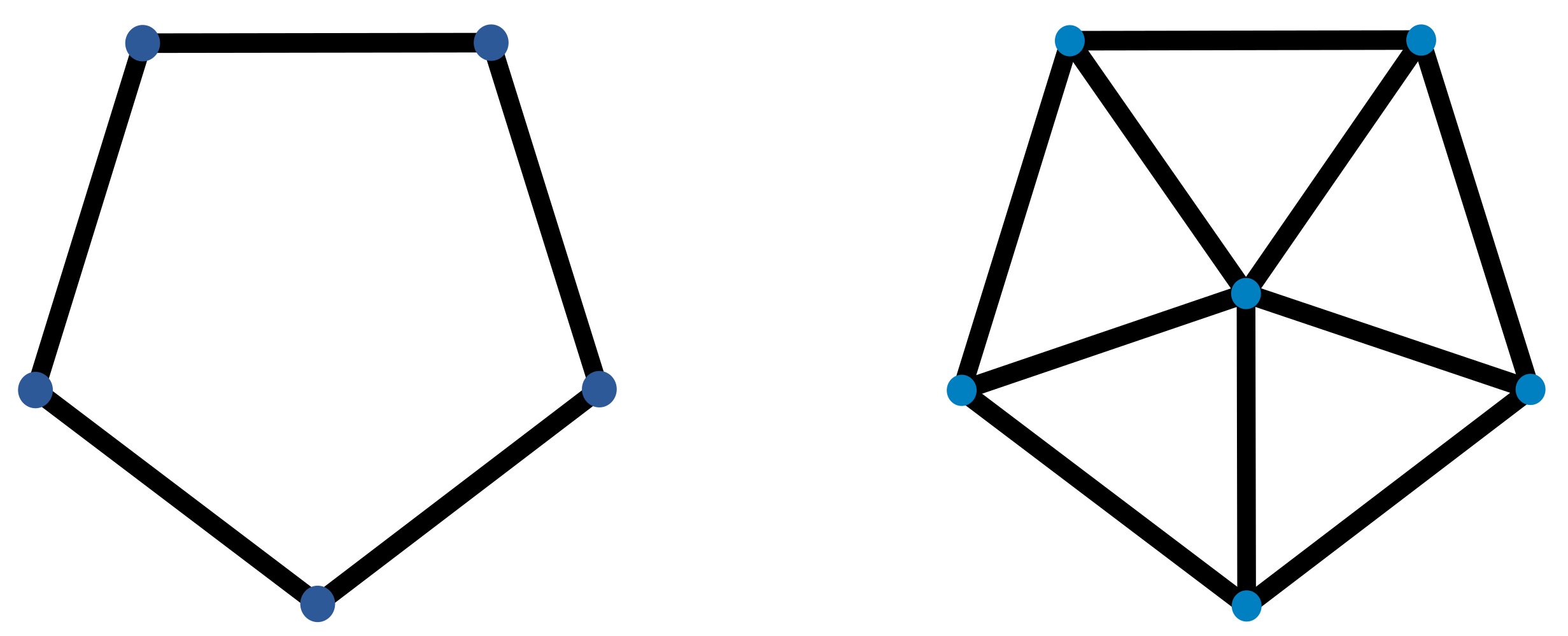While, for any $n\ge 3$, the wheel graph $W_{1+n}$ is semi-freely p-periodic, whenever p divides n, with fixed subgraph the vertex of degree n. Examples of a freely five-periodic graph and a semi-freely five-periodic graph are given in Figure 1.

Given a p-periodic graph G, the action of the finite cycle group on G defines a quotient graph $\overline{G}$. This quotient is obtained by identifying the vertices which belong to the same orbit to a single vertex and contracting the edges between vertices of distinct orbits to a single edge.

A proper coloring of a graph G is a labeling of its vertices using k integers subject to the condition that adjacent vertices have different colors. The chromatic polynomial $P_G\left(\lambda \right)$ is a classical invariant in graph theory, which counts the number of proper colorings of the vertices of the graph with $\lambda$ distinct colors. This extensively-studied polynomial can be recursively defined using a simple deletion–contraction formula. It is worth mentioning here that recent research work on graph colorings extends beyond the study of proper colorings. For more details, we refer the reader to [6,7] and references therein.

The Tutte polynomial ${\tau }_G(x,y)$ is an isomorphism invariant of graphs [8,9]. More precisely, it is a two-variable polynomial with integral coefficients which specializes to the chromatic and the flow polynomials. This invariant can also be defined recursively using a deletion-contraction formula. In this paper, we find it more convenient to write our results using Whitney’s rank generating polynomial $T_G(x,y)$, which is a modified version of the Tutte polynomial. The two invariants are related by the formula $T_G(x,y)={\tau }_G(x+1,y+1)$.

The importance of the Tutte polynomial comes not only from the large amount of information it carries about the graph, but also from its connection to other research fields such as knot theory and statistical physics. Indeed, the Jones and HOMFLY-PT polynomials of alternating links can be computed by using the Tutte polynomials of the Tait graphs associated with link diagrams [10,11]. On the other hand, the Tutte polynomial specializes to the partition function of the q-state Potts model [12].

The Tutte polynomial has been generalized into several directions. For instance, Negami [13] introduced a three-variable polynomial $N_G(u,x,y)$ which specializes to the Tutte polynomial. Another interesting generalization has been obtained by Murasugi [5] who defined a polynomial invariant of weighted graphs. Bollobas and Riordan [14] introduced a kind of universal Tutte polynomial of colored graphs with respect to the deletion-contraction formula. Another important extension has been obtained recently by Awan and Bernardi [15] who defined a version of Tutte polynomial for directed graphs. More precisely, they introduced a three-variable polynomial of digraphs $B(q,y,z)$ that specializes to the Tutte polynomial once we restrict to the underlying graphs obtained by ignoring the orientations.

The Tutte polynomial of p-periodic graphs has been studied in [16] where it was proved that this polynomial clearly reflects the periodicity of the graph as, after a suitable variable change, certain coefficients of this two-variable polynomial are null modulo p. In a more recent paper [17], we studied the behavior of the characteristic polynomial of freely periodic graphs and proved that this polynomial, with coefficients reduced modulo p, satisfies a certain congruence relation. This result has also been extended to other graph polynomials and applied as obstruction criteria to prove that certain graphs are not freely periodic with prime periods. The purpose of this paper is to investigate the behavior of the Tutte polynomial of semi-freely periodic graphs. It is noteworthy that the main motivation for this research is the nice way the coefficients of the HOMFLY-PT polynomial interact with knot symmetries, see [18,19,20] for instance. Similar results about the Yamada polynomial of symmetric spatial graphs can be found in [21]. Recall that the connection between the Tutte polynomial and knot polynomials has been established in [10,11].

This paper is organized as follows. In Section 2, we state our main results and illustrate that by some examples. In Section 3, we define the Tutte polynomial and overview some of its properties. The proofs of our results are given in Section 4. In Section 5, we discuss similar research works on graph symmetry and their extension to symmetry of knots and spatial graphs. Another example that illustrates our results is given in the Appendix A.

2. Results and Applications

In this section, we state our main results and give some examples. Indeed, we shall use Whitney’s rank generating polynomial $T_G(x,y)$ to introduce necessary conditions for a graph to be semi-freely p-periodic, for p prime. These conditions can be seen as obstructions for semi-free periodicity of graphs.

Theorem 1.

Let p be a prime and G be a semi-freely p-periodic connected graph with fixed subgraph F. Let ${\displaystyle T_G(x,y)=\sum _{i\ge 0}{P}_i\left(x\right)y^i}$, where ${\displaystyle P_i\left(x\right)=\sum _{k\ge 0}{a}_{i,k}{x}^k}$. Assume that $\left|V\right(F\left)\right|<p$, then

(a) 

For all $0\le i<p$, we have $a_{i,k}\cong 0$ modulo p, whenever $\left|V\right(F\left)\right|+np+i\le k<(n+1)p$.

(b) 

For the coefficients of the polynomial $P_0\left(x\right)$, there exist integers ${\lambda }_s$ such that $a_{0,k+sp}\cong {\lambda }_s{a}_{0,k}$ modulo p, for all $0\le k<p$.

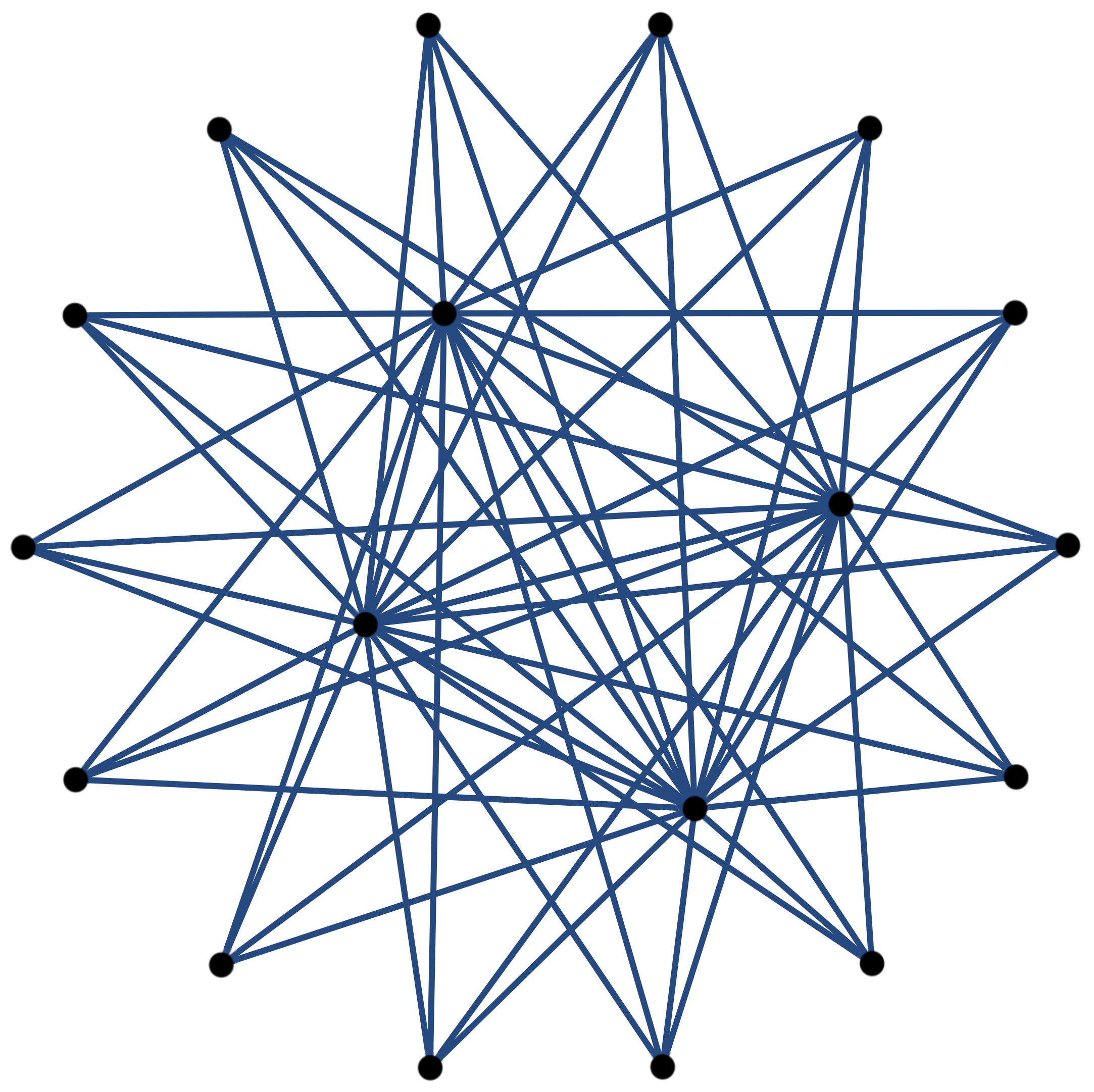
Example 1.

We shall now illustrate Theorem 1 by considering the Tutte polynomial of the complete 4-partite graph $G=K_{1,1,2,14}$, see Figure 2. This graph is semi-freely 7-periodic with the complete 3-partite graph $K_{1,1,2}$ as fixed subgraph.

Let $\overline{T_G(x,y)}$ denotes the Tutte polynomial of G with coefficients reduced modulo 7, then we have:

$$\begin{array}{cc}\hfill \overline{T_G(x,y)}\cong & 2+6x+3x^2+2x^3+x^7+3x^8+5x^9+x^{10}+x^{14}+3x^{15}+5x^{16}+x^{17}\hfill \\ & +(3+4x+5x^7+2x^8+5x^{14}+2x^{15})y+(2+x^7+x^{14})y^2\hfill \\ & +(4+4x+6x^2+x^7+x^8+5x^9)y^6+(5+5x^2+3x^7+3x^9)y^7\hfill \\ & +(2+6x+4x^7+5x^8)y^8+(6+5x^7)y^9+(6+6x+6x^7+x^8)y^{12}\hfill \\ & +(4+6x^2+x^7+6x^8)y^{13}+(2+4x+5x^2+6x^7+2x^8)y^{14}\hfill \\ & +(4+6x+5x^7+4x^8)y^{15}+(5+x^7)y^{16}+(4+2x^7)y^{18}\hfill \\ & +(3+3x+3x^7)y^{19}+(1+4x+6x^7)y^{20}+(2+6x+6x^7)y^{21}\hfill \\ & +(5x+3x^7)y^{22}+2x^7{y}^{23}+3y^{25}+(4+4x)y^{26}+(6+3x)y^{27}+(5+x)y^{28}\hfill \\ & +2x{y}^{29}+y^{32}+5y^{33}+3y^{34}+3y^{35}+5y^{36}+y^{37}+y^{39}+5y^{40}+3y^{41}\hfill \\ & +3y^{42}+5y^{43}+y^{44}.\hfill \end{array}$$

Notice that in this example we have $V\left(F\right)=4$ and the polynomial $P_0\left(x\right)$ with coefficients reduced modulo 7 is given by:

$$\overline{P_0\left(x\right)}\cong 2+6x+3x^2+2x^3+x^7+3x^8+5x^9+x^{10}+x^{14}+3x^{15}+5x^{16}+x^{17}.$$

It is clear that $P_0\left(x\right)$ satisfies condition (a) of Theorem 1. Indeed, we have $a_{0,k}\cong 0$ modulo p for $4\le k<7$ and $11\le k<14$.

Condition (b) of Theorem 1 is also satisfied. Actually, it is clear that $a_{0,k+7}\cong 4a_{0,k}$ and $a_{0,k+14}\cong 4a_{0,k}$ modulo 7, for any $0\le k<7$. In other words, we have ${\lambda }_1\cong {\lambda }_2\cong 4$ modulo 7.

Theorem 2.

Let p be a prime and G be a semi-freely p-periodic connected graph with fixed subgraph F. Let ${\displaystyle T_G(x,y)=\sum _{i\ge 0}{Q}_i\left(y\right)x^i}$, where ${\displaystyle Q_i\left(y\right)=\sum _{k\ge 0}{b}_{i,k}{y}^k}$. Assume that $\left|E\right(F\left)\right|<p$, then $b_{i,k}\cong 0$ modulo p, whenever k is not congruent to $r-\left|V\right(G\left)\right|+i+1$ modulo p, where $0\le r\le \left|E\right(F\left)\right|$.

Example 2.

We shall show that the condition given by Theorem 2 holds for the complete 4-partite graph $G=K_{1,1,2,14}$. Let us first examine the condition given by Theorem 2 for the polynomial $Q_0\left(y\right)$. Let $\overline{Q_i\left(y\right)}$ denotes the polynomial $Q_i\left(y\right)$ with coefficients reduced modulo 7. We have:

$$\begin{array}{cc}\overline{Q_0\left(y\right)}\cong \hfill & 2+3y+2y^2+4y^6+5y^7+2y^8+6y^9+6y^{12}+4y^{13}+2y^{14}+4y^{15}+5y^{16}\hfill \\ & +4y^{18}+3y^{19}+y^{20}+2y^{21}+3y^{25}+4y^{26}+6y^{27}+5y^{28}+y^{32}+5y^{33}\hfill \\ & +3y^{34}+3y^{35}+5y^{36}+y^{37}+y^{39}+5y^{40}+3y^{41}+3y^{42}+5y^{43}+y^{44}.\hfill \end{array}$$

For the graph G, we have $E\left(F\right)=5$ and $V\left(G\right)=18$. The values taken by $r-\left|V\right(G\left)\right|+1$ modulo 7, where $0\le r\le \left|E\right(F\left)\right|$ are $0,1,2,4,5,6$. Hence

$$b_{0,3}\cong b_{0,10}\cong b_{0,17}\cong b_{0,24}\cong b_{0,31}\cong b_{0,38}\cong 0, modulo 7,$$

as one can observe from the formula above. For the polynomial $\overline{Q_1\left(y\right)}$, we have

$$b_{1,4}\cong b_{1,11}\cong b_{1,18}\cong b_{1,25}\cong 0, modulo 7.$$

One may check easily that the condition given by Theorem 2 holds for $\overline{Q_i\left(y\right)}$, for any i.

It is worth mentioning that Theorems 1 and 2 hold also in the case of freely p-periodic graphs. The necessary conditions write in the same way by taking F to be the empty graph, hence $\left|V\right(F\left)\right|=\left|E\right(F\left)\right|=0$. More precisely, we have:

Corollary 1.

Let p be a prime and G be a freely p-periodic connected graph. Let ${\displaystyle T_G(x,y)=\sum _{i\ge 0}{P}_i\left(x\right)y^i}$, where ${\displaystyle P_i\left(x\right)=\sum _{k\ge 0}{a}_{i,k}{x}^k}$. Then, for all $0\le i<p$, we have $a_{i,k}\cong 0$ modulo p, whenever $i+np\le k<(n+1)p-1$.

Corollary 2.

Let p be a prime and G be a freely p-periodic connected graph. Let ${\displaystyle T_G(x,y)=\sum _{i\ge 0}{Q}_i\left(y\right)x^i}$, where ${\displaystyle Q_i\left(y\right)=\sum _{k\ge 0}{b}_{i,k}{y}^k}$. Then, $b_{i,k}\cong 0$ modulo p, whenever k is not congruent to $1+i$ modulo p.

Remark 1.

The conditions given by Theorems 1 and 2 can be better checked if the Tutte polynomial is displayed in matrix-form as explained in the Appendix A.

3. The Tutte Polynomial

This section is devoted to introduce the Tutte polynomial and briefly review some of its properties relevant to our context. More details can be found in [8,9]. The most simple way to define the Tutte polynomial is the following recursive way based on a deletion–contraction formula. Let G be a graph and e one of its edges. We denote by $G-e$ the graph obtained from G by deleting edge e and by $G/e$ we denote the graph obtained from G by deleting e and identifying the two endpoints of e. Let $E_n$ be the graph with n vertices and no edges. The Tutte polynomial is uniquely determined by the following relations

$${\tau }_G(x,y)=\left\{\begin{array}{cccc}x{\tau }_{G/e}(x,y)\hfill & & & \mathrm{if} e \mathrm{is} \mathrm{a} \mathrm{bridge}\hfill \\ y{\tau }_{G-e}(x,y)\hfill & & & \mathrm{if} e \mathrm{is} \mathrm{a} \mathrm{loop}\hfill \\ {\tau }_{G-e}(x,y)+{\tau }_{G/e}(x,y)\hfill & & & \mathrm{if} e \mathrm{is} \mathrm{an} \mathrm{ordinary} \mathrm{edge}\hfill \end{array}\right.$$

and the initialization ${\tau }_{E_n}(x,y)=1$.

Given a graph G with vertex set $V\left(G\right)$, edge set $E\left(G\right)$ and $C\left(G\right)$ connected components. Other than the recursive definition above, the Tutte polynomial can be also defined using the following subgraph expansion formula:

$${\displaystyle {\tau }_G(x,y)=\sum _{S\subseteq E\left(G\right)}{(x-1)}^{C\left(S\right)-C\left(G\right)}{(y-1)}^{\left|S\right|-\left|V\right(G\left)\right|+C\left(S\right)},}$$

where the summation is through all subsets S of $E\left(G\right)$. Note that $C\left(S\right)$ denotes the number of connected components of the subgraph of G whose edge set is S and vertex set is $V\left(G\right)$, and $\left|S\right|$ denotes the number of edges in S.

4. Proofs

In this section, we shall prove Theorems 1 and 2. Our main tool in these proofs is the subgraph expansion formula of the Tutte polynomial introduced in the previous section. Notice that for a connected graph G, the expansion formula for Whitney’s rank polynomial writes as follows:

$${\displaystyle T_G(x,y)=\sum _{S\subseteq E\left(G\right)}{x}^{C\left(S\right)-1}{y}^{\left|S\right|-\left|V\right(G\left)\right|+C\left(S\right)}.}$$

To prove Theorem 1 (a), we will start by settling the case $i=0$, the general case will be conducted similarly. Observe that the polynomial $P_0\left(x\right)$ corresponds to the contribution of the monomials $x^{C\left(S\right)-1}$ where $\left|S\right|-\left|V\right(G\left)\right|+C\left(S\right)=0$. The condition $\left|S\right|-\left|V\right(G\left)\right|+C\left(S\right)=0$ implies that S is indeed a spanning forest of the graph G,

$${\displaystyle P_0\left(x\right)=\sum _{S: \mathrm{spanning} \mathrm{forest} \mathrm{of} \mathrm{G}}{x}^{C\left(S\right)-1}.}$$

Note that the action of the cyclic group on G defines an action on the set of spanning forests of G. Since p is prime, then orbits under this action are made up of either 1 or p elements. If the orbit of a spanning forest is made up of p elements, then the contributions of the elements of this orbit to the polynomial $P_0\left(x\right)$ add to zero modulo p. Consequently, only spanning forests which are fixed by the action are to be considered in our computation of $P_0\left(x\right)$ modulo p. On the other hand, it can be easily seen that no tree can be fixed by the action unless it has a fixed vertex, hence it is adjacent to the fixed subgraph F. We conclude then that the number of trees in the spanning forest is of the from $C\left(S\right)=C\left(F^{\prime }\right)+rp$, where $F^{\prime }$ is a subgraph of F. Finally, since we assumed that $\left|V\right(F\left)\right|<p$, the coefficient of the monomial $x^k$ is zero modulo p whenever $\left|V\right(F\left)\right|+np\le k<(n+1)p-1$. Since F is nonempty, it can be easily seen that the coefficient of the monomial $x^{(n+1)p-1}$ is also congruent to zero modulo p.

The proof for the other $P_i\left(x\right)$ uses a similar argument. Note that the subgraphs that contribute to the value of $P_i\left(x\right)$ are those satisfying the condition $\left|S\right|-\left|V\right(G\left)\right|+C\left(S\right)=i$. Obviously, such a subgraph S has exactly i cycles. Again, only subgraphs S which are invariant by the action will be considered as the contribution of the other subgraphs will add to zero modulo p. Assume that S is an invariant subgraph of G that has i cycles. Then the action of the finite cyclic group on the components of S, either leaves a component fixed or the orbit of the component is made up of p elements. The assumption that the number of cycles is $i<p$ implies that each cycle is fixed under the action. Let n be the number of orbits made up each of p elements. Then $C\left(S\right)-1\le np+\left|V\right(F\left)\right|+i-1$. We conclude then that the coefficient of the monomial $x^k$ is congruent to zero modulo p whenever $\left|V\right(F\left)\right|+np+i\le k<(n+1)p$. This ends the proof of the first statement of Theorem 1.

Now, let us prove Theorem 1 (b). Recall that the coefficient $a_{0,0}$ counts the number of spanning trees which are invariant under the cyclic action, while $a_{0,p}$ counts the number of invariant spanning forests having $(p+1)$ components. Obviously, in this case one tree is fixed, while the other p trees are permuted cyclically by the action. Assume that $a_{0,p}\cong {\lambda }_1{a}_{0,0}$ modulo p for a certain integer ${\lambda }_1$. The coefficient $a_{0,1}$ is the number of spanning forests of G made up of two components each of which fixed by the action. Such spanning forest is obtained from a fixed spanning tree by removing an edge. Similarly, $a_{0,p+1}$ represents the number of invariant spanning forests made up of $p+2$ components. Such a forest admits two fixed trees and the other p trees are permuted cyclically by the action. Notice that this forest is obtained from a $(p+1)$-component forest by removing one edge. This implies that $a_{0,p+1}\cong {\lambda }_1{a}_{0,1}$ modulo p. By the same arguments we can prove that $a_{0,k+p}\cong {\lambda }_1{a}_{0,k}$ modulo p and in general $a_{0,ks+p}\cong {\lambda }_s{a}_{0,k}$ modulo p, for all $0\le k<p$. This ends the proof of Theorem 1 (b).

The proof of Theorem 2 is also based on the analysis of the subgraph expansion formula. Notice that $Q_i\left(y\right)$ is actually the sum of all monomials coming from the contribution of subgraphs S such that $C\left(S\right)-1=i$. More precisely ${\displaystyle Q_i\left(y\right)=\sum _{S\subseteq E\left(G\right),C\left(S\right)=1+i}{y}^{\left|S\right|-\left|V\right(G\left)\right|+i+1}}$. It is clear that the cyclic group ${\mathbb{Z}}_p$ acts on the set $\{S\subseteq E(G),C(S)=1+i\}$. Moreover, an orbit under this action is either made up of one or p elements. Only orbits made up of a single element will contribute to the summation modulo p. One can easily see that in this case $\left|S\right|$ is congruent to r modulo p, where $r\le \left|E\right(F\left)\right|$. Thus, $b_{i,k}\cong 0$ modulo p, whenever k is not congruent to $r-\left|V\right(G\left)\right|+i+1$ modulo p, where $r\le \left|E\right(F\left)\right|$. This completes the proof of Theorem 2.

5. Further Discussions

The graph symmetries considered in this paper have been also studied using other types of graph polynomials. For instance, Wang [22] studied the characteristic polynomial of semi-freely periodic graphs and proved that such a polynomial factorizes into a product of a polynomial associated with the fixed subgraph F and a polynomial associated with the free part of the action $G\backslash F$. Feng, Kwak, and Lee proved a formula for the characteristic polynomials of graph coverings [23]. These results have been extended to the Laplacian characteristic polynomial in [24]. A similar study of the characteristic polynomial of symmetric graphs using block circulant matrices can be found in [25]. It is worth mentioning here that most of the formulas introduced in the above mentioned papers express the polynomial of the symmetric graph G in terms of the polynomial of its quotient graph $\overline{G}$.

The advantage of the conditions introduced in Theorems 1 and 2 is that they do not involve the quotient graph. Hence, they can be easily used as obstructions to graph periodicity. Moreover, the obstructions for graph periodicity proved in this paper can be used to study the Jones and HOMFLY-PT polynomials of periodic knots. Recall that there is a simple way to associate a planar graph with any regular knot projection [26]. Such a graph is called a Tait graph of the knot. If the knot K is alternating, then its Jones polynomial $V_K\left(t\right)$ is obtained from the Tutte polynomial of its Tait graph, associated with an alternating projection, by $V_K\left(t\right)={\tau }_G(t,1/t)$, see [10]. 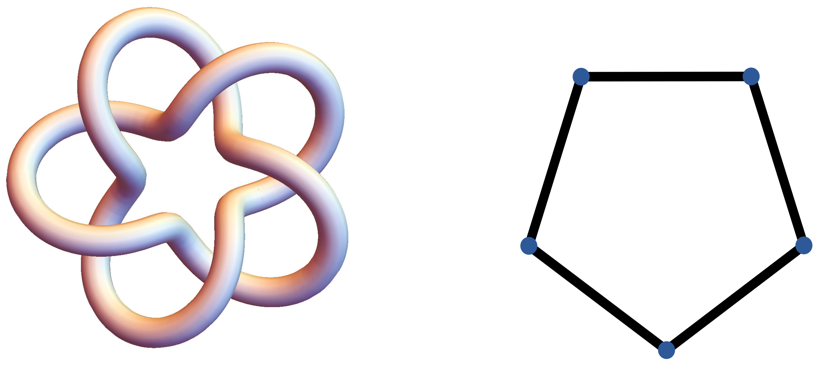A similar formula relating the Tutte polynomial and the HOMFLY-PT polynomial can be found in [11]. On the other hand, a periodic alternating knot is represented by a periodic graph, see Figure 3. A natural question that arises here is to investigate whether the conditions given by Theorems 1 and 2 extend to periodic knots. Recall that knot symmetries can be seen as a special case of the more general concept of topological symmetry groups. These groups have been introduced originally to study the symmetries of non-rigid molecules [27]. Other interesting applications of knot symmetries in the field of chemistry can be found in [28].

6. Conclusions

By using elementary properties of the Tutte polynomial, we established obstruction criteria for a graph to be symmetric. More precisely, in Theorems 1 and 2, we proved that if a given graph G is semi-freely p-periodic, then some coefficients of its Tutte polynomial, after a certain change of variables, are congruent to zero modulo p. These results have been illustrated by examples. The case of freely p-periodic graphs has been also addressed. We believe that such kind of results can be generalized to other graph polynomials. Indeed, the Negami polynomial [13] and the digraph version of Tutte polynomial [15] are both defined through subgraph expansion formulas. It seems possible to extend the methods used in this paper to study the interaction of these polynomials with graph symmetries.

References

1. Antoine, J.P. Group Theory: Mathematical Expression of Symmetry in Physics. Symmetry 2021, 13, 1354. [Google Scholar] [CrossRef]
2. Peng, F.; Yang, X.; Zhu, Y.; Wang, G. Effect of the symmetry of polyether glycols on structure-morphology-property behavior of polyurethane elastomers. Polymer 2022, 239, 124429. [Google Scholar] [CrossRef]
3. Jäntschi, L. Introducing Structural Symmetry and Asymmetry Implications in Development of Recent Pharmacy and Medicine. Symmetry 2022, 14, 1674. [Google Scholar] [CrossRef]
4. Biggs, N. Algebraic Graph Theory; Cambridge University Press: Cambridge, UK, 1993. [Google Scholar]
5. Murasugi, K. On invariants of graphs with applications to knot theory. Trans. Amer. Math. Soc. 1987, 299, 601–622. [Google Scholar]
6. Formanowicz, P.; Tanaś, K. A survey of graph coloring—Its types, methods and applications. Found. Comput. Decis. Sci. 2012, 37, 223–238. [Google Scholar] [CrossRef] [Green Version]
7. Tomescu, M.A.; Jäntschi, L.; Rotaru, D.I. Figures of Graph Partitioning by Counting, Sequence and Layer Matrices. Mathematics 2021, 9, 1419. [Google Scholar] [CrossRef]
8. Tutte, W.T. A contribution to the theory of chromatic polynomials. Can. J. Math. 1954, 6, 80–91. [Google Scholar] [CrossRef]
9. Welsh, D.J.A. The Tutte polynomial, Statistical physics methods in discrete probability, combinatorics, and theoretical computer science (Princeton, NJ, 1997). Random Struct. Algorithms 1999, 15, 210–228. [Google Scholar] [CrossRef]
10. Thistlethwaite, M.B. A spanning tree expansion of the Jones polynomial. Topology 1987, 26, 297–309. [Google Scholar] [CrossRef] [Green Version]
11. Jaeger, F. Tutte polynomials and link polynomials. Proc. American Math. Soc. 1988, 103, 647–654. [Google Scholar] [CrossRef]
12. Welsh, D.J.A. Merino, C. The Potts model and the Tutte polynomial. J. Math. Phys. 2000, 41, 1127–1152. [Google Scholar] [CrossRef]
13. Negami, S. Polynomial invariants of graphs. Trans. Amer. Math. Soc. 1989, 314, 1–49. [Google Scholar]
14. Bollobas, B.; Riordan, O. A Tutte Polynomial for Coloured Graphs. Comb. Probab. Comput. 1999, 8, 45–93. [Google Scholar] [CrossRef]
15. Awan, J.; Bernardi, O. Tutte polynomials for directed graphs. J. Comb. Theory B 2020, 140, 192–247. [Google Scholar] [CrossRef]
16. Chbili, N. A note on the Tutte polynomial and automorphism group of a graph. Asian Eur. J. Math. 2014, 7, 1450001. [Google Scholar] [CrossRef]
17. Chbili, N. Graph Polynomials and Symmetries. J. Algebra Its Appl. 2019, 1950172. [Google Scholar] [CrossRef] [Green Version]
18. Traczyk, P. A criterion for knots of period 3. Topol. Its Appl. 1990, 36, 275–281. [Google Scholar] [CrossRef] [Green Version]
19. Traczyk, P. Periodic knots and the skein polynomial. Invent. Math 1991, 106, 73–84. [Google Scholar] [CrossRef]
20. Chbili, N. The skein polynomial of freely periodic knots. Topol. Appl. 2002, 121, 535–542. [Google Scholar] [CrossRef] [Green Version]
21. Chbili, N. Skein algebras of the solid torus and symmetric spatial graphs. Fund. Math. 2006, 190, 1–10. [Google Scholar] [CrossRef] [Green Version]
22. Wang, K. Characteristic polynomials of symmetric graphs. Linear Algebra Its Appl. 1983, 51, 121–125. [Google Scholar] [CrossRef] [Green Version]
23. Feng, R.; Kwak, J.H.; Lee, J. Characteristic polynomials of graph coverings. Bull. Austral. Math. Soc. 2004, 69, 133–136. [Google Scholar] [CrossRef]
24. Li, D.; Hou, Y. Laplacian of a Graph Covering and Its Applications. Bull. Malays. Math. Sci. Soc. 2019, 42, 2569–2583. [Google Scholar] [CrossRef]
25. Chbili, N.; Al Dhaheri, S.; Tahnon, M.Y.; Abunamous, A.A.E. The Characteristic Polynomials of Symmetric Graphs. Symmetry 2018, 10, 582. [Google Scholar] [CrossRef] [Green Version]
26. Adams, C. The Knot Book: An Elementary Introduction to the Mathematical Theory of Knots; American Mathematical Society: Providence, RI, USA, 1994. [Google Scholar]
27. Flapan, E.; Lawrence, E.D.; Wilson, R.D. Topological Symmetry Groups of the Heawood Graph. Symmetry 2020, 12, 546. [Google Scholar] [CrossRef]
28. Yuzhong, L.; O’keeffe, M.; Treacy, M.M.J.; Yaghi, O.M. The geometry of periodic knots, polycatenanes and weaving from a chemical perspective: A library for reticular chemistry. Chem. Soc. Rev. 2018, 47, 4642–4664. [Google Scholar]
Figure 1. A freely 5-periodic graph (left) and a semi-freely 5-periodic graph (right).
Symmetry 14 02072 g001
Figure 2. The complete 4-partite graph K 1 , 1 , 2 , 14 is semi-freely 7-periodic.
Symmetry 14 02072 g002
Figure 3. A 5-periodic knot (left) and its associated 5-periodic Tait graph (right).
Symmetry 14 02072 g003
Publisher’s Note: MDPI stays neutral with regard to jurisdictional claims in published maps and institutional affiliations.