Abstract
We focus on a variety of bivariate models with proportional hazard components. Models with proportional hazard marginals are described together with a selection of models with proportional hazard conditional distributions. The bivariate distributions with marginal proportional hazards distributions are shown to be closely related to certain known bivariate exponential models. Two distinct kinds of conditional specification are investigated. Discussion is provided of cases with hazard function components that are (1) completely unknown, (2) known to belong to given parametric families and (3) completely known. Since the models are designed for use with survival data, it is inevitable that the marginal and conditional distributions will be asymmetric. However, logarithmic transformations in some cases will result in symmetric component distributions.
1. Introduction
Survival models involving families of densities with proportional hazard functions have proved to be useful for analyzing many lifetime data sets. Not infrequently bivariate survival data (involving related lifetimes) need to be analyzed. In this paper, we review several methods for generating suitable bivariate models for such situations. The key observation in the development is that proportional hazard models can be viewed as ones obtained via monotone transformations applied to exponential models. In the latter sections of the paper, related statistical inference issues are discussed. Since the models are designed for use with survival data, it is inevitable that the marginal and conditional distributions will be asymmetric. However, logarithmic transformations in some cases will result in symmetric component distributions.
2. Bivariate Distributions with Proportional Hazard Marginals
Let and be two absolutely continuous distribution functions with support and with corresponding densities and and hazard functions and (where ).
We will say that has a bivariate marginal proportional hazard distribution associated with and and with parameters if for
and we will write and also (here is an acronym for proportional hazard marginals). Note that the name is appropriate since for
Observe that if then the ’s admit a representation of the form
where for each i, (i.e., ).
Note that the transformations in (3) are monotone increasing.
In fact, it is not necessary to build the model with reference to two distribution functions and Instead we can begin with and use two monotone increasing functions to define If we denote the corresponding inverse functions by then it is readily verified that each has a proportional hazard distribution, i.e., that for
It is however customary to use the representation (3) involving the two distribution functions and and we will adhere to this convention.
Of course, in the representation (3), can have any bivariate exponential distribution that we wish to utilize. Popular choices of bivariate exponential distributions involving few additional parameters include:
- (i)
- Gumbel Type I distribution, with
- (ii)
- Gumbel Type II distribution, with
- (iii)
- Marshall–Olkin distribution (see Marshall and Olkin [1]), with
Many other choices are possible, see for example Kotz et al. ([2], pp. 350–385).
For a specific example, if we choose to have a Gumbel Type I density, i.e.,
and use and then the resulting PHM density will be of the form:
In application of such models, it is frequently desirable to postulate that each is a member of some parametric family of distributions to add flexibility to the model. The dependence structure will however be completely determined by the copula of the particular bivariate exponential distribution used in the construction.
Alternatively, one could “let the data tell us which ’s to use in the model”. Thus, we would seek monotone marginal transformations that will make the transformed marginal sample distributions look as much like exponential distributions as possible. This semi-parametric approach will be returned to later in the paper.
3. Bivariate Distributions with Proportional Hazard Conditionals
We will consider two types of conditioning. The first kind is quite traditional in that we consider the distribution of one variable given that a second variable takes on a particular value. The second kind involves conditioning on the event that the second variable is larger than a particular value.
3.1. The First Kind
Consider two proportional hazard families of densities as in (1). Recall that we write if the corresponding densities are given by (1).
For this conditional proportional hazards paradigm, we seek to identify joint distributions for with all conditional densities of the forms in (1). Thus, for each we wish to have
and for each
for some functions and It is not difficult to verify that this will be the case if and only if
where has a joint distribution with exponential conditionals, i.e., such that for each
and for each
The class of all densities with such exponential conditionals is identified in Arnold and Strauss [3] and is of the form:
where and The normalizing constant, in (10) can be expressed in terms of the exponential integral function. Thus
Consequently, bivariate densities with conditionals of the proportional hazard form will be given by
This model is discussed in Arnold and Kim [4] and we will follow their nomenclature and call it a proportional hazard conditionals model of the first kind. If has a density of the form (13), we will write
3.2. The Second Kind
Again consider two proportional hazard families of densities as in (1). Recall that we write if the corresponding densities are given by (1). The second kind of conditional model (also introduced in Arnold and Kim [4]) involves conditioning on events of the form and Thus, we seek to identify joint survival functions for such that for each
and for each
for some functions and
To analyze this situation (since and are known) it is again convenient to write
where the ’s are exponential random variables.
The conditions (14) and (15) are then equivalent to the statements
and
Denote the survival functions of and by and It then follows that
Taking logarithms we have:
This is a Stephanos–Levi–Civita–Suto functional Equation (see Arnold et al. [5], p. 13) which is readily solved to yield the following expression for the joint survival function of
for where and This is recognizable as Gumbel’s Type I bivariate exponential distribution (with exponential marginals). From Equation (21) we obtain the joint survival function of in the form:
Then, the joint cumulative distribution function is
and the joint density function is
The vector with density (21) has exponential marginals, i.e., for and thus for Consequently, for the conditional densities are given by
If has a survival function of the form (22), we write
note that and in (22) will be independent if and only if
4. If and Are Known
Suppose that we have available a sample of size from one of the bivariate proportional hazard models discussed in this paper. Since and are known, it is appropriate to transform the data to obtain
and thus to have a sample from the corresponding well-known bivariate exponential distribution. See the following references for appropriate estimation strategies for these bivariate exponential data sets:
- Gumbel [6],
- Besag [7],
- Arnold and Strauss ([3,8]),
- Castillo and Hadi [9],
- Arnold et al. [5].
5. If and Are Known to Belong to Some Given Parametric Families
We will illustrate this with a particular example. Other examples may treated in analogous fashion. Suppose that in the PHC(II) model, (23), we replace by and by where the parameters and are unknown. In this case, the model becomes more complicated, but we can still envision success in estimating all the parameters in the model. As a specific example, consider the following distributions of the Weibull form:
and
The corresponding log-likelihood function is of the form
The score function , has elements which are derivative of the log-likelihood function with respect to the parameters and thus are given by
By equating the scores to zero we obtain the score equations, i.e., (). These equations are typically solved by means of Newton–Raphson or quasi-Newton numerical methods to obtain the maximum likelihood estimators of the parameter vector . The observed information matrix of is given by , i.e., with elements of the form of minus the second derivative of the log-likelihood function with respect to the parameters. The Fisher information matrix of vector is given by and should be calculated numerically.
When, we use the base distributions (26) and (27) in the model, a technique known as pseudo-likelihood estimation (see Arnold and Strauss [10]) will provide estimates of all five parameters in the model. Besag [7], defined the pseudo-likelihood estimator of as the value of that maximizes the pseudo likelihood function, which in the present bivariate situation is based on the conditional PH densities and is given by
Thus for the example with distributions:
and
we have the following log pseudo likelihood.
Parallel to the definition of the score function, the pseudo−score function is defined to be the vector whose coordinates are partial derivatives of the log-pseudo-likelihood function with respect to each of the parameters in the model. It is denoted by
The estimating equations are constructed by setting the elements of the pseudo−score vector equal to zero. Solutions of these equations correspond to the pseudo-likelihood estimates of the parameters of the model. Typically, these solutions are obtained numerically using iterative methods such as Newton–Raphson or quasi-Newton.
The pseudo-likelihood estimator of obtained in the above fashion can be verified to be consistent and asymptotically normally distributed with covariance matrix given by
(see Arnold and Strauss [10]), where for
As a consistent estimate of the asymptotic variance-covariance matrix of the pseudo-likelihood estimator, we will use the sandwich estimator proposed by Cheng and Riu [11]. This estimator is developed as follows.
Let be the vector of pseudo-scores for the i-th observation. Then define
which is the sum over all the observations of the matrices of second derivatives of evaluated at the pseudo-likelihood estimator In addition, define
Using this, we construct a consistent sandwich estimator of the asymptotic variance-covariance matrix in the form
A detailed discussion and analysis of such a model, but with power Lindley base distributions, utilizing pseudo-likelihood estimation, may be found in Martínez-Flórez et al. [12].
6. If and Are Unknown
All but one of the bivariate proportional hazard models described in this paper have marginals of the proportional hazard form. The exception is the PHC(I) model which, for unknown and , we will discuss in Section 7. For the other models, we know that if and were known, we could transform the data to obtain a sample from a well-known bivariate exponential model. Consequently, if we consider an estimate of based on and an estimate of based on , we can transform the data using
and
and then we will have approximately a sample from a bivariate distribution with standard exponential marginals and we can then estimate the parameters in this exponential model. Note that for identifiability in unknown and models we have to fix and to be equal to
For the PHC(II) model with Weibull component distributions, given in (26) and (27), a small simulation study of the performance of the maximum likelihood parameter estimates has been implemented for a variety of sample sizes and for several parametric configurations. With minimal loss of generality we set throughout the simulation study. Three values of the dependence parameter were used, namely and , together with four sample sizes . The table presents results for three representative choices of values for and . As for measures of performance, the relative bias (RB) and the square root of the mean squared error (MSE) are given.
The results in Table 1 confirm that both the relative bias and the root mean-squared error of the estimates decrease as sample size increases.

Table 1.
RB and for the PHC(II)-Weibull model.
7. If and Are Unknown in the PHC(I) Model
Our model is of the form, i.e.,
where and are unknown. Although it would be easy to estimate , via pseudolikelihood, if and were known, it is not apparent how to estimate and assuming that is known. So it is not clear how to implement an iterative strategy for estimating , and simultaneously. Perhaps our only choice is to assume that the ’s belong to some parametric families of distributions, with once more utilizing pseudo likelihood to avoid dealing with
8. Application
The data analyzed in this example consist of the maximum water levels registered at two stations on the Fox river in Wisconsin during the period 1918–1950. Measurements were made at an upstream location (Berlin, ) and a downstream location (Wrightstown, ). This data set was previously analyzed by Gumbel and Mustafi [13] using a bivariate extreme model.
In our analysis of this data set we will fit four models namely:
- The Arnold and Strauss [3] bivariate exponential conditionals distribution. denoted by BEC.
- Gumbel’s [6] first bivariate exponential distribution, denoted by BG(I).
- The proportional hazard conditionals Weibull extension of the BEC distribution, denoted by PHC(I)-W.
- The proportional hazard conditionals Weibull extension of the BG(I) distribution, denoted by PHC(II)-W.
In both of the Weibull proportional hazard conditionals extensions mentioned above, i.e., PHC(I)-W and PHC(II)-W, as described in Section 3, we use the following choices for the component distributions and :
and
Using the Arnold and Strauss [3] density given in Equation (11), the density of the PHC(I)-W is given by
The corresponding log-pseudo-likelihood function for a sample of size n takes the form
The log-pseudo-likelihood for the BEC model is obtained from the expression for the PHC(I)-W by setting and .
The log-likelihood function for a sample of size n from the PHC(II)-W is of the form given in Equation (28), with simple change of notation. In this case the corresponding log-likelihood function for the BG(I) model is again obtained by setting and .
Using the Fox river data, maximizing the log-likelihood for the models BG(I) and PHC(II)-W and the log-pseudo-likelihood for the models BEC and PHC(I)-W, we obtain the estimates of the parameters of the four models given in Table 2 (with standard errors in parentheses).
Table 2.
Estimates (standard errors) for the fitted models.
To compare model fitting, we use the AIC (Akaike [14]) criterion, namely AIC = We also consider the BIC (Schwarz [15]) criterion, namely BIC = criterion where p is the number of parameters for the model being considered. The best model is the one with the smallest AIC or BIC.
According to the values of the AIC and BIC criteria for the Fox river data, the best model is the PHC(I)-W followed by the PHC(II)-W model.
Since the BEC and BG(I) models are special cases of the PHC(I)-W and PHC(II)-W models, respectively, obtained by setting , we may test the hypotheses
for comparing the PHC(II)-W and PHC(I)-W models with the BG(I) and BEC models, respectively.
Using the likelihood ratio statistic,
we obtain
The corresponding values of in each case are provided in Table 3 (note in the BEC-PHC(I)-W comparison the log-pseudo-likelihoods have been utilized instead of log-likelihoods) which are greater than the value of the indicating that the PHC(II)-W and PHC(I)-W models are significantly better at the 1% level. Thus, the PHC(II)-W and PHC(I)-W models appear to be good alternative for fitting the set data. The choice between the PHC(I)-W and PHC(II)-W is not so clear-cut, but perhaps the PHC(I)-W might be considered to be marginally better.
Table 3.
Comparison of likelihood ratio statistics.
The graphs in Figure 1a,b and Figure 2a,b show the contours of the densities BG(I) and BEC and of the fitted models for PHC(II)-W and PHC(I)-W, respectively.
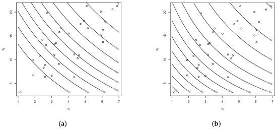
Figure 1.
Contours for (a) BG(I) model and (b) BEC model.

Figure 2.
Contours for (a) PHC(II)-W model and (b) PHC(I)-W model.
Under the assumption that the forms of the ’s are unknown, we use the transformations
to arrive at a BG(I) model with joint survival function
Then, using the expression for the maximum likelihood estimate of provided by Kotz et al. ([2], p. 352), we obtain a much smaller value than the estimated value of the parameter obtained assuming a known form for the ’s. Perhaps this indicates that the Weibull choices for the ’s are not optimal.
9. Discussion
The bivariate models discussed in this paper utilize quite different approaches to their construction and thus can be expected to exhibit significantly different distributional properties, especially with regard to dependence. Future research on such models should put some focus on the problem of selecting the appropriate one of these models for a particular data set. Of course, the old stand-by of fitting via maximum likelihood and comparing models via AIC and BIC is always available.
Author Contributions
Conceptualization, B.C.A., G.M.-F. and H.W.G.; Formal analysis, B.C.A., G.M.-F. and H.W.G.; Investigation, B.C.A., G.M.-F. and H.W.G.; Methodology, B.C.A. and G.M.-F.; Software, G.M.-F.; Supervision, B.C.A. and H.W.G.; Validation, B.C.A., G.M.-F. and H.W.G. Writing—original draft preparation, B.C.A., G.M.-F. and H.W.G.; Funding acquisition, H.W.G. All of the authors contributed significantly to this research article. All authors have read and agreed to the published version of the manuscript.
Funding
The research of H.W. Gómez was supported by SEMILLERO UA-2022 project, Chile. The research of G. Martínez-Flórez was supported by Universidad de Córdoba, Montería, Colombia.
Data Availability Statement
The data can be found in Gumbel and Mustafi (1967).
Acknowledgments
The authors thank the Editor and three anonymous referees for their constructive comments and suggestions, which have greatly helped them to improve the paper.
Conflicts of Interest
The authors declare no conflict of interest.
References
- Marshall, A.W.; Olkin, I. A Multivariate Exponential Distribution. J. Am. Statist. Assoc. 1967, 62, 30–44. [Google Scholar] [CrossRef]
- Kotz, S.; Balakrishnan, N.; Johnson, N.L. Continuous Multivariate Distributions; John Wiley and Sons: Hoboken, NJ, USA, 2000. [Google Scholar]
- Arnold, B.C.; Strauss, D.J. Bivariate distributions with exponential conditionals. J. Am. Statist. Assoc. 1988, 83, 522–527. [Google Scholar] [CrossRef]
- Arnold, B.C.; Kim, Y.H. Conditional proportional hazards models. In Lifetime Data: Models in Reliability and Survival Analysis; Jewell, N.P., Kimber, A.C., Lee, M.L.T., Whitmore, G.A., Eds.; Springer: Boston, MA, USA, 1996; pp. 21–28. [Google Scholar]
- Arnold, B.C.; Castillo, E.; Sarabia, J.M. Conditional Specification of Statistical Models; Springer Series in Statistics; Springer: Berlin/Heidelberg, Germany, 1999. [Google Scholar]
- Gumbel, E.J. Bivariate Exponential Distributions. J. Am. Statist. Assoc. 1960, 55, 698–707. [Google Scholar] [CrossRef]
- Besag, J. Statistical Analysis of Non-Lattice Data. J. R. Stat. Soc. Ser. D 1975, 24, 179–195. [Google Scholar] [CrossRef]
- Arnold, B.C.; Strauss, D.J. Bivariate distributions with conditionals in prescribed exponential families. J. R. Stat. Soc. Ser. B 1991, 53, 365–375. [Google Scholar] [CrossRef]
- Castillo, E.; Hadi, A.S. Modeling Lifetime Data with Application to Fatigue Models. J. Am. Statist. Assoc. 1995, 90, 1041–1054. [Google Scholar] [CrossRef]
- Arnold, B.C.; Strauss, D.J. Pseudolikelihood estimation: Some examples. Sankhya Ser. B 1991, 53, 233–243. [Google Scholar]
- Cheng, C.; Riu, J. On estimating linear relationships when both variables are subject to heteroscedastic measurement errors. Technometrics 2006, 48, 511–519. [Google Scholar] [CrossRef]
- Martínez-Flórez, G.; Arnold, B.C.; Gómez, H.W. A bivariate power Lindley survival distribution. 2022; Unpublished Work. [Google Scholar]
- Gumbel, E.; Mustafi, C.K. Some Analytical Properties of Bivariate Extremal Distributions. J. Am. Statist. Assoc. 1967, 62, 569–588. [Google Scholar] [CrossRef]
- Akaike, H. A new look at the statistical model identification. IEEE Trans. Autom. Control 1974, 19, 716–723. [Google Scholar] [CrossRef]
- Schwarz, G. Estimating the dimension of a model. Ann. Stat. 1978, 6, 461–464. [Google Scholar] [CrossRef]
Publisher’s Note: MDPI stays neutral with regard to jurisdictional claims in published maps and institutional affiliations. |
© 2022 by the authors. Licensee MDPI, Basel, Switzerland. This article is an open access article distributed under the terms and conditions of the Creative Commons Attribution (CC BY) license (https://creativecommons.org/licenses/by/4.0/).