Prospects for Heavy Neutral SUSY HIGGS Scalars in the hMSSM and Natural SUSY at LHC Upgrades

Abstract

We examine production and decay of heavy neutral SUSY Higgs bosons $pp\to H,A\to \tau \overline{\tau }$ within the hMSSM and compare against a perhaps more plausible natural supersymmetry scenario dubbed $m_h^{125}\left(\mathrm{nat}\right)$ which allows for a natural explanation for $m_{weak}\simeq m_{W,Z,h}\sim 100$ GeV while maintaining $m_h\simeq 125$ GeV. We evaluate signal against various Standard Model backgrounds from $\gamma ,Z\to \tau \overline{\tau }$, $t\overline{t}$ and vector boson pair production $VV$. We combine the transverse mass method for back-to-back (BtB) taus along with the ditau mass peak $m_{\tau \tau }$ method for acollinear taus as our signal channels. This technique ultimately gives a boost to the signal significance over the standard technique of using just the BtB signal channel. We evaluate both the 95% CL exclusion and $5\sigma$ discovery reach in the $m_A$ vs. $tan\beta$ plane for present LHC with 139 fb⁻¹, Run 3 with 300 fb⁻¹ and high luminosity LHC (HL-LHC) with 3000 fb⁻¹ of integrated luminosity. For $tan\beta =10$, the exclusion limits range up to $m_A\sim 1$, 1.1 and 1.4 TeV, respectively. These may be compared to the range of $m_A$ values gleaned from a statistical analysis of the string landscape wherein $m_A$ can range up to $\sim 8$ TeV.

1. Introduction

The search for R-parity conserving supersymmetric (SUSY) particles at colliding beam experiments is plagued by the necessity to pair produce sparticles, and by the fact that the sparticle cascade decay terminates in the lightest SUSY particle (LSP), usually assumed to comprise at least a portion of the missing dark matter in the universe. The first of these thus requires enough energy to produce two rather than just one sparticle, while the second of these means that the sparticle invariant mass can not be directly reconstructed as a resonance. An alternative path to SUSY discovery at collider experiments is to search for the R-parity even neutral heavy Higgs bosons, the heavy scalar H and the pseudoscalar A. These particles can be produced singly as s-channel resonances and have the advantage in that their invariant mass can, in principle, be directly reconstructed (as was the case in discovery of the light scalar h).

In this paper, we examine production and decay of the heavy neutral scalar Higgs bosons of the MSSM in the most lucrative discovery channel $pp\to H,A\to \tau \overline{\tau }$. In previous phenomenological work [1,2,3,4,5], new scenarios were proposed for the $m_A$ vs. $tan\beta$ discovery plane which ensured that $m_h\simeq 125$ GeV while also respecting that LHC sparticle search limits were enforced, usually by assuming supersymmetry breaking in the multi-TeV regime. These constraints can in principle affect the regions of the heavy Higgs search planes which can be probed by current and forthcoming hadron colliders.

In the present work, we add to these constraints the condition that the magnitude of the weak scale also be natural. This is because natural SUSY models are in a sense more plausible than unnatural models [6]. For our naturalness criterion, we adopt the notion of practical naturalness [7]:

An observable $\mathcal{O}=o_1+\cdots +o_n$ is natural if all independent contributions to $\mathcal{O}$ are comparable to or less than $\mathcal{O}$.

Here, we adopt the measured value of the Z-boson mass as representative of the magnitude of weak scale, where in the Minimal Supersymmetric Standard Model (MSSM) [8], the Z mass is related to Lagrangian parameters via the electroweak minimization condition

$$m_Z^2/2=\frac{m_{H_d}^2+{\Sigma }_d^d-(m_{H_u}^2+{\Sigma }_u^u){tan}^2\beta }{{tan}^2\beta -1}-{\mu }^2$$

(1)

where $m_{H_u}^2$ and $m_{H_d}^2$ are the Higgs soft breaking masses, $\mu$ is the (SUSY preserving) superpotential $\mu$ parameter and the ${\Sigma }_d^d$ and ${\Sigma }_u^u$ terms contain a large assortment of loop corrections (see Appendices of Refs [9,10,11] for leading two-loop corrections). For natural SUSY models, the naturalness measure [12]

$${\Delta }_{EW}\equiv |maximaltermontheright-hand-sideofEquation\left(1\right)|/(m_Z^2/2)$$

(2)

is adopted here where a value

$${\Delta }_{EW}\lesssim 30$$

(3)

fulfills the comparable condition of practical naturalness. For most SUSY benchmark models, the superpotential $\mu$ parameter is tuned to cancel against large contributions to the weak scale from SUSY breaking. Since the $\mu$ parameter typically arises from very different physics than SUSY breaking, e.g., from whatever solution to the SUSY $\mu$ problem that is assumed, (Twenty solutions to the SUSY $\mu$ problem are recently reviewed in Ref. [13].) then such a “just-so” cancellation seems highly implausible [6] (though not impossible) compared to the case where all contributions to the weak scale are $\sim m_{weak}$, so that $\mu$ (or any other parameter) need not be tuned.

There are several important implications of Equation (3) for heavy neutral SUSY Higgs searches.

• The superpotential $\mu$ parameter enters ${\Delta }_{EW}$ directly, leading to $\left|\mu \right|\lesssim 350$ GeV. This implies that for heavy Higgs searches with $m_{A,H}\gtrsim 2\left|\mu \right|$, then SUSY decay modes of $H,A$ should typically be open. If these additional decay widths to SUSY particles are large, then the branching fraction to the $\tau \overline{\tau }$ discovery mode can be substantially reduced.
• For $m_{H_d}\gg m_{H_u}$, then $m_{H_d}$ sets the heavy Higgs mass scale ($m_{A,H}\sim m_{H_d}$) while $m_{H_u}$ sets the mass scale for $m_{W,Z,h}$. Then naturalness requires [14]

$$m_{A,H}\lesssim m_{Z}tan\beta \sqrt{{\Delta }_{EW}}.$$

(4)

For $tan\beta \sim 10$ with ${\Delta }_{EW}\lesssim 30$, then $m_A$ can range up to $\sim 5$ TeV. For $tan\beta \sim 40$, then $m_A$ stays natural up to $\sim 20$ TeV (although for large $tan\beta \gtrsim 20$, then bottom squark contributions to ${\Sigma }_u^u$ become large and provide typically much stronger limits on natural SUSY spectra). Since most $H,A\to \tau \overline{\tau }$ searches and projected reach limits take place assuming a decoupled SUSY spectra, then such results can overestimate the collider heavy Higgs reach since in general the presence of $H,A\to SUSY$ decay modes will diminish the $H,A\to \tau \overline{\tau }$ branching fraction.

Using naturalness, in Section 2 we propose a new natural SUSY benchmark scenario $m_h^{125}\left(\mathrm{nat}\right)$ which is also consistent with expectations from the string landscape [15]. In Section 3, we discuss production and decay of heavy neutral Higgs bosons in the $m_h^{125}\left(\mathrm{nat}\right)$ scenario. In Section 4, we discuss signal event generation and SM backgrounds for the case of back-to-back (BtB) $\tau$s in the transverse plane using the total transverse mass variable $m_T^{tot}$. In Section 5, we discuss signal and background for the acollinear tau pairs using the $m_{\tau \tau }$ variable. Including this signal channel can lead to a substantial increase in signal significance and so combined with the BtB $\tau$s can give an increased collider reach in the $m_A$ vs. $tan\beta$ search plane. In Section 6, we present our reach of present LHC with 139 fb⁻¹ and also the projected reach of LHC Run3 and high-luminosity LHC (HL-LHC). Our conclusions reside in Section 7.

2. The Natural SUSY Higgs Search Plane

The mass of the light SUSY Higgs boson is given approximately by [16]

$$m_h^2\simeq m_Z^2{cos}^{2}2\beta +\frac{3g^2}{8{\pi }^2}\frac{m_t^4}{m_W^2}\left[ln\frac{m_{\tilde{t}}^2}{m_t^2}+\frac{x_t^2}{m_{\tilde{t}}^2}\left(1-\frac{x_t^2}{12m_{\tilde{t}}^2}\right)\right]$$

(5)

where $x_t=A_t-\mu cot\beta$ and $m_{\tilde{t}}^2\simeq m_{Q_3}{m}_{U_3}$ is the mean top squark mass. For a given value of $m_{\tilde{t}}^2$, then $m_h^2$ is maximal for $x_t^{max}=\pm \sqrt{6}{m}_{\tilde{t}}$.

2.1. Some Previous SUSY Higgs Benchmark Studies

In Ref. [1], a variety of SUSY Higgs search benchmark points were proposed, including 1. the $m_h^{max}$ scenario where a value of $x_t^{max}$ was chosen along with $m_{\tilde{g}}=1500$ GeV and $m_{SUSY}\equiv m_{\tilde{t}}=1$ TeV with $\mu =M_2=0.2$ TeV as a conservative choice which maximized the parameter space of the $m_A$ vs. $tan\beta$ plane available for new SUSY Higgs boson searches. Similarly, $m_h^{mod+}$ and $m_h^{mod-}$ scenarios were proposed with similar parameters except for more moderate $x_t=1.6m_{SUSY}$ and $x_t=-2.2m_{SUSY}$ values. Light stop, light stau, $\tau$-phobic and low $m_H$ scenarios were proposed as well. Over time, all these benchmark models have become LHC-excluded since (at least) they all proposed $m_{\tilde{g}}\sim 1500$ GeV while after LHC Run 2 the ATLAS/CMS Collaborations require $m_{\tilde{g}}\gtrsim 2.2$ TeV [17,18].

In Ref. [4], an $m_h^{125}$ benchmark model was proposed with $m_{SUSY}\sim 1.5$ TeV, $\mu =1$ TeV and $m_{\tilde{g}}=2.5$ TeV in accord with LHC Run 2 gluino mass constraints. The $x_t=2.8$ TeV value was chosen to nearly maximize the value of $m_h$ given the other parameters of the model. This model has almost all $H,A\to SUSY$ decay modes kinematically closed due to the heavy SUSY spectra so it closely resembles the type-II two-Higgs doublet model (2HDM) phenomenology [19]. An $m_h^{125}\left(\tilde{\tau }\right)$ scenario (exemplifying bino-stau coannihilation was selected with $\mu =1$ TeV along with a $m_h^{125}\left(\tilde{\chi }\right)$ scenario with $\mu =180$ GeV, $M_1=160$ GeV and $M_2=180$ GeV so that $H,A$ decay to many electroweakino states is allowed. Furthermore, an $m_h^{125}\left(align\right)$ model with specific alignment without decoupling [20,21] parameters with $\mu =7.5$ TeV was chosen along with a $m_H^{125}$ scenario where the heavy Higgs scalar was actually the 125 GeV Higgs boson. These scenarios would be hard pressed to explain why $m_{weak}\sim 100$ GeV due to the tuning needed for such large $\mu$ parameters. The exception is the $m_h^{125}\left(\tilde{\chi }\right)$ scenario, although here the peculiar gaugino/higgsino mass choices seem at odds with most theory expectations (Gaugino mass unification is usually expected in models based on grand unification, but is also expected by the simple form of the supergravity (SUGRA) gauge kinetic function which depends typically on only a single hidden sector field in many string-inspired constructs.).

A somewhat different approach is taken in the model labelled hMSSM [2,3,22]. In the hMSSM, by adopting a high $m_{SUSY}$ scale and by neglecting some small radiative corrections to the Higgs mass matrix, then one may use $m_h$ (along with $m_A$ and $tan\beta$) as an input parameter with Higgs mixing angle $\alpha$, $m_H$ and $m_{H^{\pm }}$ as outputs. This ensures that $m_h=125$ GeV is enforced throughout the remaining Higgs search parameter space. The adoption of a high value $m_{SUSY}\gtrsim 1$ TeV then makes this model look like the 2HDM, and sparticle mass spectra are effectively neglected. By combining $H,A\to \tau \overline{\tau }$ with $H,A\to t\overline{t}$ at lower $tan\beta$, then it is claimed almost the entire $m_A$ vs. $tan\beta$ parameter space can be probed by HL-LHC for $m_A\lesssim 1$ TeV [3].

2.2. Status of Run 2 LHC Searches

The ATLAS Collaboration has reported on a search for $H,A\to \tau \overline{\tau }$ at CERN LHC Run 2 using 139 fb⁻¹ of integrated luminosity at $\sqrt{s}=13$ TeV [23]. The study focusses on back-to-back $\tau \overline{\tau }$ states where transverse opening angles $\Delta \varphi \left({\tau }_{had}{\tau }_{had}\right)>{155}^{\circ }$ and $\Delta \varphi \left({\tau }_{lep}{\tau }_{had}\right)>{135}^{\circ }$ are required. Mixed leptonic-hadronic (${\tau }_{lep}{\tau }_{had}$) and hadronic-hadronic (${\tau }_{had}{\tau }_{had}$) final states are combined. The hadronic tau tagging efficiency in one or three charged prong $\tau$-jets varies from 60 to 85%. The total transverse mass [24]

$$m_T^{tot}=\sqrt{{(p_T^{{\tau }_1}+p_T^{{\tau }_2}+E_T^{miss})}^2-{({\overrightarrow{p}}_T^{{\tau }_1}+{\overrightarrow{p}}_T^{{\tau }_2}+{\overrightarrow{E}}_T^{miss})}^2}$$

(6)

is measured and a fit to expected signal plus background is made to determine the presence of a signal. For the signal, the $m_T^{tot}$ distribution is bounded from above by $m_T^{tot}<m_{H,A}$ and near this upper bound is where the signal-to-background significance is greatest. In this region, the dominant background comes from Drell-Yan ${\gamma }^{*},Z\to \tau \overline{\tau }$ production. The signal sample is further divided by either the presence or absence of a tagged b-jet but the signal significance is dominated by the b-jet vetoed events. No signal is found, so the 95% CL exclusion limits are plotted in the $m_A$ vs. $tan\beta$ plane in the Bagnaschi et al. $m_h^{125}$ scenario [4]. They find that for $tan\beta \sim 10$, then $m_A\lesssim 1.1$ TeV is already excluded while for $tan\beta \sim 50$, then $m_A\lesssim 2$ TeV is excluded.

The CMS collaboration has presented results of $H,A\to \tau \overline{\tau }$ searches using 35.9 fb⁻¹ of integrated luminosity [25]. The 95% CL exclusion limits are plotted in the $m_A$ vs. $tan\beta$ plane for the $m_h^{mod+}$ and hMSSM scenarios. Further CMS analyses using the full Run 2 data set should be forthcoming.

2.3. Some Previous LHC Upgrade SUSY Higgs Reach Studies

In Ref. [26], the ATLAS and CMS collaborations presented expected reach plots for $H,A\to \tau \overline{\tau }$ for HL-LHC with either 3 or 6 ab⁻¹ of integrated luminosity and $\sqrt{s}=14$ TeV. The results were a direct extrapolation of their previous search results from LHC Run 2. ATLAS with 3 ab⁻¹ expects to explore $m_A\lesssim 1500$ GeV for $tan\beta =10$ in the hMSSM scenario and up to $m_A\lesssim 1$ TeV in the $m_h^{mod+}$ scenario. The plot upper limit of $m_A<2250$ GeV precludes any limits for $tan\beta \gtrsim 40$. With 3 ab⁻¹, the CMS collaboration expects to explore at 95% CL up to $m_A<750$ GeV in the $m_h^{mod+}$ scenario and up to $m_A\lesssim 1400$ GeV in the hMSSM scenario, both for $tan\beta =10$.

The HL-LHC and ILC sensitivity for heavy SUSY Higgs bosons was also estimated by Bahl et al. [5]. Their 95% CL exclusion using a combined ATLAS/CMS sensitivity (6 ab⁻¹) is to explore up to $m_A\lesssim 1500$ GeV for $tan\beta =10$ in the $m_h^{125}$ scenario (heavy SUSY) and to $m_A\lesssim 1$ TeV in the $m_h^{125}\left(\tilde{\chi }\right)$ scenario (light electroweakinos (EWinos)). They also explore some $m_{h,EFT}^{125}$ scenarios [27] at low $tan\beta \sim$1–10 which we will not consider.

2.4. The $m_h^{125}\left(nat\right)$ Higgs Search Benchmark

In this Subsection, we introduce a more plausible SUSY Higgs search benchmark model in that all its contributions to the weak scale are comparable to or less than the weak scale by a conservative factor of ∼4. This would be the class of natural SUSY models characterized by ${\Delta }_{EW}\lesssim 30$ [12]. These natural SUSY models can be found in several different guises:

(1)

The 2,3,4-extra parameter non-universal Higgs models NUHM2,3,4 which characterize what might be expected from dominant gravity-mediated SUSY breaking [9],

(2)

natural anomaly-mediated SUSY breaking [28] (nAMSB) wherein non-universal bulk soft terms allow for naturalness while maintaining $m_h\simeq 125$ GeV and

(3)

natural generalized mirage-mediation (nGMM) models [29] wherein soft terms are characterized by comparable anomaly- and gravity/moduli-mediated contributions. The nGMM model is expected to emerge [30] from KKLT moduli stabilization [31] and the string landscape [32].

For our benchmark models, it is perhaps easiest to settle on the more familiar gravity-mediated two-extra-parameter non-universal Higgs model NUHM2 [33,34] which is characterized by the parameter space

$$m_0,m_{1/2},A_0,tan\beta ,m_{H_u},m_{H_d}$$

(7)

where $m_0$ denotes the GUT scale matter scalar soft terms, $m_{1/2}$ are the unified gaugino masses, $A_0$ are common trilinear soft terms and $tan\beta \equiv v_u/v_d$ is the usual ratio of Higgs field vevs. It is reasonable to have $m_{H_u}\ne m_{H_d}\ne m_0$ in gravity-mediation since the scalar mass soft terms in supergravity do not respect universality. However, a remnant $SO\left(10\right)$ local GUT symmetry may enforce the matter scalars of each generation to have a common mass $m_0\left(i\right)$, where $i=1-3$ is a generation index. (In the landscape context, the first two generations are pulled to common upper bounds which yields a mixed decoupling/quasi-degeneracy solution to the SUSY flavor and CP problems [35]. The third generation is pulled up much less than the first two generations since it contributes more to the weak scale via the large Yukawa couplings.) The Higgs soft terms $m_{H_u}$ and $m_{H_d}$ are frequently traded for the weak scale parameters $\mu$ and $m_A$ via the scalar potential minimization conditions. Thus, the parameter space of NUHM2

$$m_0,m_{1/2},A_0,tan\beta ,\mu ,m_A$$

(8)

is well-suited to Higgs searches since it allows for variable $m_A$ and $tan\beta$ as independent input parameters while also allowing the input of $\mu \lesssim 350$ GeV which is required by naturalness in Equation (1).

Using NUHM2, we adopt the following natural SUSY benchmark Higgs search scenario:

$$m_h^{125}\left(\mathrm{nat}\right):m_0=5\mathrm{TeV},m_{1/2}=1.2\mathrm{TeV},A_0=-1.6m_0,tan\beta ,\mu =250\mathrm{GeV}\mathrm{and}{m}_A.$$

(9)

The $m_h^{125}\left(\mathrm{nat}\right)$ benchmark model spectra is shown in Table 1 for $tan\beta =10$ and $m_A=2$ TeV. We adopt the computer code Isajet [36] featuring Isasugra [37] for spectra generation. (The value of ${\sigma }^{SI}({\tilde{\chi }}_1^0,p)$ from Table 1 appears to be in conflict with recent results from the LZ experiment [38] (see also results from Xenon1T [39] and PandaX-II [40]) on direct detection of WIMP scattering on their liquid Xe target, even in the case where the relic neutralinos are thermally underproduced with the remainder of dark matter composed of, e.g., axions [41]. This is of course a model-dependent result and entropy dilution from late decaying saxion [42] or moduli [43] fields could further reduce the neutralino relic abundance bringing the BM point into accord with limits from direct detection [44].) The SUSY Higgs boson masses are computed using renormalization-group (RG) improved third generation fermion/sfermion loop corrections [45]. The RG improved Yukawa couplings include full threshold corrections [46] which account for leading two-loop effects [47]. From the Table, we note that $m_h=124.7$ GeV and ${\Delta }_{EW}=22$. Recent versions of FeynHiggs [48] predict $m_h$ values closer to Isasugra than past versions, and for the $m_h^{125}\left(\mathrm{nat}\right)$ benchmark point we find from FeynHiggs 2.18.1 that $m_h=125.3\pm 1.3$ GeV, in close accord with Isasugra.

Table 1. Input parameters (TeV) and masses (GeV) for the $m_h^{125}\left(\mathrm{nat}\right)$ SUSY benchmark point from the NUHM2 model with $m_t=173.2$ GeV using Isajet 7.88 [36].

Parameter	${\mathit{m}}_{\mathit{h}}^{125}\left(\mathbf{nat}\right)$
$m_0$	5 TeV
$m_{1/2}$	1.2 TeV
$A_0$	−8 TeV
$tan\beta$	10
$\mu$	250 GeV
$m_A$	2 TeV
$m_{\tilde{g}}$	2830 GeV
$m_{{\tilde{u}}_L}$	5440 GeV
$m_{{\tilde{u}}_R}$	5561 GeV
$m_{{\tilde{e}}_R}$	4822 GeV
$m_{{\tilde{t}}_1}$	1714 GeV
$m_{{\tilde{t}}_2}$	3915 GeV
$m_{{\tilde{b}}_1}$	3949 GeV
$m_{{\tilde{b}}_2}$	5287 GeV
$m_{{\tilde{\tau }}_1}$	4746 GeV
$m_{{\tilde{\tau }}_2}$	5110 GeV
$m_{{\tilde{\nu }}_{\tau }}$	5107 GeV
$m_{{\tilde{\chi }}_1^{\pm }}$	261.7 GeV
$m_{{\tilde{\chi }}_2^{\pm }}$	1020.6 GeV
$m_{{\tilde{\chi }}_1^0}$	248.1 GeV
$m_{{\tilde{\chi }}_2^0}$	259.2 GeV
$m_{{\tilde{\chi }}_3^0}$	541.0 GeV
$m_{{\tilde{\chi }}_4^0}$	1033.9 GeV
$m_h$	124.7 GeV
${\Omega }_{{\tilde{z}}_1}^{std}{h}^2$	0.016
$BF(b\to s\gamma )\times {10}^4$	$3.1$
$BF(B_s\to {\mu }^{+}{\mu }^{-})\times {10}^9$	$3.8$
${\sigma }^{SI}({\tilde{\chi }}_1^0,p)$ (pb)	$2.2\times {10}^{-9}$
${\sigma }^{SD}({\tilde{\chi }}_1^0,p)$ (pb)	$2.9\times {10}^{-5}$
${⟨\sigma v⟩|}_{v\to 0}$ (cm3/s)	$1.3\times {10}^{-25}$
${\Delta }_{\mathrm{EW}}$	22

In Figure 1a, we show regions of light Higgs mass $m_h$ in the $m_A$ vs. $tan\beta$ plane for the $m_h^{125}\left(\mathrm{nat}\right)$ benchmark scenario. From the plot, we can see that the value of $m_h$ is indeed very close to 125 GeV throughout the entire plane except for very low $tan\beta \lesssim 6$ where $m_h$ dips below 123 GeV. In Figure 1b), we show regions of EW naturalness measure ${\Delta }_{EW}$. We see that in the region of $tan\beta$: 1–15, then ${\Delta }_{EW}\lesssim 30$ even for $m_A$ extending out as high as 5 TeV. For larger $tan\beta \gtrsim 20$, then ${\Delta }_{EW}$ moves to ∼45–90 mainly because the b- and $\tau$-Yukawa couplings grow and lead to large ${\Sigma }_u^u(\tilde{b},\tilde{\tau })$ terms.

Figure 1. (a) Contours of $m_h$ in the $m_A$ vs. $tan\beta$ plane using the $m_h^{125}\left(\mathrm{nat}\right)$ scenario from the NUHM2 model with $m_0=5$ TeV, $m_{1/2}=1.2$ TeV, $A_0=-8$ TeV and $\mu =250$ GeV. (b) Regions of electroweak naturalness measure ${\Delta }_{EW}$ in the same plane as (a).

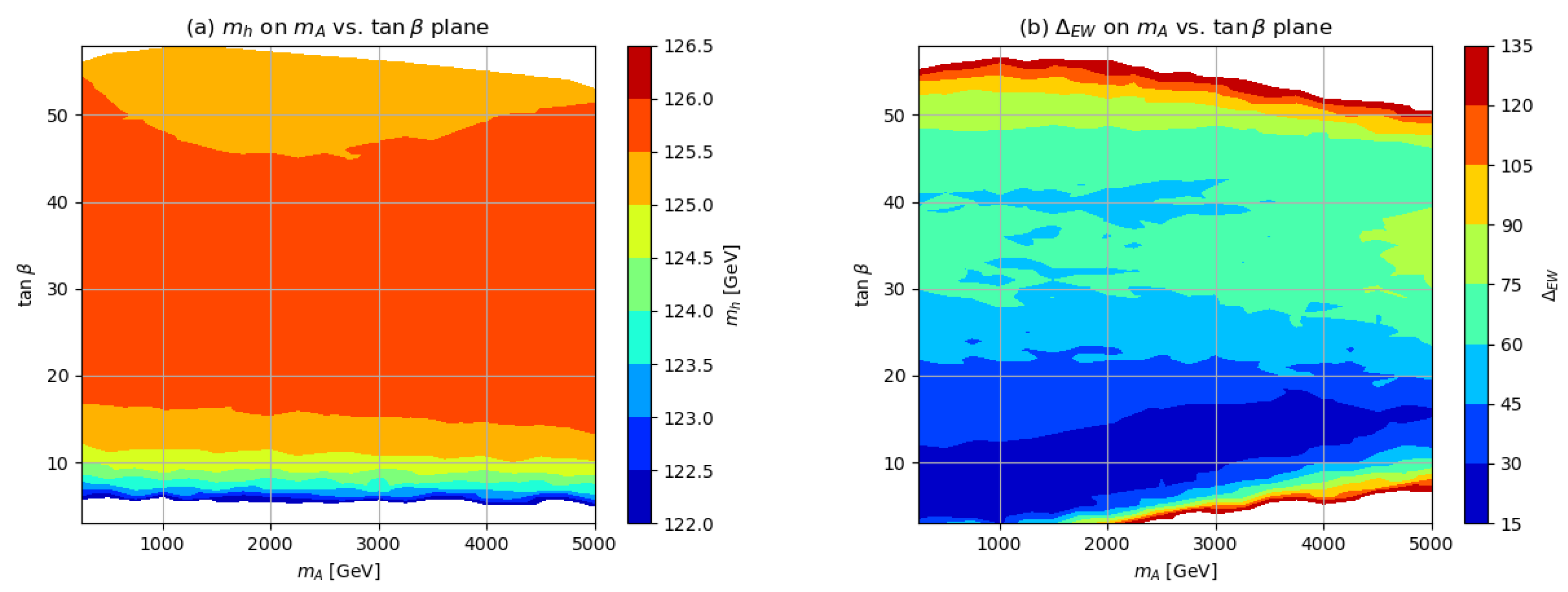
3. Production and Decay of $\mathit{H},\mathit{A}$ in the ${\mathit{m}}_{\mathit{h}}^{\mathbf{125}}\left(\mathrm{nat}\right)$ Scenario

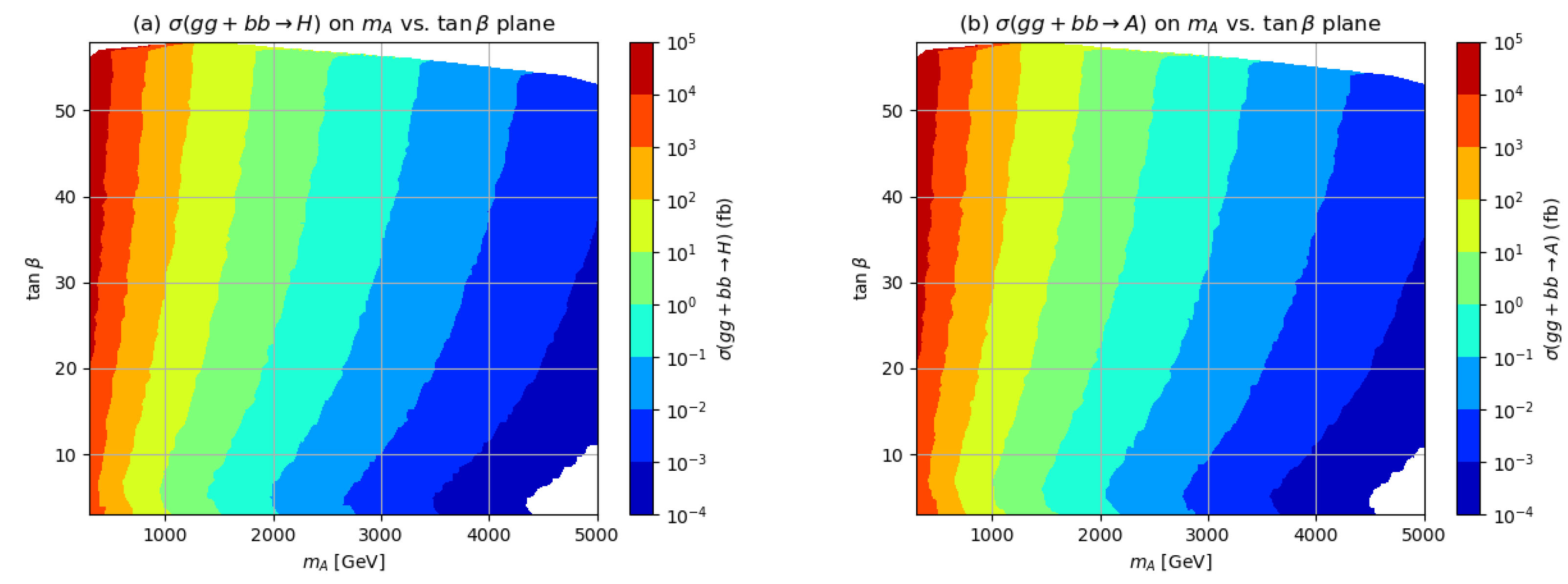
3.1. H and A Production Cross Sections in the $m_h^{125}\left(\mathrm{nat}\right)$ Scenario

The s-channel resonance production of the H and A bosons takes place mainly via $gg$ and $q\overline{q}$ (mainly $b\overline{b}$) fusion reactions at hadron colliders. The total H and A production cross sections are shown in the $m_A$ vs. $tan\beta$ plane in Figure 2 for $\sqrt{s}=14$ TeV $pp$ collisions—as are expected at CERN LHC Run 3 and at high-luminosity LHC (HL-LHC) where of order 300 fb⁻¹ (for Run 3) and 3000 fb⁻¹ (for HL-LHC) of integrated luminosity is expected to be obtained. For the cross sections, we use the computer code SusHi [49] which contains contributions up to NNLO in perturbative QCD. The cross sections range from over ${10}^4$ fb at low $m_{H,A}\sim 400$ GeV down to $\sigma (pp\to H,A)<1$ fb for $m_{H,A}\sim 2$ TeV, and they increase somewhat with increasing $tan\beta$ where production via $b\overline{b}$ fusion is enhanced.

Figure 2. The total cross section for (a) $pp\to H$ and (b) $pp\to A$ at $\sqrt{s}=14$ TeV using the SusHi code [49].

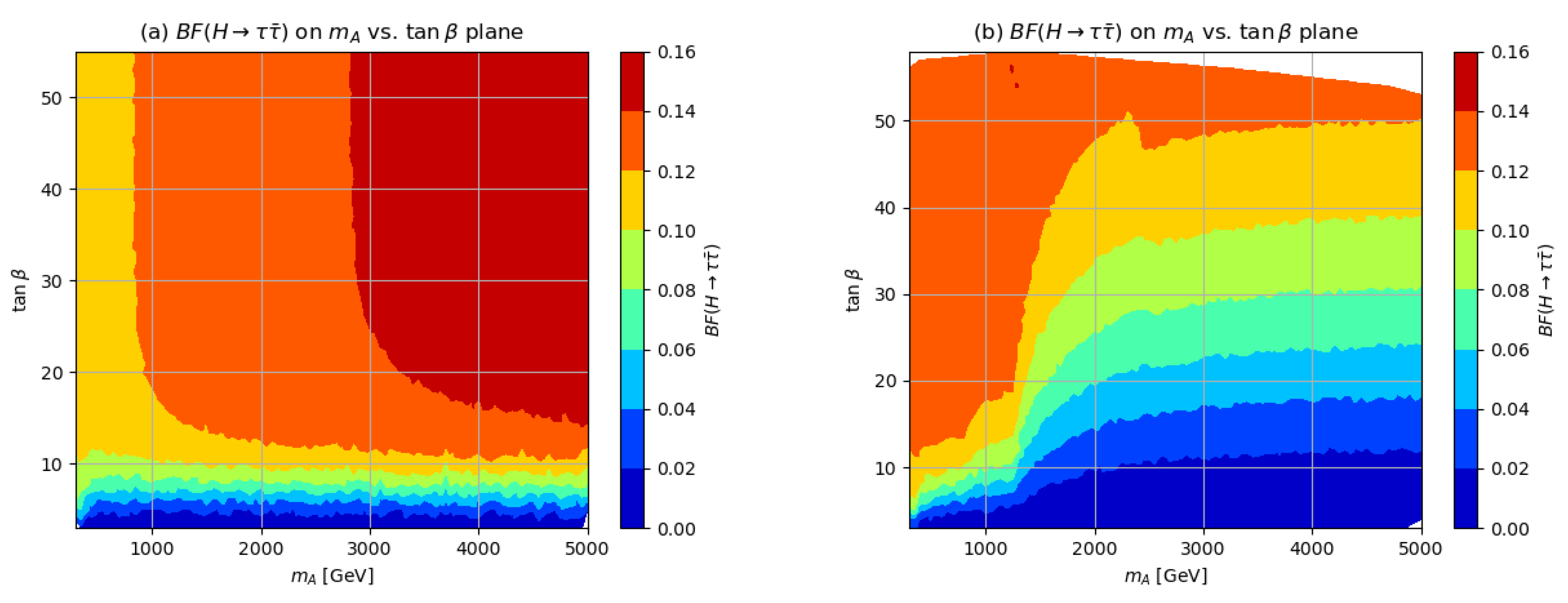
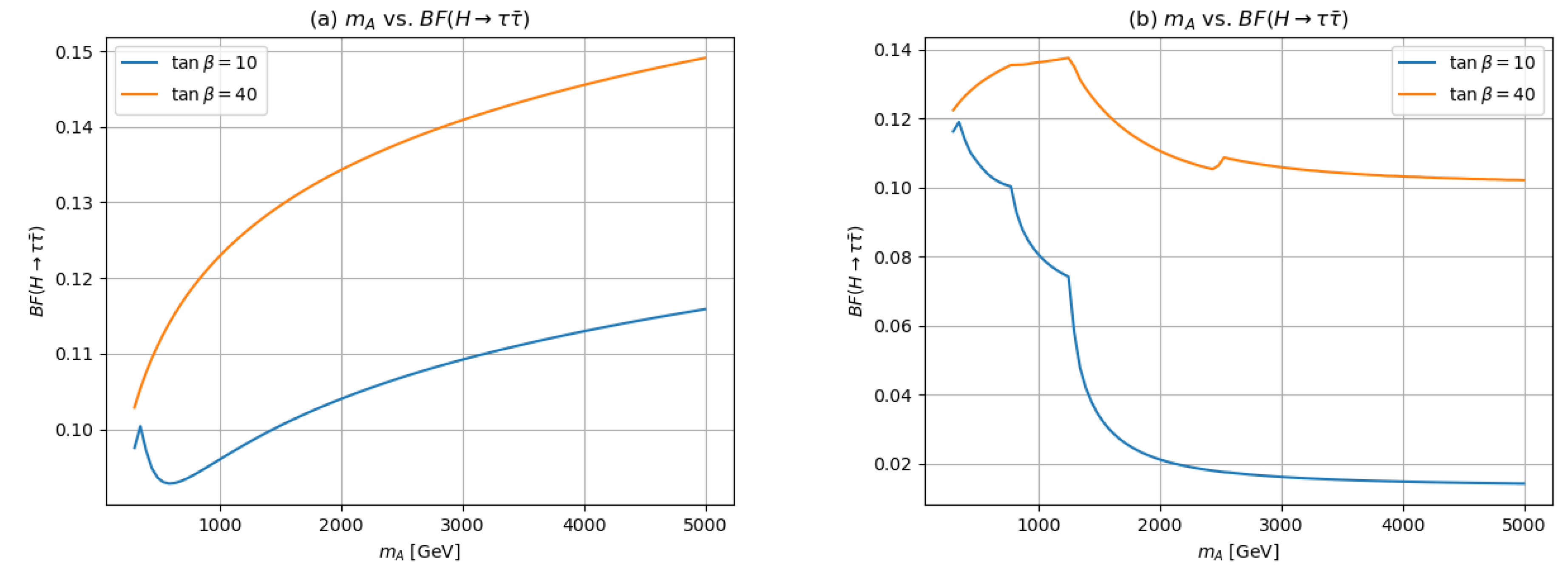
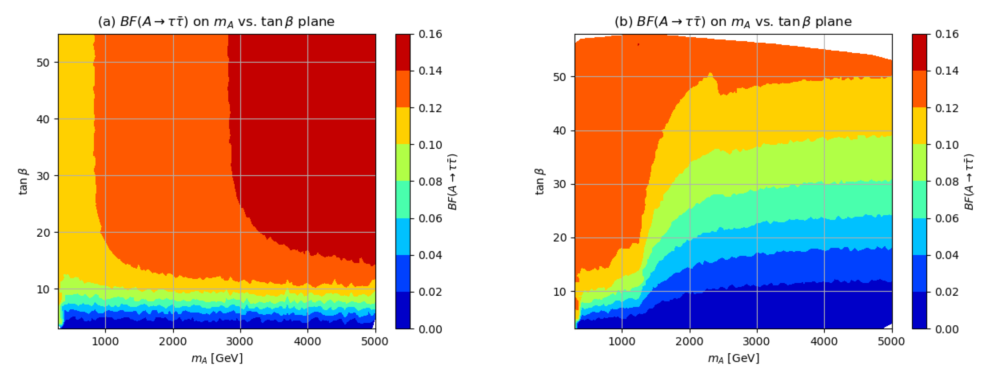
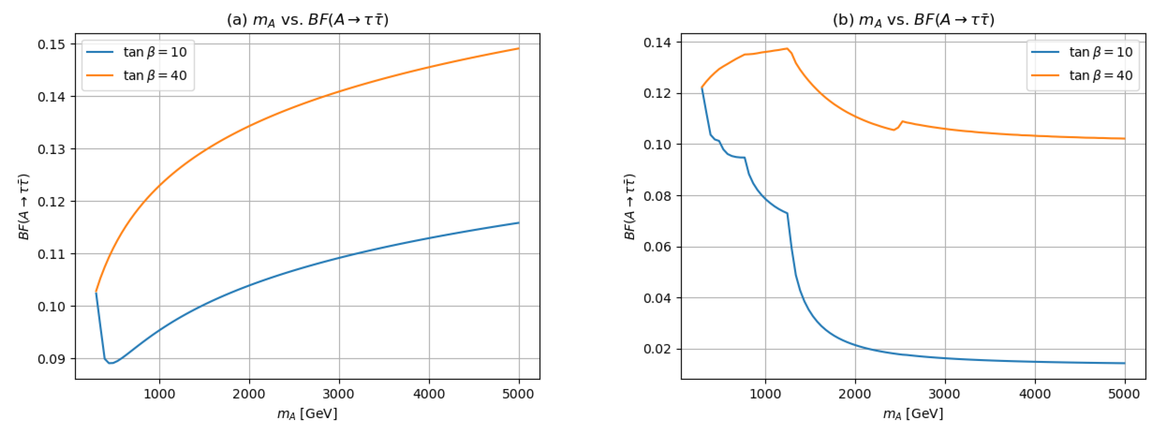
3.2. H and A Branching Fractions in the $m_h^{125}\left(\mathrm{nat}\right)$ Scenario

It is sometimes claimed in the literature that the tree-level production and decay rates for the H and A bosons depend only on $m_A$ and $tan\beta$, and indeed search limits for the heavy Higgs bosons are typically presented in the $m_A$ vs. $tan\beta$ plane, following the early pioneering work by Kunszt and Zwirner [50]. While this is true for the (non-supersymmetric) 2HDM, it is not true for the MSSM, where the importance of tree level SUSY Higgs boson decays to SUSY particles was first emphasized in [51,52,53]. In the 2HDM, decays of H and A to the heaviest available fermion pairs will typically dominate, with decays to $b\overline{b}$ and $\tau \overline{\tau }$ enhanced at large $tan\beta$. However, in SUSY models there is a direct gauge coupling

$$\mathcal{L}\ni -\sqrt{2}\sum _{i,A}{\mathcal{S}}_i^{†}g{t}_A{\overline{\lambda }}_A{\psi }_i+H.c.$$

(10)

where ${\mathcal{S}}_i$ labels various matter and Higgs scalar fields, ${\psi }_i$ is the fermionic superpartner of ${\mathcal{S}}_i$ and ${\lambda }_A$ is the gaugino with gauge index A. Furthermore, g is the corresponding gauge coupling for the gauge group in question and the $t_A$ are the corresponding gauge group matrices. Letting ${\mathcal{S}}_i$ be the Higgs scalar fields, we see there is an unsuppressed coupling of the Higgs scalars to gaugino plus higgsino. This coupling can lead to dominant SUSY Higgs boson decays to SUSY particles when the gaugino-plus-higgsino decay channel is kinematically unsuppressed.

In Figure 3, we plot the $H\to \tau \overline{\tau }$ branching fractions as color-coded regions in the $m_A$ vs. $tan\beta$ plane for (a) the hMSSM and (b) for our $m_h^{125}\left(\mathrm{nat}\right)$ BM scenario. For the hMSSM, we use the computer code 2HDMC [54] with $m_h=125$ GeV throughout the $m_A$ vs. $tan\beta$ plane but with decoupled sparticles. We use the “Physical mass input set”. With the potential parameters ${\lambda }_i$ as in the tree-level MSSM except ${\lambda }_2$, which includes a correction term to bring the light CP-even higgs mass to be 125 GeV, the only free physical inputs left are then just $m_A$ and $tan\beta$. From frame (a), we see as expected that for the hMSSM, the $BF(H\to \tau \overline{\tau })$ increases with $tan\beta$. It also increases slightly as $m_A$ increases since the $\tau$ Yukawa coupling $f_{\tau }$ increases slightly with scale choice. In frame (b) for the $m_h^{125}\left(\mathrm{nat}\right)$ case, we again see an increasing branching fraction as $tan\beta$ increases, but now as $m_A$ (and hence $m_H$) increases, various SUSY decay modes to EWinos open up, especially around $m_A\sim 1200$ GeV where decays to gaugino-plus-higgsino become accessible. We see the $BF(H\to \tau \overline{\tau })$ can drop from 12% on the left-side of the plot down to just a few percent on the right-hand-side. This is due to the fact that the decay to EWinos ultimately dominates the heavy Higgs branching fraction [55,56]. There is also a glitch apparent at around $m_A\sim 2500$ GeV in the contours. This occurs because we include SUSY threshold corrections to the Yukawa couplings which are implemented at the scale $m_{SUSY}^2=m_{{\tilde{t}}_1}{m}_{{\tilde{t}}_2}$ and so the Yukawa couplings have a slight discontinuity (see, e.g., Figure 6 of Ref. [57]).

Figure 3. Branching fraction of $H\to \tau \overline{\tau }$ in the (a) hMSSM and (b) in the $m_h^{125}\left(\mathrm{nat}\right)$ benchmark case in the $m_A$ vs. $tan\beta$ plane.

It is also helpful to show the explicit $BF(H\to \tau \overline{\tau })$ vs. $m_A$ for two specific choices of $tan\beta =10$ and 40 for the (a) hMSSM and (b) the $m_h^{125}\left(\mathrm{nat}\right)$ model in Figure 4. For the hMSSM, we again see the slight increase with increasing $m_A$, although the BFs stay in the vicinity of 10–15%. For the $m_h^{125}\left(\mathrm{nat}\right)$ case, we see the sharp drop off in $BF(H\to \tau \overline{\tau })$ as various $H\to EWinos$ thresholds are passed: then, ultimately the branching fraction drops below 2% for large $m_A$.

Figure 4. Branching fraction of $H\to \tau \overline{\tau }$ in the (a) hMSSM and (b) in the $m_h^{125}\left(\mathrm{nat}\right)$ benchmark case vs. $m_A$ for $tan\beta =10$ and 40.

Similar behavior is shown in Figure 5a,b for the $A\to \tau \overline{\tau }$ branching fraction: it has a slight increase with increasing $m_A$ for the hMSSM case but suffers sharp drops in the $m_h^{125}\left(\mathrm{nat}\right)$ case due to the turn on of A decay to gaugino-plus-higgsino. This will affect the reach plots in a substantial way.

Figure 5. Branching fraction of $A\to \tau \overline{\tau }$ in the (a) hMSSM and (b) in the $m_h^{125}\left(\mathrm{nat}\right)$ benchmark case in the $m_A$ vs. $tan\beta$ plane.

The corresponding plots of $BF(A\to \tau \overline{\tau })$ vs. $m_A$ for $tan\beta =10$ and 40 are shown in Figure 6. The behavior is rather similar to that already explained for the H decay.

Figure 6. Branching fraction of $A\to \tau \overline{\tau }$ in the (a) hMSSM and (b) in the $m_h^{125}\left(\mathrm{nat}\right)$ benchmark case vs. $m_A$ for $tan\beta =10$ and 40.

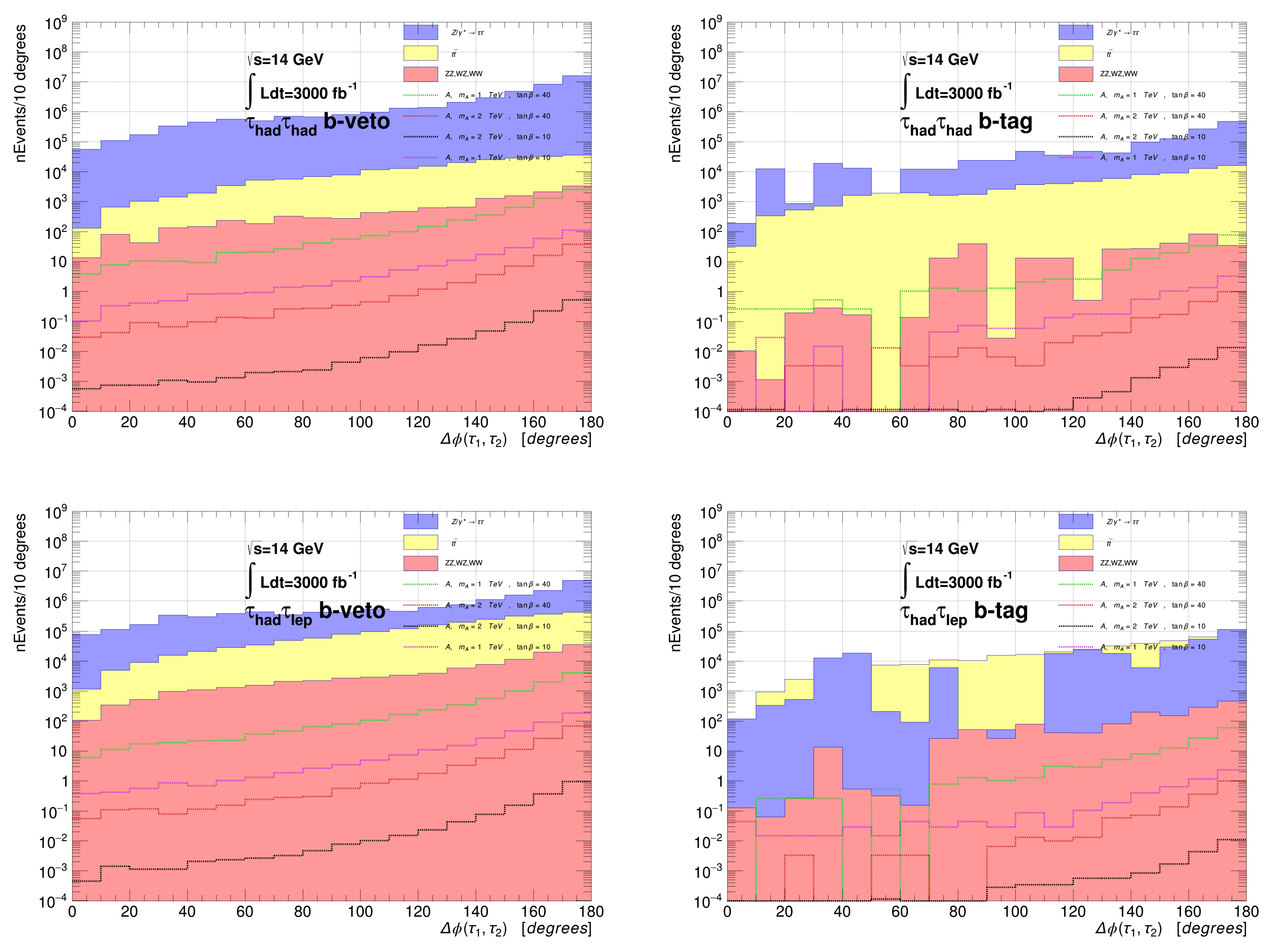
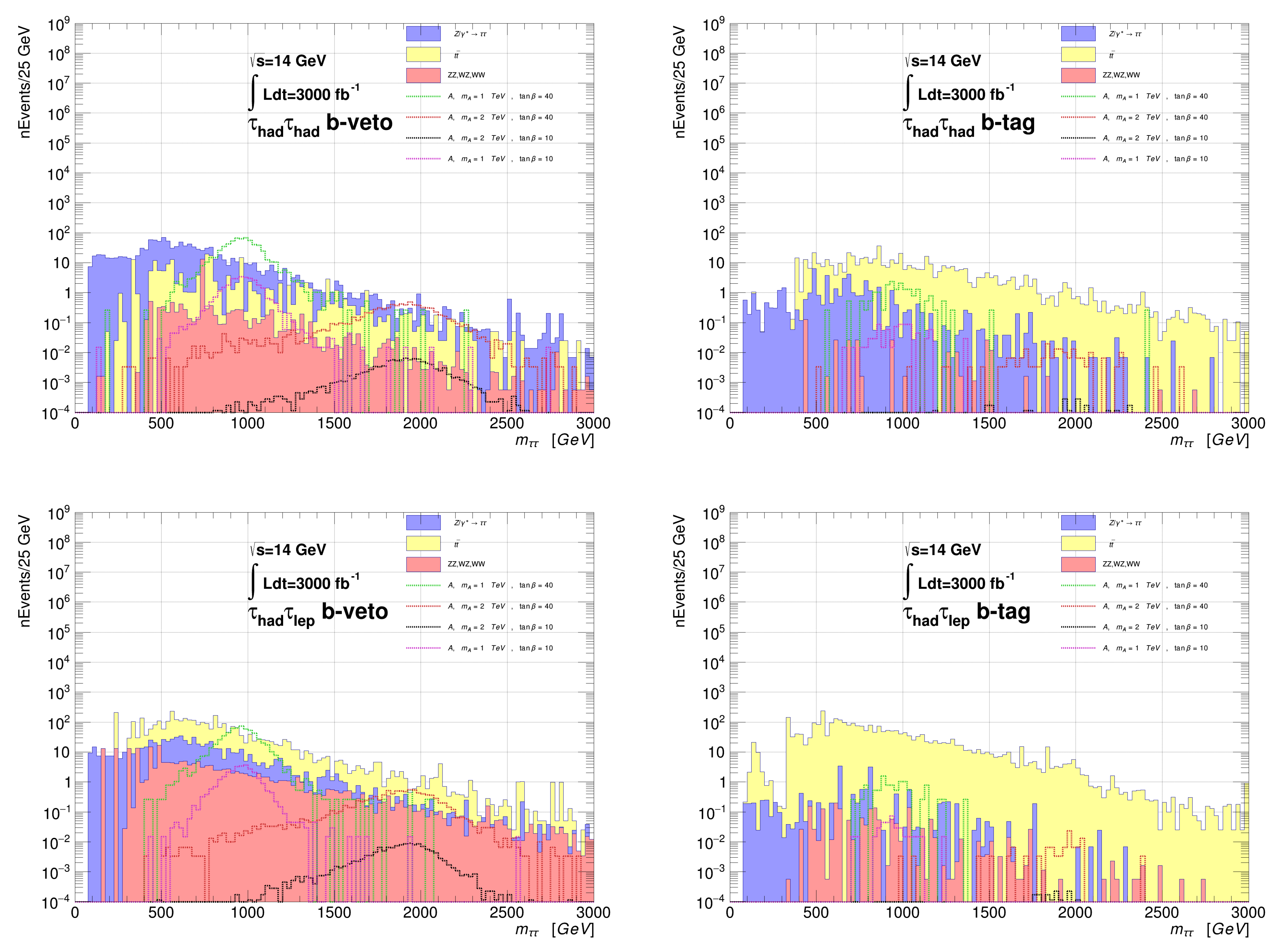
4. Signal from Back-to-Back $\mathbf{\tau }\overline{\mathbf{\tau }}$ via ${\mathbf{m}}_{\mathbf{T}}$

In this Section, we present details from our event generation calculations for the $H,A\to \tau \overline{\tau }$ signal with nearly back-to-back (BtB) $\tau$s. For signal and background event generation, we adopt the Pythia 8.07 event generator [58] interfaced with the Delphes toy detector simulation [59]. For signal, we generate $pp\to H,A\to \tau \overline{\tau }$ events with the total cross section adjusted to the SusHi NNLO result. For SM backgrounds, we generate $q\overline{q}\to {\gamma }^{*},Z\to \tau \overline{\tau }$ (Drell-Yan), $t\overline{t}$ and $VV$ production where $VV=W^{+}{W}^{-},W^{\pm }Z$ and $ZZ$.

For jet finding, we use the Delphes FASTJET jet finder. The FASTJET jet finder requires $p_T\left(jet\right)>25$ GeV and $\Delta R$ between jets as $\Delta R_{jj}>0.4$. We also require $|{\eta }_{jet}|<2.5$. Delphes includes a hadronic $\tau$-jet finding tool which we also use which identifies one-and-three charged prong jets as tau jets provided the tau is within $\Delta R=0.4$ of the jet in question. The Delphes $\tau$-jet identification efficiency is found to be in the 50% range which is well below the ATLAS quoted $\tau$-jet efficiency ID which is at the 75% level. We also use the Delphes b-tag algorithm and the Delphes isolated lepton tag which requires $\Delta R(l,l)>0.3$ with $\left|\eta \right(e,\mu \left)\right|<2.5$.

The ${\tau }_{had}{\tau }_{had}$ channel are selected by single-$\tau$ trigger $p_T$ cut of 160 GeV. Events contain at least two ${\tau }_{had}$ identified by the Delphes tau-tag algorithm. The two tau ${\tau }_{had}$ candidates must have opposite electric charge.

The ${\tau }_{lep}{\tau }_{had}$ channel are selected using single-electron and single-muon triggers with $p_T$ threshold of 30 GeV. The events contain exactly one isolated lepton and at least one ${\tau }_{had}$ candidate. The isolated lepton and the ${\tau }_{had}$ candidate must have opposite electric charge. Furthermore, we rejected the events that the isolated lepton and the ${\tau }_{had}$ candidate have an invariant mass between 80 GeV and 110 GeV to reduce the background contribution from $Z\to ee$.

The events from either channel are further divided into categories of the b-tag for events containing at least one b-jet and the b-veto for events containing no b-jets.

After selecting for candidate ditau events, we plot in Figure 7 the transverse opening angle $\Delta \varphi \left(\tau \overline{\tau }\right)$ from our signal and BG events for our $m_h^{125}\left(\mathrm{nat}\right)$ benchmark point with $m_A=1$ and 2 TeV and $tan\beta =10$ and 40. Both the DY background and the signal events rise to a peak at ${180}^{\circ }$ indicating that these events are mostly back-to-back in the transverse plane as expected. The ditau opening angle from $t\overline{t}$ and $VV$ are rather less pronounced at $\Delta \varphi \sim {180}^{\circ }$.

Figure 7. Distribution in transverse ditau opening angle $\Delta \varphi \left(\tau \tau \right)$ for our $m_h^{125}\left(\mathrm{nat}\right)$ benchmark scenario with $tan\beta =10$ and $m_A=1$ and 2 TeV.

We next divide our signal into BtB ditau events, where $\Delta \varphi \left(\tau \overline{\tau }\right)>{155}^{\circ }$ (this Section) or non-BtB (acollinear) ditaus where $\Delta \varphi \left(\tau \tau \right)<{155}^{\circ }$ (Section 5).

Then we plot the total transverse mass variable $m_T^{tot}$ as shown in Figure 8. From the plot, we see that the signal distributions rise to a peak around $m_T\sim 0.8m_A$ and then fall off sharply for $m_T\gtrsim m_A$ due to kinematics (the cutoff is not completely sharp due to considerable smearing entering into the signal distributions). The SM backgrounds are all peaked below $m_T\sim 500$ GeV and have falling distributions for increasing values of $m_T^{tot}$.

Figure 8. Distribution in $m_T^{tot}$ for ditau events with $\Delta \varphi \left(\tau \tau \right)>{155}^{\circ }$ for our $m_h^{125}\left(\mathrm{nat}\right)$ benchmark scenario with $tan\beta =10$ and $m_A=1$ and 2 TeV after cuts listed in the text.

5. Signal from Acollinear $\mathbf{\tau }\overline{\mathbf{\tau }}$ via ${\mathbf{m}}_{\mathbf{\tau }\mathbf{\tau }}$

For acollinear ditau events (non-BtB), we require the transverse ditau opening angle $\Delta \varphi \left(\tau \tau \right)<{155}^{\circ }$ so that this data set is orthogonal to the back-to-back ditau set. For the acollinear ditau events, we also require the presence of an additional jet in the event besides the ${\tau }_{had}$ jets (usually an initial-state-radiation (ISR) jet in the case of signal events): $n_{jets}\ge 1$. For this configuration, then we are able to use the tau-tau invariant mass reconstruction trick since once ${\overrightarrow{E}}_T^{miss}$ is known, and we assume the neutrinos from each tau decay are collinear with the parent tau direction, then the ditau invariant mass can be solved for. Since the taus are ultra-relativistic, the daughter visible decay products and the associated neutrinos are all boosted in the direction of the parent $\tau$ momentum. In the approximation that the visibles (vis) and the neutrinos from the decay of each tau are all exactly collimated in the tau direction, we can write the momentum carried off by the neutrinos from the decay ${\tau }_1\to vi{s}_1\nu$ of the first tau as ${\xi }_1{\overrightarrow{p}}_T\left(vi{s}_1\right)$ and likewise for the second tau. Momentum conservation in the transverse plane requires

$$-{\overrightarrow{p}}_T\left(j\right)=(1+{\xi }_1){\overrightarrow{p}}_T\left(vi{s}_1\right)+(1+{\xi }_2){\overrightarrow{p}}_T\left(vi{s}_2\right).$$

(11)

Since this is really two independent equations (recall we require $p_T\left(j\right)>25$ GeV), it is possible to use the measured values of the jet and visible-tau-decay momenta to solve these to obtain ${\xi }_1$ and ${\xi }_2$, event-by-event. It is simple to check that in the approximation of collinear tau decay, the squared mass of the di-tau system is given by

$$m_{\tau \tau }^2=(1+{\xi }_1)(1+{\xi }_2)m_{vi{s}_{1}vi{s}_2}^2$$

(12)

For ditau plus jet events from $H,A$-decay to taus, we expect ${\xi }_i>0$ and $m_{\tau \tau }^2$ to peak at $m_{H,A}^2$. Moreover, for these events, the missing energy vector will usually point in between the two $\tau \left(vis\right)$ momentum vectors in the transverse plane. In contrast, for backgrounds where $E_T^{miss}$ arises from neutrinos from decays of heavy SM particles (t, W, Z), the visible and $E_T^{miss}$ directions are uncorrelated and the $E_T^{miss}$-vector may point well away, or even backwards, from one of the leptons so that one (or both) ${\xi }_i<0$.

Then we can plot the $m_{\tau \tau }$ distribution, as is shown in Figure 9 for $tan\beta =10$ and 40 and for (a) $m_A=1$ TeV and (b) $m_A=2$ TeV. From the plot, the DY distribution shows a remnant peak at $m_Z=91.2$ GeV while $t\overline{t}$ and $VV$ are peaked below 500 GeV. In contrast, the $A\to \tau \overline{\tau }$ signal distributions are peaked at $m_{\tau \tau }\sim m_A$ with a width that arises from smearing effects and non-exact-collinearity of the $\tau$ decay products.

Figure 9. Distribution in $m_{\tau \tau }$ for ditau events with $\Delta \varphi \left(\tau \tau \right)<{155}^{\circ }$ and $n_{jet}\ge 1$ for our $m_h^{125}\left(\mathrm{nat}\right)$ benchmark scenario with $tan\beta =10$ and a) $m_A=1$ and b) $m_A=2$ TeV after cuts listed in the text.

To illustrate some numerics of our results, in Table 2 we list the resultant signal and background cross sections (in fb) after all cuts for the cases of $pp\to H,A\to \tau \overline{\tau }$ at $\sqrt{s}=14$ TeV for $tan\beta =10$ and $m_A=1$ TeV, for both the hMSSM and the $m_h^{125}\left(\mathrm{nat}\right)$ scenario. From the Table, we see that, as expected, the surviving signal after cuts from the $m_h^{125}\left(\mathrm{nat}\right)$ scenario is somewhat diminished from the hMSSM case due to the diminished branching fractions $BF(H,A\to \tau \overline{\tau })$. Furthermore, the two signal channels from H and from A production are nearly comparable. The dominant background comes from ${\gamma }^{*},Z\to \tau \overline{\tau }$ while $t\overline{t}$ and $VV$ are smaller but still significant. The signal is quite smaller in the acollinear channel than in the BtB channel. However, this is compensated for somewhat by smaller backgrounds in the acollinear channel than in the BtB channel, which makes the acollinear channel to have a much better $S/B$ ratio than the BtB channel.

Table 2. Cross section (fb) after optimized cuts for the various signal and background processes from $pp$ collisions at $\sqrt{s}=14$ TeV and $tan\beta =10$ and $m_A=1$ TeV.

Process	Back-to-Back (BtB)	Acollinear
$H\to \tau \overline{\tau }\left(\mathrm{hMMSSM}\right)$	0.197	0.024
$A\to \tau \overline{\tau }\left(\mathrm{hMMSSM}\right)$	0.222	0.027
$H\to \tau \overline{\tau }\left(\mathrm{SUSY}\right)$	0.140	0.017
$A\to \tau \overline{\tau }\left(\mathrm{SUSY}\right)$	0.162	0.020
${\gamma }^{*},Z\to \tau \overline{\tau }$	23.33	0.586
$t\overline{t}$	19.95	2.112
$VV$	0.663	0.069
$total\left(BG\right)$	43.94	2.767

6. Reach of LHC3 and HL-LHC for $\mathit{H},\mathit{A}\to \mathit{\tau }\overline{\mathit{\tau }}$

After settling on cuts for the BtB and acollinear ditau signals, it is possible to plot reach plots in terms of exclusion limits or discovery sensitivity for $pp\to H,A\to \tau \overline{\tau }$ in the $m_A$ vs. $tan\beta$ plane.

For the exclusion plane, the upper limits for exclusion of a signal are set at the 95% CL and assume the true distribution one observes in experiment corresponds to background only. They are then computed using a modified frequentist $C{L}_s$ method [60] with the profile likelihood ratio as the test statistic.

For the discovery plane, we use $5\sigma$ to denote the discovery and assume the true distribution one observes in experiment corresponds to signal-plus-background. Then we test this against the background only distribution to see if the background only hypothesis could be rejected at a $5\sigma$ level. Specifically, we use the binned $m_T^{tot}$ distribution (Figure 8) for the BtB events and the $m_{\tau \tau }$ distribution (Figure 9) for acollinear events to obtain the exclusion/discovery limits.

In both the exclusion plane and the discovery plane, the asymptotic approximation for getting the median significance is used [61]. The systematic uncertainty is assumed to be $1\sigma$ of the corresponding statistical uncertainty, which is a very conservative rule-of-thumb estimate.

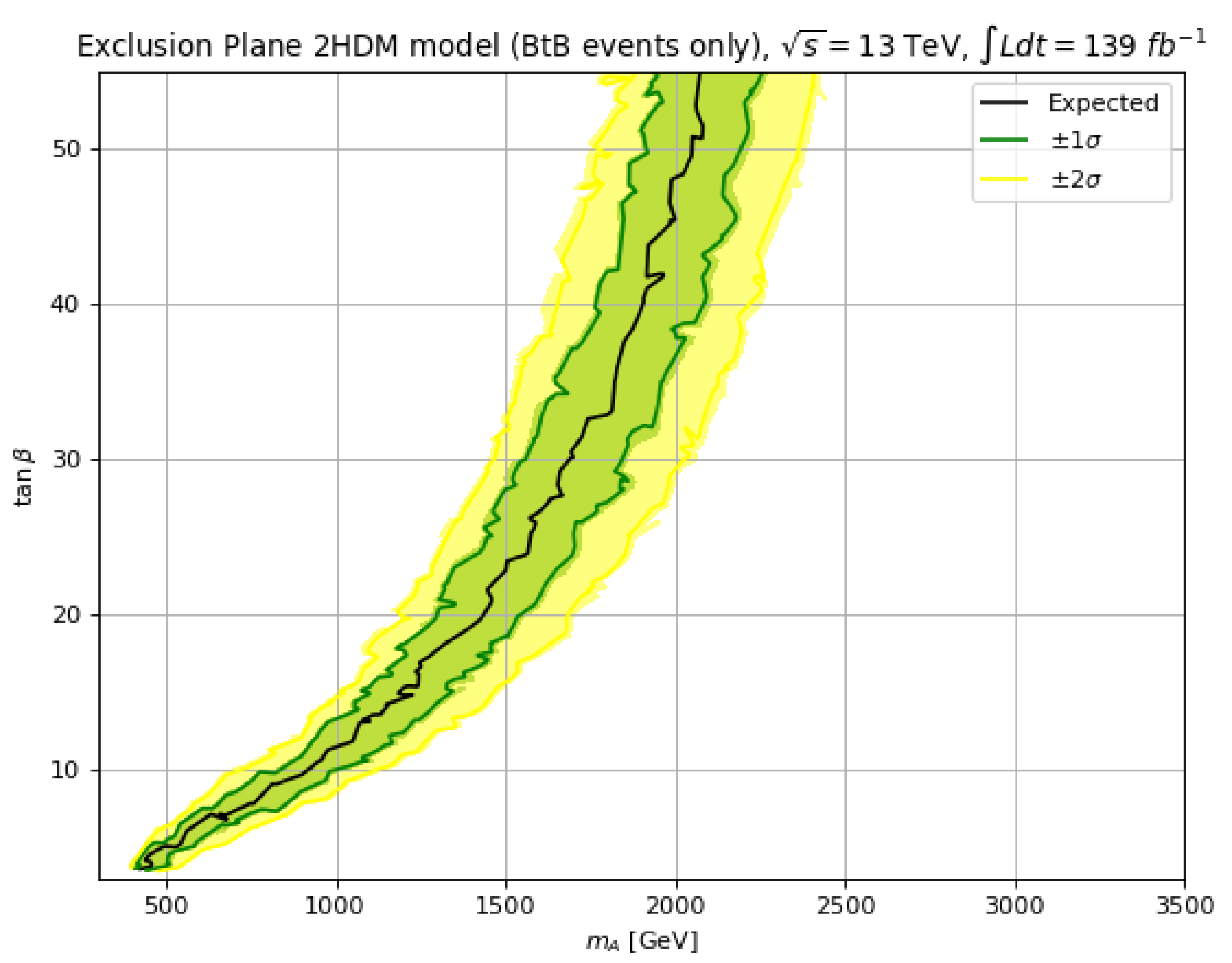
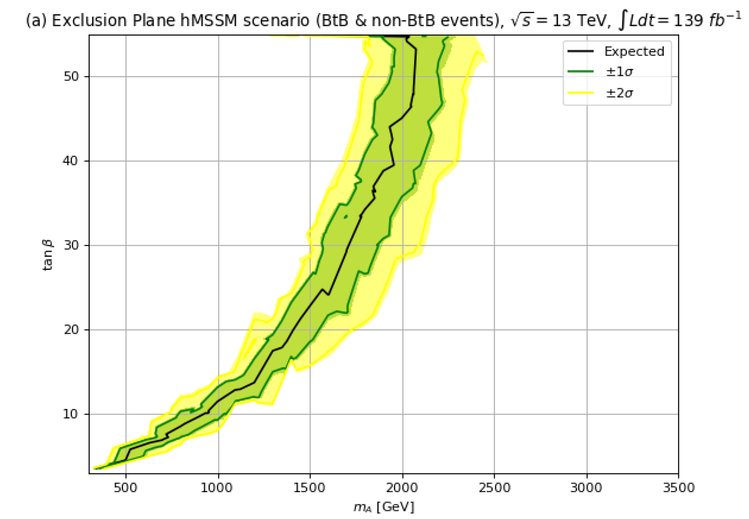
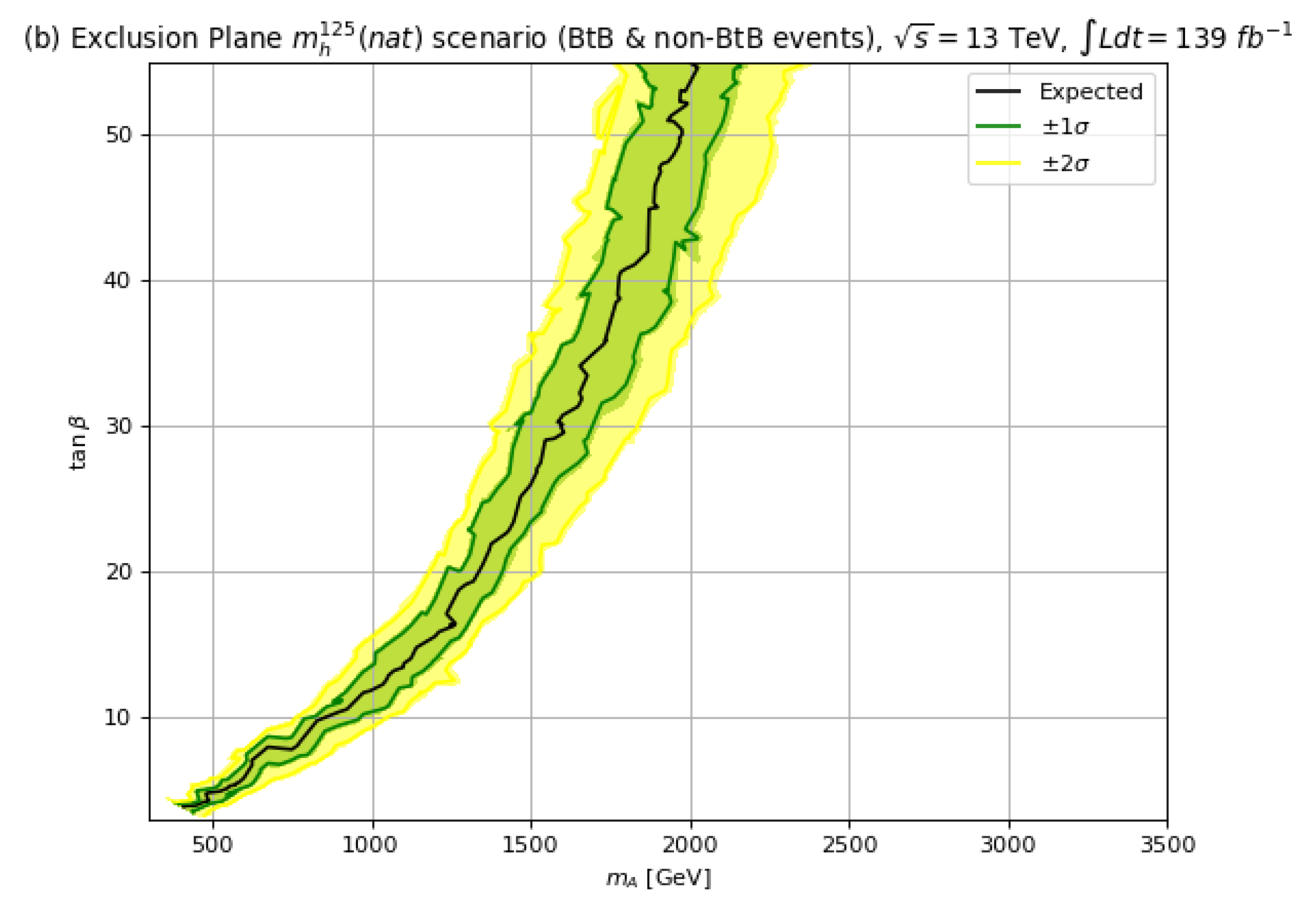
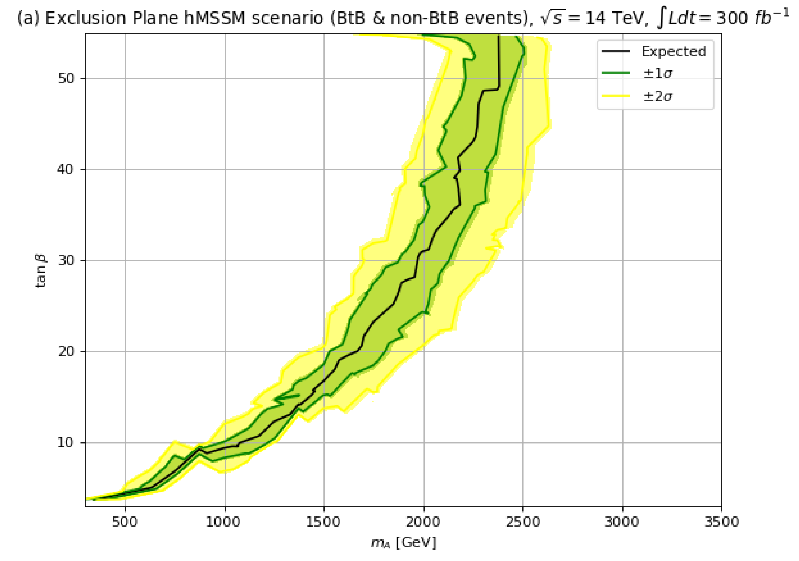
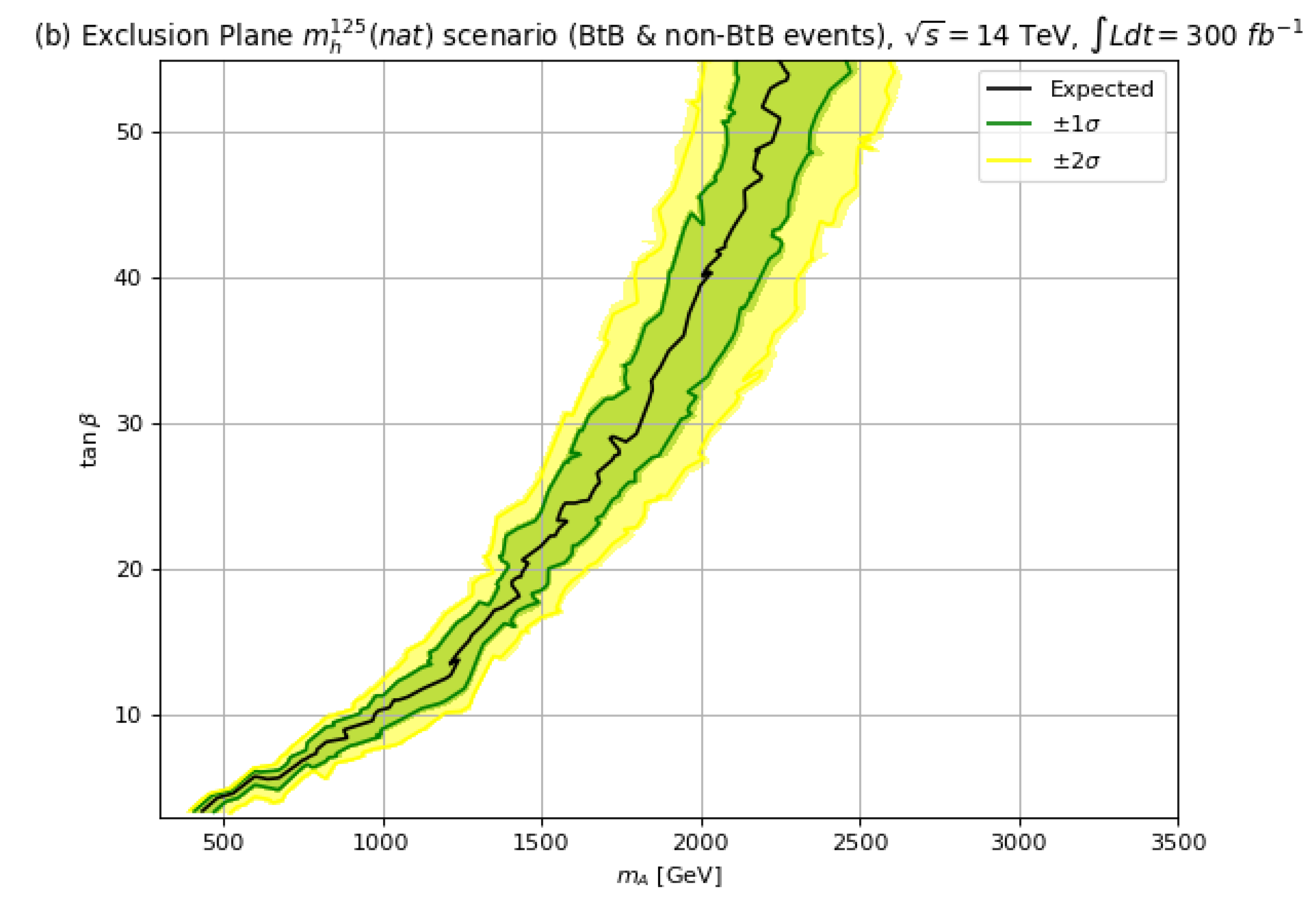
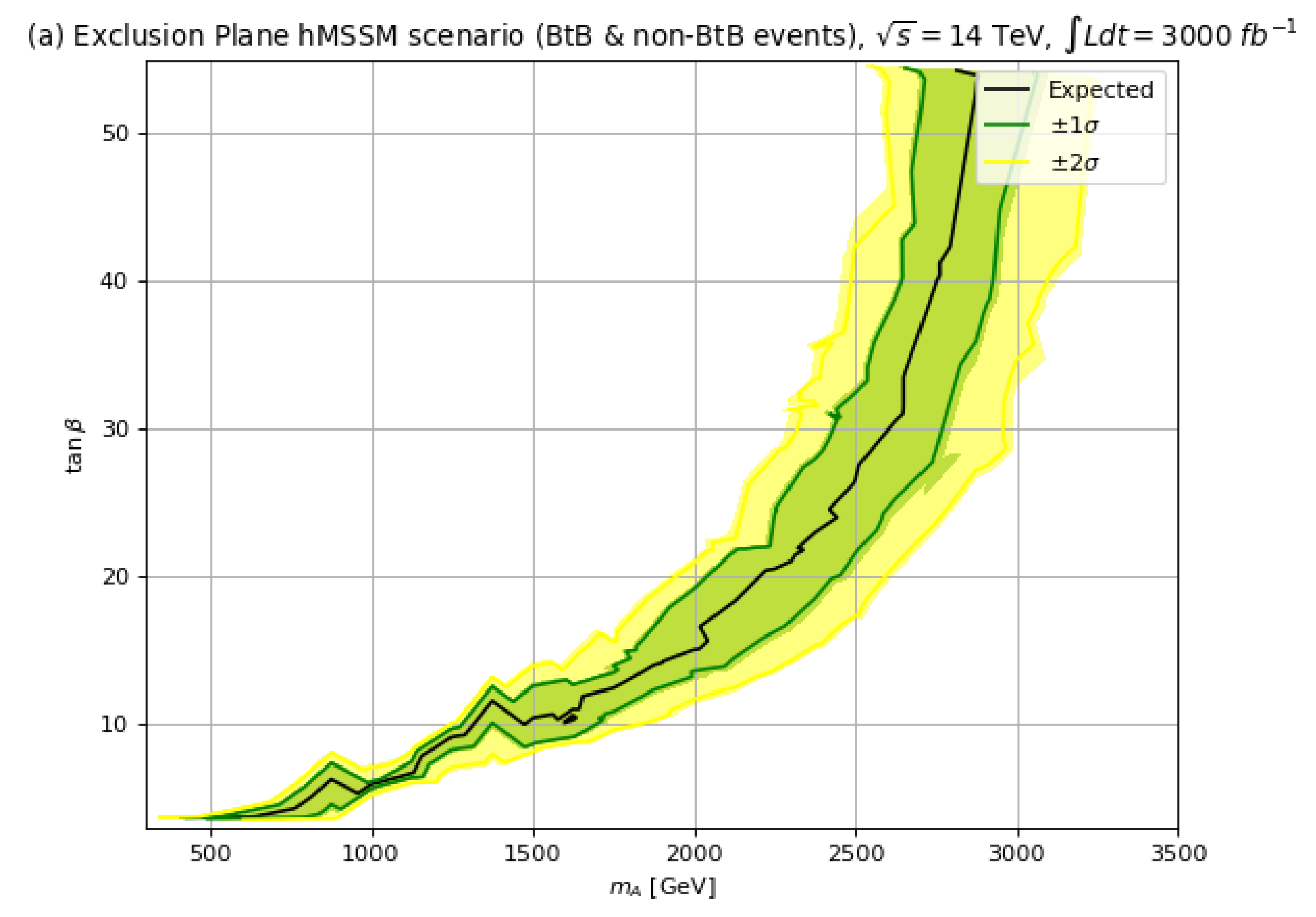
6.1. Exclusion Plane

As a first step, to compare with the ATLAS reach of upper limits obtained in their Run 2 search with 139 fb⁻¹, we plot our corresponding exclusion limit in Figure 10. For this plot, we use only the BtB signal in the hMSSM where $m_h$ is set to 125 GeV, which should compare well with the $m_h^{125}$ scenario used by ATLAS which contains sparticles at or around 2 TeV, i.e., presumably SUSY decay modes are closed for most $m_A$ values shown in the plot. From Figure 10, we see our expected 95% CL exclusion extends to $m_A\sim 0.9$ TeV for $tan\beta =10$ which compares favorably with ATLAS. For $tan\beta =40$, we obtain a 95% CL exclusion of $m_A\sim 1.9$ TeV, which is somewhat better than the ATLAS expected result of $m_A\sim 1.8$ TeV.

Figure 10. The 95% CL upper limits with $\sqrt{s}=13$ TeV and 139 fb⁻¹ for $H,A\to \tau \overline{\tau }$ using BtB signal only in the hMSSM.

In Figure 11, we plot in frame (a) our expected Run 2 exclusion assuming 139 fb⁻¹ using the combined BtB and acollinear signal channels in the hMSSM. The exclusion limit extends to $m_A\sim 0.95$ TeV for $tan\beta =10$ and to $m_A\sim 1.95$ TeV for $tan\beta =40$. For frame (b), for the $m_h^{125}\left(\mathrm{nat}\right)$ scenario, then the corresponding 139 fb⁻¹ reach extends to $m_A\sim 0.8$ TeV for $tan\beta =10$ and to $m_A\sim 1.8$ TeV for $tan\beta =40$.

Figure 11. The 95% CL upper limits with $\sqrt{s}=13$ TeV and 139 fb⁻¹ for $H,A\to \tau \overline{\tau }$ in the (a) the hMSSM and (b) the $m_h^{125}\left(\mathrm{nat}\right)$ scenario.

In Figure 12, we present our projected future exclusion plots, this time for LHC collisions at $\sqrt{s}=14$ TeV with 300 fb⁻¹ of integrated luminosity, as would be expected from LHC Run 3. Here, we use both the BtB and acollinear signals. For Run 3, we see in frame (a) for the hMSSM with $tan\beta =10$, the 95% CL exclusion extends out to $m_A\sim 1.1$ TeV while the $tan\beta =40$ exclusion extends to $m_A\sim 2.3$ TeV. For the frame (b) case with the $m_h^{125}\left(\mathrm{nat}\right)$ scenario, the 95% CL reach for $tan\beta =10$ extends to $m_A\sim 1$ TeV whilst for $tan\beta =40$ the Run 3 exclusion extends to $m_A\sim 2$ TeV. Thus, comparing the Run 2 139 fb⁻¹ exclusion to that expected from LHC Run 3, we find an extra gain in exclusion of $m_A$ of ∼0.1–0.2 TeV. The presence of (natural) SUSY decay modes tends to reduce the LHC exclusion by ∼0.2 TeV compared to the hMSSM.

Figure 12. The 95% CL upper limits with $\sqrt{s}=14$ TeV and 300 fb⁻¹ for $H,A\to \tau \overline{\tau }$ in (a) the hMSSM and (b) the $m_h^{125}\left(\mathrm{nat}\right)$ scenario.

In Figure 13, we plot our projected exclusion limits of HL-LHC for $H,A\to \tau \overline{\tau }$ at $\sqrt{s}=14$ TeV with 3000 fb⁻¹. From frame (a) in the hMSSM case, we find a HL-LHC 95% CL exclusion out to $m_A\sim 1.5$ TeV for $tan\beta =10$ and out to $m_A\sim 2.8$ TeV for $tan\beta =40$. If instead we invoke the $m_h^{125}\left(\mathrm{nat}\right)$ SUSY scenario, then the corresponding HL-LHC exclusion drops to $m_A\sim 1.3$ TeV for $tan\beta =10$ and to $m_A\sim 2.6$ TeV for $tan\beta =40$, i.e., a drop in reach of about $0.2$ TeV in moving from the hMSSM to the $m_h^{125}\left(\mathrm{nat}\right)$ scenario.

Figure 13. The 95% CL upper limits with $\sqrt{s}=14$ TeV and 3000 fb⁻¹ for $H,A\to \tau \overline{\tau }$ in (a) the hMSSM and (b) the $m_h^{125}\left(\mathrm{nat}\right)$ scenario.

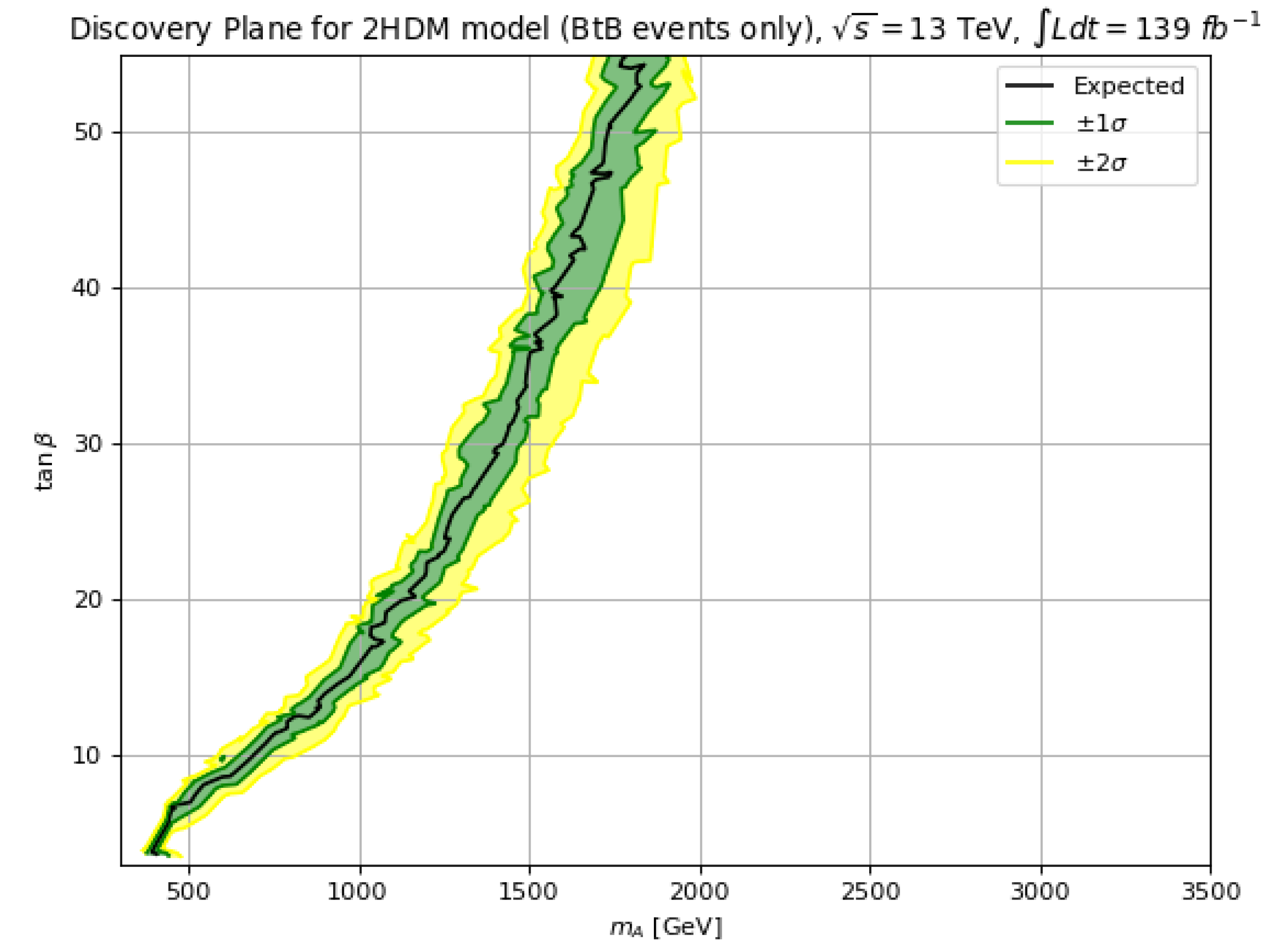
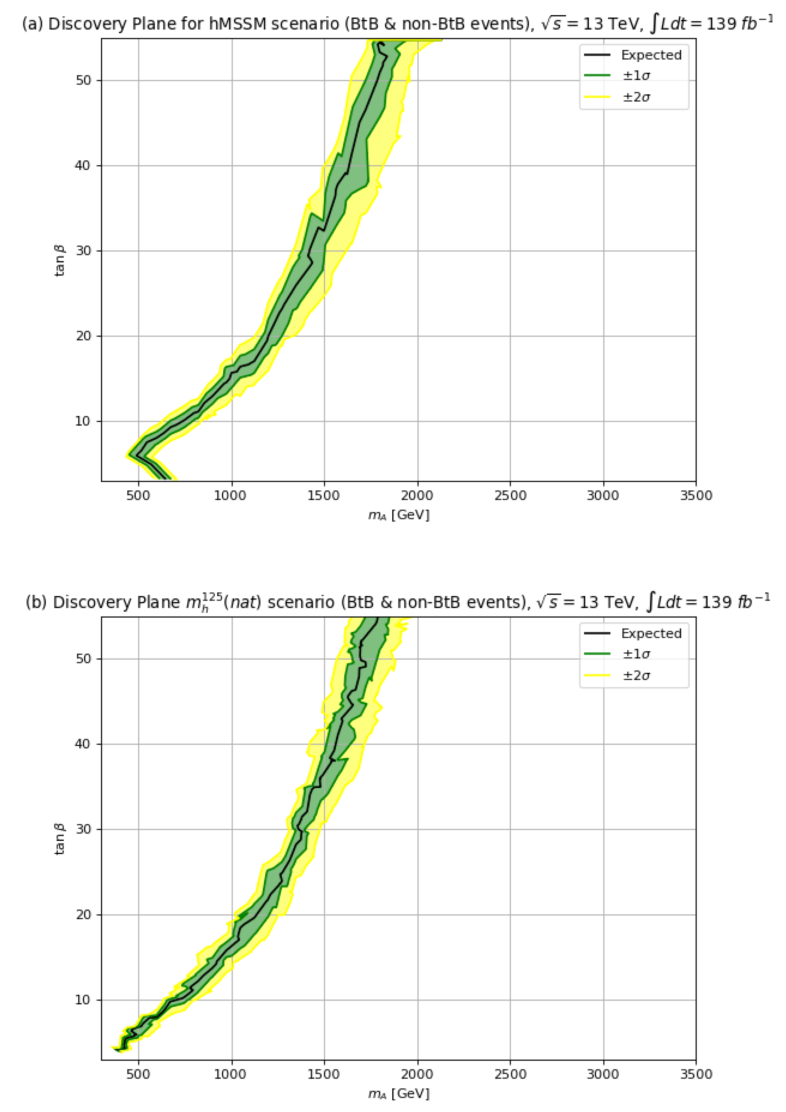
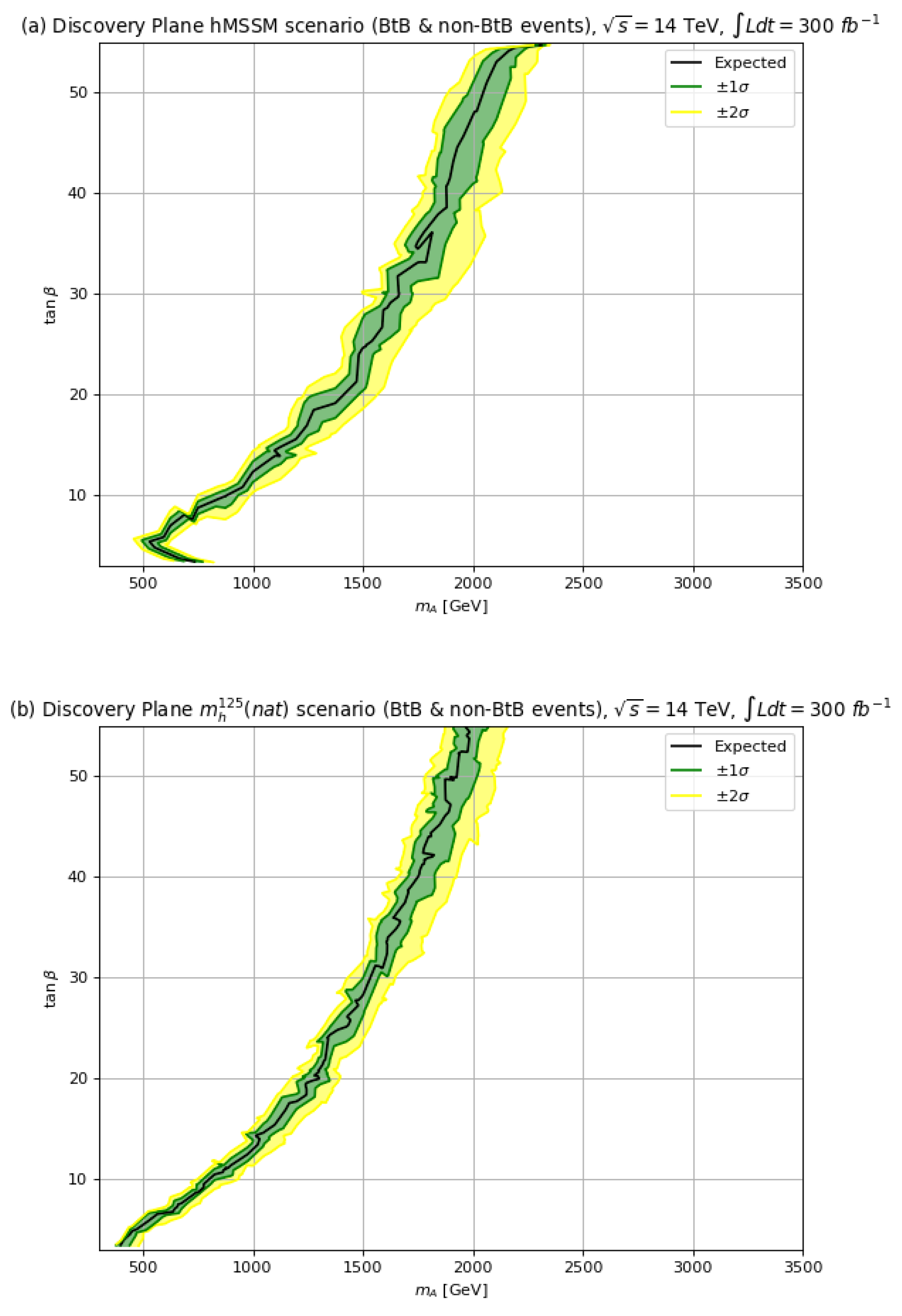
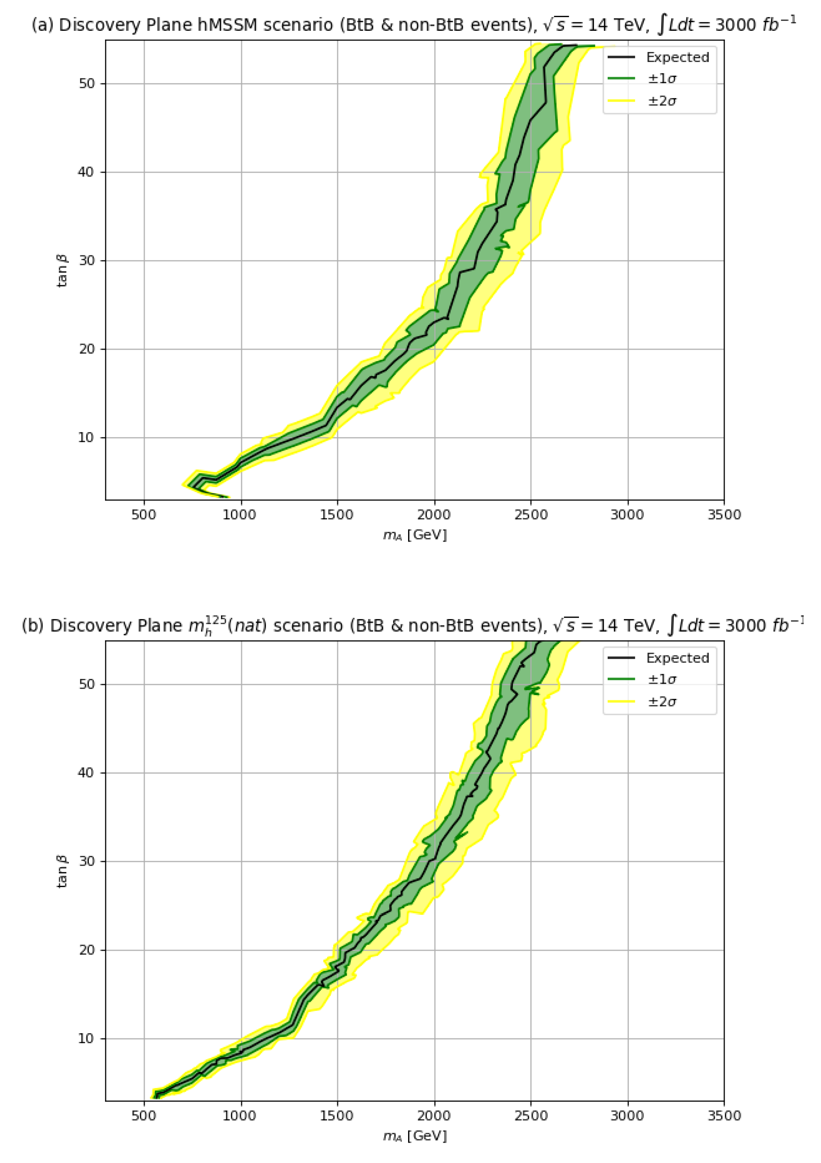
6.2. Discovery Plane

To compare with the ATLAS reach in the discovery plane obtained in their Run 2 search with 139 fb⁻¹, we show our corresponding results in Figure 14. For this plot, we use only the BtB signal in the hMSSM where $m_h$ is set to 125 GeV, which should compare well with the $m_h^{125}$ scenario used by ATLAS which contains sparticles at or around 2 TeV, i.e., presumably SUSY decay modes are closed for most $m_A$ values shown in the plot. From Figure 14, we see our expected $5\sigma$ reach extends to $m_A\sim 0.75$ TeV for $tan\beta =10$ which compares favorably wih ATLAS. For $tan\beta =40$, we obtain a $5\sigma$ reach of $m_A\sim 1.7$ TeV, which is somewhat better than the ATLAS expected reach of $m_A\sim 1.6$ TeV.

Figure 14. The discovery sensitivity at $5\sigma$ level with $\sqrt{s}=13$ TeV and 139 fb⁻¹ for $H,A\to \tau \overline{\tau }$ using BtB signal only in the hMSSM.

In Figure 15, we plot in frame (a) our expected Run 2 discovery reach assuming 139 fb⁻¹ using the combined BtB and acollinear signal channels in the hMSSM. The $5\sigma$ discovery reach for $tan\beta =10$ extends to $m_A=0.7$ TeV and for $tan\beta =40$ to $m_A=1.7$ TeV. For frame (b), for the $m_h^{125}\left(\mathrm{nat}\right)$ scenario, then the corresponding 139 fb⁻¹$5\sigma$ discovery reach extends to $m_A\sim 0.7$ TeV for $tan\beta =10$ and to $m_A\sim 1.6$ TeV for $tan\beta =40$.

Figure 15. The discovery sensitivity with $\sqrt{s}=13$ TeV and 139 fb⁻¹ for $H,A\to \tau \overline{\tau }$ in the (a) the hMSSM and (b) the $m_h^{125}\left(\mathrm{nat}\right)$ scenario.

In Figure 16, we present our future $5\sigma$ discovery sensitivity reach, this time for LHC collisions at $\sqrt{s}=14$ TeV with 300 fb⁻¹ of integrated luminosity, as would be expected from LHC Run 3. Here, we use both the BtB and acollinear signals. For Run 3, we see in frame (a) for the hMSSM the $tan\beta =10$ discovery reach extends out to $m_A\sim 0.8$ TeV while the $tan\beta =40$ reach extends to $m_A\sim 1.8$ TeV. For the frame b) case with the $m_h^{125}\left(\mathrm{nat}\right)$ scenario, the discovery sensitivity reach for $tan\beta =10$ extends to $m_A\sim 0.75$ TeV whilst for $tan\beta =40$ the Run 3 reach extends to $m_A\sim 1.75$ TeV. Thus, comparing the Run 2 139 fb⁻¹ reach to that expected from LHC Run 3, we find an extra gain in reach of $m_A$ of ∼0.1–0.2 TeV. The presence of (natural) SUSY decay modes tends to reduce the LHC reach by $\sim 0.1$ TeV compared to the hMSSM.

Figure 16. The discovery sensitivity with $\sqrt{s}=14$ TeV and 300 fb⁻¹ for $H,A\to \tau \overline{\tau }$ in (a) the hMSSM and (b) the $m_h^{125}\left(\mathrm{nat}\right)$ scenario.

In Figure 17, we plot our discovery reach of HL-LHC for $H,A\to \tau \overline{\tau }$ at $\sqrt{s}=14$ TeV with 3000 fb⁻¹. From frame (a) in the hMSSM case, we find a HL-LHC discovery sensitivity reach out to $m_A\sim 1.25$ TeV for $tan\beta =10$ and out to $m_A\sim 2.45$ TeV for $tan\beta =40$. If instead we invoke the $m_h^{125}\left(\mathrm{nat}\right)$ SUSY scenario, then the corresponding HL-LHC reaches drop to $m_A\sim 1.15$ TeV for $tan\beta =10$ and to $m_A\sim 2.25$ TeV for $tan\beta =40$, i.e., a drop in reach of about $0.2$ TeV in moving from the hMSSM to the $m_h^{125}\left(\mathrm{nat}\right)$ scenario.

Figure 17. The discovery sensitivity with $\sqrt{s}=14$ TeV and 3000 fb⁻¹ for $H,A\to \tau \overline{\tau }$ in (a) the hMSSM and (b) the $m_h^{125}\left(\mathrm{nat}\right)$ scenario.

6.3. Comparing Reach Results to Expectations from the String Landscape

It is instructive to compare the various LHC upgrade reach in $m_A$ to recent theoretical predictions for SUSY Higgs bosons from the string landscape picture [15], which also offers a solution to the cosmological constant problem. In a statistical scan of pocket universes within the greater multiverse as expected from the string landscape, one expects a power-law draw to large soft terms [62], including $m_{H_d}^2$ which tends to set the mass scale for $m_{A,H}$. However, the draw to large soft terms is tempered by the requirement that contributions to the weak scale should not lie outside the Agrawal-Barr-Donoghue-Seckel (ABDS) anthropic window [63] lest the weak scale become too big and complex nuclei and hence atoms as we know them do not form (atomic principle). In such a setting, the expected statistical predictions in the $m_A$ vs. $tan\beta$ plane were plotted in Figure 9 of Ref. [64]. In that Figure, the string landscape with an $n=1$ power-law draw to large soft terms typically has $m_A$ extending from 1 to 8 TeV with $tan\beta \sim$10–20. By comparing our LHC reach plots from either exclusion plane or discovery plane with the string landscape expectation, we see that even HL-LHC will only probe a small portion of the theory-expected region of parameter space.

7. Conclusions

In this paper, we have re-examined the current LHC and LHC-upgrades reach for SUSY Higgs bosons in a natural SUSY model with $m_h\simeq 125$ GeV. This led us to propose the $m_h^{125}\left(\mathrm{nat}\right)$ scenario where a 100 GeV weak scale emerges because all contributions to the weak scale are comparable to or less than the measured weak scale, in accord with practical naturalness. This scenario is a more plausible SUSY benchmark than many others proposed in the literature in that it requires no implausible finetunings of parameters in order to gain a value for the weak scale in accord with its measured value. The price of this natural SUSY scenario is that for $m_A\gtrsim$ 1–2 TeV, as is being presently explored at LHC, the $H,A$ decay modes to gaugino+higgsino are frequently open and can even dominate the heavy Higgs branching ratios, thus diluting the value of the $H,A\to \tau \overline{\tau }$ branching fraction as expected in the hMSSM, or other unnatural SUSY models with a heavy spectrum of SUSY particles.

We also revisited the $H,A\to \tau \overline{\tau }$ discovery channels. Along with the channel used by ATLAS and CMS of BtB ditaus, we advocated for inclusion of acollinear ditaus where the ditau invariant mass can be reconstructed under the assumption that the daughter neutrinos from $\tau$ lepton decay are collinear with the parent $\tau$ direction. This additional signal channel can substantially increase the signal compared to using only the BtB ditau channel.

Using the combined BtB and acollinear ditau signals along with the $m_h^{125}\left(\mathrm{nat}\right)$ scenario (and the hMSSM for comparison), we evaluated the present LHC and future LHC upgrades exclusion limits and $5\sigma$ discovery reach for $H,A\to \tau \overline{\tau }$ in the $m_A$ vs. $tan\beta$ plane. For $tan\beta =10$, the reach for $m_A$ in the $m_h^{125}\left(\mathrm{nat}\right)$ senario for Run 2 (Run 3) (HL-LHC) extends to $m_A\sim 1$ TeV (1.1 TeV) (1.4 TeV). This will probe some additional chunk of parameter space, although string landscape predictions allow $m_A$ values up to ∼8 TeV, so much higher energy hadron colliders will be needed for a complete coverage of heavy Higgs boson parameter space.

References

- Carena, M.; Heinemeyer, S.; Stål, O.; Wagner, C.E.M.; Weiglein, G. MSSM Higgs Boson Searches at the LHC: Benchmark Scenarios after the Discovery of a Higgs-like Particle. Eur. Phys. J. C 2013, 73, 2552. [Google Scholar] [CrossRef]
- Djouadi, A.; Maiani, L.; Moreau, G.; Polosa, A.; Quevillon, J.; Riquer, V. The post-Higgs MSSM scenario: Habemus MSSM? Eur. Phys. J. C 2013, 73, 2650. [Google Scholar] [CrossRef]
- Djouadi, A.; Maiani, L.; Polosa, A.; Quevillon, J.; Riquer, V. Fully covering the MSSM Higgs sector at the LHC. JHEP 2015, 6, 168. [Google Scholar] [CrossRef]
- Bagnaschi, E.; Bahl, H.; Fuchs, E.; Hahn, T.; BHeinemeyer, S.; Liebler, S.; Patel, S.; Slavich, P.; BStefaniak, T.; Wagner, C.E.; et al. MSSM Higgs Boson Searches at the LHC: Benchmark Scenarios for Run 2 and Beyond. Eur. Phys. J. C 2019, 79, 617. [Google Scholar] [CrossRef]
- Bahl, H.; Bechtle, P.; Heinemeyer, S.; Liebler, S.; Stefaniak, T.; Weiglein, G. HL-LHC and ILC sensitivities in the hunt for heavy Higgs bosons. Eur. Phys. J. C 2020, 80, 916. [Google Scholar] [CrossRef]
- Baer, H.; Barger, V.; Martinez, D.; Salam, S. Fine-tuned vs. natural supersymmetry: What does the string landscape predict? J. High Energy Phys. 2022, 2022, 125. [Google Scholar] [CrossRef]
- Baer, H.; Barger, V.; Savoy, M. Upper bounds on sparticle masses from naturalness or how to disprove weak scale supersymmetry. Phys. Rev. D 2016, 93, 035016. [Google Scholar] [CrossRef]
- Baer, H.; Tata, X. Weak Scale Supersymmetry: From Superfields to Scattering Events; Cambridge University Press: Cambridge, MA, USA, 2006. [Google Scholar]
- Baer, H.; Barger, V.; Huang, P.; Mickelson, D.; Mustafayev, A.; Tata, X. Radiative natural supersymmetry: Reconciling electroweak fine-tuning and the Higgs boson mass. Phys. Rev. D 2013, 87, 115028. [Google Scholar] [CrossRef]
- Baer, H.; Barger, V.; Martinez, D. Comparison of SUSY spectra generators for natural SUSY and string landscape predictions. Eur. Phys. J. C 2022, 82, 172. [Google Scholar] [CrossRef]
- Dedes, A.; Slavich, P. Two loop corrections to radiative electroweak symmetry breaking in the MSSM. Nucl. Phys. B 2003, 657, 333–354. [Google Scholar] [CrossRef][Green Version]
- Baer, H.; Barger, V.; Huang, P.; Mustafayev, A.; Tata, X. Radiative natural SUSY with a 125 GeV Higgs boson. Phys. Rev. Lett. 2012, 109, 161802. [Google Scholar] [CrossRef]
- Bae, K.J.; Baer, H.; Barger, V.; Sengupta, D. Revisiting the SUSY μ problem and its solutions in the LHC era. Phys. Rev. D 2019, 99, 115027. [Google Scholar] [CrossRef]
- Bae, K.J.; Baer, H.; Barger, V.; Mickelson, D.; Savoy, M. Implications of naturalness for the heavy Higgs bosons of supersymmetry. Phys. Rev. D 2014, 90, 075010. [Google Scholar] [CrossRef]
- Baer, H.; Barger, V.; Salam, S.; Sengupta, D.; Sinha, K. Status of weak scale supersymmetry after LHC Run 2 and ton-scale noble liquid WIMP searches. Eur. Phys. J. ST 2020, 229, 3085–3141. [Google Scholar] [CrossRef]
- Slavich, P.; Heinemeyer, S.; Bagnaschi, E.; Bahl, H.; Goodsell, M.; Haber, H.E.; Hahn, T.; Harlander, R.; Hollik, W.; Lee, G.; et al. Higgs-mass predictions in the MSSM and beyond. Eur. Phys. J. C 2021, 81, 450. [Google Scholar] [CrossRef]
- Atlas Collaboration; Aaboud, M.; Aad, G.; Abbott, B.; Abdallah, J.; Abdinov, O.; Abeloos, B.; Aben, R.; AbouZeid, O.S. Search for squarks and gluinos in final states with jets and missing transverse momentum using 139 fb-1 of √s =13 TeV pp collision data with the ATLAS detector. JHEP 2021, 2, 143. [Google Scholar] [CrossRef]
- The CMS Collaboration; Sirunyan, A.M.; Tumasyan, A.; Adam, W.; Ambrogi, F.; Bergauer, T.; Brandstetter, J.; Dragicevic, M.; Erö, J.; Valle, A.E.D.; et al. Search for supersymmetry in proton-proton collisions at 13 TeV in final states with jets and missing transverse momentum. JHEP 2019, 10, 244. [Google Scholar] [CrossRef]
- Branco, G.C.; Ferreira, P.M.; Lavoura, L.; Rebelo, M.N.; Sher, M.; Silva, J.P. Theory and phenomenology of two-Higgs-doublet models. Phys. Rep. 2012, 516, 1–102. [Google Scholar] [CrossRef]
- Gunion, J.F.; Haber, H.E. The CP conserving two Higgs doublet model: The Approach to the decoupling limit. Phys. Rev. D 2003, 67, 075019. [Google Scholar] [CrossRef]
- Carena, M.; Low, I.; Shah, N.R.; Wagner, C.E.M. Impersonating the Standard Model Higgs Boson: Alignment without Decoupling. JHEP 2014, 4, 15. [Google Scholar] [CrossRef]
- Arcadi, G.; Djouadi, A.; He, H.J.; Kneur, J.L.; Xiao, R.Q. The hMSSM with a Light Gaugino/Higgsino Sector:Implications for Collider and Astroparticle Physics. arXiv 2022, arXiv:2206.11881. [Google Scholar]
- Aad, G.; Abbott, B.; Abbott, D.C.; Abud, A.A.; Abeling, K.; Abhayasinghe, D.K.; Abidi, S.H.; AbouZeid, O.S.; Abraham, N.L.; Abramowicz, H.; et al. Search for heavy Higgs bosons decaying into two tau leptons with the ATLAS detector using pp collisions at √s=13 TeV. Phys. Rev. Lett. 2020, 125, 051801. [Google Scholar] [CrossRef]
- Barger, V.D.; Martin, A.D.; Phillips, R.J.N. Sharpening Up the W→ T b¯ Signal. Phys. Lett. B 1985, 151, 463–468. [Google Scholar] [CrossRef][Green Version]
- CMS Collaboration. Search for additional neutral MSSM Higgs bosons in the ττ final state in proton-proton collisions at s= 13 TeV. JHEP 2018, 9, 7. [Google Scholar] [CrossRef]
- Cepeda, M.; Gori, S.; Ilten, P.; Kado, M.; Riva, F. Report from Working Group 2: Higgs Physics at the HL-LHC and HE-LHC. CERN Yellow Rep. Monogr. 2019, 7, 221–584. [Google Scholar] [CrossRef]
- Bahl, H.; Liebler, S.; Stefaniak, T. MSSM Higgs benchmark scenarios for Run 2 and beyond: The low tan β region. Eur. Phys. J. C 2019, 79, 279. [Google Scholar] [CrossRef]
- Baer, H.; Barger, V.; Sengupta, D. Anomaly mediated SUSY breaking model retrofitted for naturalness. Phys. Rev. D 2018, 98, 015039. [Google Scholar] [CrossRef]
- Baer, H.; Barger, V.; Serce, H.; Tata, X. Natural generalized mirage mediation. Phys. Rev. D 2016, 94, 115017. [Google Scholar] [CrossRef]
- Choi, K.; Falkowski, A.; Nilles, H.P.; Olechowski, M. Soft supersymmetry breaking in KKLT flux compactification. Nucl. Phys. B 2005, 718, 113–133. [Google Scholar] [CrossRef]
- Kachru, S.; Kallosh, R.; Linde, A.D.; Trivedi, S.P. De Sitter vacua in string theory. Phys. Rev. D 2003, 68, 046005. [Google Scholar] [CrossRef]
- Broeckel, I.; Cicoli, M.; Maharana, A.; Singh, K.; Sinha, K. Moduli Stabilisation and the Statistics of SUSY Breaking in the Landscape. JHEP 2020, 10, 15. [Google Scholar] [CrossRef]
- Ellis, J.R.; Olive, K.A.; Santoso, Y. The MSSM parameter space with nonuniversal Higgs masses. Phys. Lett. B 2002, 539, 107–118. [Google Scholar] [CrossRef]
- Baer, H.; Mustafayev, A.; Profumo, S.; Belyaev, A.; Tata, X. Direct, indirect and collider detection of neutralino dark matter in SUSY models with non-universal Higgs masses. JHEP 2005, 7, 65. [Google Scholar] [CrossRef]
- Baer, H.; Barger, V.; Sengupta, D. Landscape solution to the SUSY flavor and CP problems. Phys. Rev. Res. 2019, 1, 033179. [Google Scholar] [CrossRef]
- Paige, F.E.; Protopopescu, S.D.; Baer, H.; Tata, X. ISAJET 7.69: A Monte Carlo event generator for pp, anti-p p, and e+e- reactions. arXiv 2003, arXiv:hep-ph/0312045. [Google Scholar]
- Baer, H.; Chen, C.H.; Munroe, R.B.; Paige, F.E.; Tata, X. Multichannel search for minimal supergravity at pp¯ and e+e- colliders. Phys. Rev. D 1995, 51, 1046–1050. [Google Scholar] [CrossRef]
- Aalbers, J.; Akerib, D.S.; Akerlof, C.W.; Al Musalhi, A.K.; Alder, F.; Alqahtani, A.; Alsum, S.K.; Amarasinghe, C.S.; Ames, A.; Anderson, T.J.; et al. First Dark Matter Search Results from the LUX-ZEPLIN (LZ) Experiment. arXiv 2022, arXiv:2207.03764. [Google Scholar]
- Aprile, E.; Aalbers, J.; AAgosti, F.; Alfonsi, M.; AAlthueser, L.; Amaro, F.D.; Anthony, M.; Arneodo, F.; Baudis, L.; Bauermeister, B.; et al. Dark Matter Search Results from a One Ton-Year Exposure of XENON1T. Phys. Rev. Lett. 2018, 121, 111302. [Google Scholar] [CrossRef] [PubMed]
- Cui, X.; AAbdukeri, A.; Chen, W.; Chen, X.; Chen, Y.; Dong, B.; AFang, D.; Au, C.; Giboni, K.; Giuliani, F.; et al. Dark Matter Results From 54-Ton-Day Exposure of PandaX-II Experiment. Phys. Rev. Lett. 2017, 119, 181302. [Google Scholar] [CrossRef]
- Baer, H.; Barger, V.; Serce, H. SUSY under siege from direct and indirect WIMP detection experiments. Phys. Rev. D 2016, 94, 115019. [Google Scholar] [CrossRef]
- Bae, K.J.; Baer, H.; Lessa, A.; Serce, H. Coupled Boltzmann computation of mixed axion neutralino dark matter in the SUSY DFSZ axion model. JCAP 2014, 10, 82. [Google Scholar] [CrossRef]
- Bae, K.J.; Baer, H.; Barger, V.; Deal, R.W. The cosmological moduli problem and naturalness. JHEP 2022, 2, 138. [Google Scholar] [CrossRef]
- Gelmini, G.B.; Gondolo, P. Neutralino with the right cold dark matter abundance in (almost) any supersymmetric model. Phys. Rev. D 2006, 74, 023510. [Google Scholar] [CrossRef]
- Bisset, M.A. Detection of Higgs Bosons of the Minimal Supersymmetric Standard Model at Hadron Supercolliders. Ph.D. Thesis, University of Hawaiʻi at Mānoa, Honolulu, HI, USA, 1995. [Google Scholar]
- Pierce, D.M.; Bagger, J.A.; Matchev, K.T.; Zhang, R.j. Precision corrections in the minimal supersymmetric standard model. Nucl. Phys. B 1997, 491, 3–67. [Google Scholar] [CrossRef]
- Carena, M.; Haber, H.E. Higgs Boson Theory and Phenomenology. Prog. Part. Nucl. Phys. 2003, 50, 63–152. [Google Scholar] [CrossRef]
- Bahl, H.; Hahn, T.; Heinemeyer, S.; Hollik, W.; Paßehr, S.; Rzehak, H.; Weiglein, G. Precision calculations in the MSSM Higgs-boson sector with FeynHiggs 2.14. Comput. Phys. Commun. 2020, 249, 107099. [Google Scholar] [CrossRef]
- Harlander, R.V.; Liebler, S.; Mantler, H. SusHi: A program for the calculation of Higgs production in gluon fusion and bottom-quark annihilation in the Standard Model and the MSSM. Comput. Phys. Commun. 2013, 184, 1605–1617. [Google Scholar] [CrossRef]
- Kunszt, Z.; Zwirner, F. Testing the Higgs sector of the minimal supersymmetric standard model at large hadron colliders. Nucl. Phys. B 1992, 385, 3–75. [Google Scholar] [CrossRef][Green Version]
- Baer, H.; Dicus, D.; Drees, M.; Tata, X. Higgs Boson Signals in Superstring Inspired Models at Hadron Supercolliders. Phys. Rev. D 1987, 36, 1363. [Google Scholar] [CrossRef]
- Gunion, J.F.; Haber, H.E.; Drees, M.; Karatas, D.; Tata, X.; Godbole, R.; Tracas, N. Decays of Higgs Bosons to Neutralinos and Charginos in the Minimal Supersymmetric Model: Calculation and Phenomenology. Int. J. Mod. Phys. A 1987, 2, 1035. [Google Scholar] [CrossRef]
- Gunion, J.F.; Haber, H.E. Higgs Bosons in Supersymmetric Models. 3. Decays Into Neutralinos and Charginos. Nucl. Phys. B 1988, 307, 445. [Google Scholar] [CrossRef]
- Eriksson, D.; Rathsman, J.; Stal, O. 2HDMC: Two-Higgs-Doublet Model Calculator Physics and Manual. Comput. Phys. Commun. 2010, 181, 189–205. [Google Scholar] [CrossRef]
- Bae, K.J.; Baer, H.; Nagata, N.; Serce, H. Prospects for Higgs coupling measurements in SUSY with radiatively-driven naturalness. Phys. Rev. D 2015, 92, 035006. [Google Scholar] [CrossRef]
- Baer, H.; Barger, V.; Jain, R.; Kao, C.; Sengupta, D.; Tata, X. Detecting heavy Higgs bosons from natural SUSY at a 100 TeV hadron collider. Phys. Rev. D 2022, 105, 095039. [Google Scholar] [CrossRef]
- Baer, H.; Kraml, S.; Kulkarni, S. Yukawa-unified natural supersymmetry. JHEP 2012, 12, 66. [Google Scholar] [CrossRef]
- Sjostrand, T.; Mrenna, S.; Skands, P.Z. A Brief Introduction to PYTHIA 8.1. Comput. Phys. Commun. 2008, 178, 852–867. [Google Scholar] [CrossRef]
- de Favereau, J.; Delaere, C.; Demin, P.; Giammanco, A.; Lemaître, V.; Mertens, A.; Selvaggi, M. DELPHES 3, A modular framework for fast simulation of a generic collider experiment. JHEP 2014, 2, 57. [Google Scholar] [CrossRef]
- Read, A.L. Presentation of search results: The CLs technique. J. Phys. G 2002, 28, 2693. [Google Scholar] [CrossRef]
- Cowan, G.; Cranmer, K.; Gross, E.; Vitells, O. Asymptotic formulae for likelihood-based tests of new physics. Eur.Phys. J. C 2011, 71, 1554. [Google Scholar] [CrossRef]
- Douglas, M.R. Statistical analysis of the supersymmetry breaking scale. arXiv 2004, arXiv:hep-th/0405279. [Google Scholar]
- Agrawal, V.; Barr, S.M.; Donoghue, J.F.; Seckel, D. Anthropic considerations in multiple domain theories and the scale of electroweak symmetry breaking. Phys. Rev. Lett. 1998, 80, 1822–1825. [Google Scholar] [CrossRef]
- Baer, H.; Barger, V.; Salam, S.; Serce, H.; Sinha, K. LHC SUSY and WIMP dark matter searches confront the string theory landscape. JHEP 2019, 4, 43. [Google Scholar] [CrossRef]
Publisher’s Note: MDPI stays neutral with regard to jurisdictional claims in published maps and institutional affiliations. |
© 2022 by the authors. Licensee MDPI, Basel, Switzerland. This article is an open access article distributed under the terms and conditions of the Creative Commons Attribution (CC BY) license (https://creativecommons.org/licenses/by/4.0/).