A Class of Three-Dimensional Subspace Conjugate Gradient Algorithms for Unconstrained Optimization

Abstract

In this paper, a three-parameter subspace conjugate gradient method is proposed for solving large-scale unconstrained optimization problems. By minimizing the quadratic approximate model of the objective function on a new special three-dimensional subspace, the embedded parameters are determined and the corresponding algorithm is obtained. The global convergence result of a given method for general nonlinear functions is established under mild assumptions. In numerical experiments, the proposed algorithm is compared with SMCG_NLS and SMCG_Conic, which shows that the given algorithm is robust and efficient.

1. Introduction

The conjugate gradient method is one of the most important methods used for solving large-scale unconstrained problems, because of its simple structure, lower computation, storage, fast convergence, etc. The general unconstrained optimization problem is as follows:

$$\underset{x\in {\mathbb{R}}^n}{min}f\left(x\right),$$

(1)

where $f:{\mathbb{R}}^n\to \mathbb{R}$ is continuously differentiable. The function value of $f\left(x\right)$ at $x_k$ is denoted as $f_k$, and its gradient is expressed as $g_k$. Let ${\alpha }_k$ be the step size; we have the following iteration form for conjugate gradient method:

$$x_{k+1}=x_k+{\alpha }_k{d}_k,k\ge 0,$$

(2)

where $d_k$ is the search direction, which has the form of

$$d_{k+1}=\left\{\begin{array}{cc}-g_{k+1},\hfill & \mathrm{if}k=0,\hfill \\ -g_{k+1}+{\beta }_k{d}_k,\hfill & \mathrm{if}k\ge 1,\hfill \end{array}\right.$$

(3)

where ${\beta }_k\in \mathbb{R}$, referred to as the conjugate parameter. For different selections of ${\beta }_k$, there are several well-known nonlinear conjugate gradient methods [1,2,3,4,5,6]:

$$\begin{array}{c}\hfill {\beta }_k^{HS}=\frac{g_{k+1}^T{y}_k}{d_k^T{y}_k},{\beta }_k^{FR}=\frac{\parallel g_{k+1}{\parallel }^2}{\parallel g_k{\parallel }^2},{\beta }_k^{PRP}=\frac{g_{k+1}^T{y}_k}{\parallel g_k{\parallel }^2},\end{array}$$

$$\begin{array}{c}\hfill {\beta }_k^{DY}=\frac{\parallel g_{k+1}{\parallel }^2}{d_k^T{g}_k},{\beta }_k^{LS}=\frac{g_{k+1}^T{y}_k}{-d_k^T{g}_k},{\beta }_k^{CD}=\frac{\parallel g_{k+1}{\parallel }^2}{-d_k^T{g}_k},\end{array}$$

where $\parallel ·\parallel$ represents the Euclidean norm, and $y_k=g_{k+1}-g_k$.

The step size ${\alpha }_k$ can be obtained in different ways. Zhang and Hager [7] proposed an effective non-monotone Wolfe line search as follows:

$$f(x_k+{\alpha }_k{d}_k)\le C_k+\delta {\alpha }_k{g}_k^T{d}_k,$$

(4)

$$g_{k+1}^T{d}_k\ge \sigma g_k^T{d}_k.$$

(5)

The $C_k$ in the Formula (4) is the convex combination of $f_0,f_1,\cdots ,f_k$. $0<\delta <\sigma <1,C_0=f_0,Q_0=1$, $C_{k+1}$ and $Q_{k+1}$ are updated by the following rule:

$$C_{k+1}=\frac{{\eta }_k{Q}_k{C}_k+f_{k+1}}{Q_{k+1}},Q_{k+1}={\eta }_k{Q}_k+1.$$

(6)

where $0\le {\eta }_{min}\le {\eta }_k\le {\eta }_{max}\le 1$.

The generalized non-monotone line search in [8] is composed of Formula (5) and

$$\begin{array}{c}\hfill \begin{array}{cc}& f(x_k+{\alpha }_k{d}_k)\le f(x_k+{\alpha }_k{d}_k)+{\eta }_k+\delta {\alpha }_k{g}_k^T{d}_k,\hfill \end{array}\end{array}$$

(7)

where $0<\delta <\sigma <1,$ and

$${\eta }_k=\left\{\begin{array}{cc}0,\hfill & \mathrm{if}k=0,\hfill \\ min\left\{\frac{1}{(klg(k/n+12)},C_k-f\left(x_k\right)\right\},\hfill & \mathrm{if}k\ge 1.\hfill \end{array}\right.$$

(8)

For large-scaled optimization problems, some researchers have been looking for more efficient algorithms. In 1995, Yuan and Stoer [9] first proposed the method of embedding subspace technology into the conjugate gradient algorithm framework, namely the two-dimensional subspace minimization conjugate gradient method (SMCG for short). The search direction is calculated by minimizing the quadratic approximation model on the two-dimensional subspace ${\Omega }_{k+1}=Span\{g_{k+1},s_k\}$, namely

$$d_{k+1}={\mu }_k{g}_{k+1}+{\nu }_k{s}_k,$$

where ${\mu }_k$ and ${\nu }_k$ are parameters, and $s_k=x_{k+1}-x_k$. Analogously, the calculation of the search direction is directly extended to $Span\{g_{k+1},s_k,s_{k-1}\}$. By this way, we can avoid solving the sub-problem in the total space, which can reduce the computation and storage cost immensely.

Inspired by SMCG, some researchers began to investigate the algorithm of the conjugate gradient method combined with subspace technology. Dai et al. [10] focused on the analysis of the subspace minimization conjugate gradient method proposed by Yuan and Stoer  [9] and integrated SMCG with Barzilai–Borwein [11], a new Barzilai–Borwein conjugate gradient method (BBCG for short) was proposed. In the subspace ${\Omega }_{k+1}=Span\{g_{k+1},s_k\}$, Li et al. [12] discussed the case where the search direction was generated by minimizing the conic model when the non-quadratic state of the objective function was stronger. Wang et al. [13] changed the conic model of [12] into the tensor model. Zhao et al. [14] discussed the case of regularization model. Andrei [15] further expanded the search direction, developed it into a three-dimensional subspace ${\Omega }_{k+1}=Span\{-g_{k+1},s_k,y_k\}$, and proposed a new SMCG method (TTS). Inspired by Andrei, Yang et al. [16] carried out a similar study. They applied the subspace minimization technique to another special three-dimensional subspace ${\Omega }_{k+1}=Span\{g_{k+1},s_k,s_{k-1}\}$, and obtained a new SMCG method (STT). On the same subspace, Li et al. [17] further studied Yang’s results, analyzed the more complex three parameters, and proposed a new subspace minimization conjugate gradient method (SMCG_NLS). Yao et al. [18] proposed a new three-dimensional subspace ${\Omega }_{k+1}=Span\{g_{k+1},s_k,g_k\}$ and obtained the TCGS method by using the modified secant equation.

According to [19], it can be seen that the key to embedding subspace technology into the conjugate gradient method is to construct an appropriate subspace, select an approximate model, and estimate the terms of the Hessian matrix. The subspace ${\Omega }_{k+1}=Span\{-g_{k+1},s_k,y_k\}$ contains the gradient of the two iteration points. If the difference between the two gradient points is too large, the direction of the gradient change $y_k$ and its value will be affected. We consider making appropriate corrections to the gradient changes of the two iteration points, and then combine the current iteration point gradient with the previous search direction to form a new three-dimensional subspace, and whether this subspace is valuable for research. This paper is taking its as the breakthrough point for research.

In this paper, to avoid the situation in which the changes of the gradient $y_k=g_{k+1}-g_k$ dominate the subspace $Span\{g_{k+1},d_k,y_k\}$, inspired by [20], we construct a similar subspace ${\Omega }_{k+1}=Span\{g_{k+1},s_k,y_k^{*}\}$ in which $y_k^{*}=g_{k+1}-\frac{\parallel g_{k+1}\parallel }{\parallel g_k\parallel }{g}_k$, and then, by solving the optimal solution of an approximate model of the objective function in the given subspace to gain the corresponding parameters and algorithm. It can be shown that the obtained method is a global convergent and has nice numerical performance.

The rest of this paper is organized as follows: in Section 2, the search direction constructed on a new special three-dimensional subspace ${\Omega }_{k+1}$ is presented, and the estimations of matrix-vector production are given. In Section 3, The proposed algorithm and its properties under two necessary assumptions are described in detail. In Section 4, we establish the global convergence of our proposed algorithm under mild conditions. In Section 5, we compare the proposed method numerically with algorithms SMCG_NLS [17] and SMCG_Conic [12]. Finally, in Section 6, we conclude this paper and highlight future work.

2. Search Direction and Step Size

The main content of this section is to introduce four search direction models and the selections of initial step sizes on the newly spanned three-dimensional subspace.

2.1. Direction Choice Model

Inspired by [20], in this paper, the gradient change $y_k=g_{k+1}-g_k$ is replaced by $y_k^{*}=g_{k+1}-\frac{\parallel g_{k+1}\parallel }{\parallel g_k\parallel }{g}_k$. Then, the search directions are constructed in the three-dimensional subspace ${\Omega }_{k+1}=Span\{g_{k+1},s_k,y_k^{*}\}$.

From [10], we know that the approximate model used plays two roles: one is to approximate the original objective function in the subspace ${\Omega }_{k+1}$; the other one is to make the search direction $d_{k+1}$ obtained by the approximate model descend, so that the original objective function declines along this direction. On our proposed subspace ${\Omega }_{k+1}=Span\{g_{k+1},s_k,y_k^{*}\}$, we consider the approximate model of the objective function as

$$\underset{d\in {\Omega }_{k+1}}{min}{\varphi }_{k+1}\left(d\right)=g_{k+1}^{T}d+\frac{1}{2}{d}^T{B}_{k+1}d,$$

(9)

where $B_{k+1}$ is a symmetric positive definite approximation matrix of the Hessian matrix, satisfying $B_{k+1}{s}_k=y_k$.

Obviously, there are three dimensions in the subspace ${\Omega }_{k+1}=Span\{g_{k+1},s_k,y_k^{*}\}$ that we are considering.

Situation I: 

dim(${\Omega }_{k+1}$) = 3.

When the dimension is 3, it is easy to know that $g_{k+1},s_k,y_k^{*}$ are not collinear. The form of the search direction is of the following form

$$d_{k+1}={\mu }_k{g}_{k+1}+{\nu }_k{s}_k+{\gamma }_k{y}_k^{*},$$

(10)

where ${\mu }_k,{\nu }_k$ and ${\gamma }_k$ are undetermined parameters. Substituting (10) into (9) and simplifying, we have

$$\underset{(\mu ,\nu ,\gamma )}{min}\left\{{\left(\begin{array}{c}\parallel g_{k+1}{\parallel }^2\\ g_{k+1}^T{s}_k\\ g_{k+1}^T{y}_k^{*}\end{array}\right)}^T\left(\begin{array}{c}\mu \\ \nu \\ \gamma \end{array}\right)+\frac{1}{2}{\left(\begin{array}{c}\mu \\ \nu \\ \gamma \end{array}\right)}^T\left(\begin{array}{ccc}{\rho }_{k+1}& g_{k+1}^T{y}_k& w_k\\ g_{k+1}^T{y}_k& s_k^T{y}_k& y_k^T{y}_k^{*}\\ w_k& y_k^T{y}_k^{*}& {\varrho }_k\end{array}\right)\left(\begin{array}{c}\mu \\ \nu \\ \gamma \end{array}\right)\right\},$$

(11)

where ${\rho }_{k+1}=g_{k+1}^T{B}_{k+1}{g}_{k+1}$,   ${\varrho }_k=g_{k+1}^T{B}_{k+1}{y}_k^{*}$,   $w_k={\left(y_k^{*}\right)}^T{B}_{k+1}{y}_k^{*}$. Set

$$D_{k+1}=\left(\begin{array}{ccc}{\rho }_{k+1}& g_{k+1}^T{y}_k& w_k\\ g_{k+1}^T{y}_k& s_k^T{y}_k& y_k^T{y}_k^{*}\\ w_k& y_k^T{y}_k^{*}& {\varrho }_k\end{array}\right).$$

Thus, (11) can be summarized as

$$\underset{(\mu ,\nu ,\gamma )}{min}\left\{{\left(\begin{array}{c}\parallel g_{k+1}{\parallel }^2\\ g_{k+1}^T{s}_k\\ g_{k+1}^T{y}_k^{*}\end{array}\right)}^T\left(\begin{array}{c}\mu \\ \nu \\ \gamma \end{array}\right)+\frac{1}{2}{\left(\begin{array}{c}\mu \\ \nu \\ \gamma \end{array}\right)}^T{D}_{k+1}\left(\begin{array}{c}\mu \\ \nu \\ \gamma \end{array}\right)\right\}.$$

Under some mild conditions, we can prove that $D_{k+1}$ is positive definite, which will be discussed in Lemma 1. When $D_{k+1}$ is positive definite, by calculation and simplification, the only solution of (11) is

$$\left(\begin{array}{c}{\mu }_k\\ {\nu }_k\\ {\gamma }_k\end{array}\right)=-\frac{1}{{▵}_{k+1}}\left(\begin{array}{ccc}\chi & {\theta }_1& {\theta }_2\\ {\theta }_1& \theta & {\theta }_3\\ {\theta }_2& {\theta }_3& \omega \end{array}\right)\left(\begin{array}{c}\parallel g_{k+1}{\parallel }^2\\ g_{k+1}^T{s}_k\\ g_{k+1}^T{y}_k^{*}\end{array}\right),$$

(12)

where

$$\begin{array}{cc}\hfill {▵}_{k+1}& =|D_{k+1}|={\rho }_{k+1}\chi +w_k{\theta }_2+g_{k+1}^T{y}_k{\theta }_1,\hfill \\ \hfill \chi & ={\varrho }_k\left(s_k^T{y}_k\right)-{\left(y_k^T{y}_k^{*}\right)}^2,\hfill \\ \hfill \omega & ={\rho }_{k+1}\left(s_k^T{y}_k\right)-{\left(g_{k+1}^T{y}_k\right)}^2,\hfill \\ \hfill {\theta }_1& =w_k\left(y_k^T{y}_k^{*}\right)-{\varrho }_k\left(g_{k+1}^T{y}_k\right),\hfill \\ \hfill \theta & ={\varrho }_k{\rho }_{k+1}-w_k^2,\hfill \\ \hfill {\theta }_2& =\left(y_k^T{y}_k^{*}\right)\left(g_{k+1}^T{y}_k\right)-w_k\left(s_k^T{y}_k\right),\hfill \\ \hfill {\theta }_3& =w_k\left(g_{k+1}^T{y}_k\right)-{\rho }_{k+1}\left(y_k^T{y}_k^{*}\right).\hfill \end{array}$$

In order to avoid the matrix-vector multiplication, we need to estimate ${\rho }_{k+1}$, ${\varrho }_k$ and $w_k$. Before estimating ${\rho }_{k+1}$, we first estimate ${\varrho }_k,w_k$.

For ${\varrho }_k$, we get

$$\begin{array}{cc}\hfill {\varrho }_k& ={\left(y_k^{*}\right)}^T{B}_{k+1}{y}_k^{*}\hfill \\ \hfill & =\left(\frac{{\left(y_k^{*}\right)}^T{B}_{k+1}{y}_k^{*}{s}_k^T{B}_{k+1}{s}_k}{{\left({\left(y_k^{*}\right)}^T{B}_{k+1}{s}_k\right)}^2}\right)\left(\frac{{\left({\left(y_k^{*}\right)}^T{B}_{k+1}{s}_k\right)}^2}{s_k^T{B}_{k+1}{s}_k}\right)\hfill \\ \hfill & =\frac{{∥B_{k+1}^{\frac{1}{2}}{y}_k∥}^2{∥B_{k+1}^{\frac{1}{2}}{s}_k∥}^2}{{\left({\left(B_{k+1}^{\frac{1}{2}}{y}_k^{*}\right)}^T\left(B_{k+1}^{\frac{1}{2}}{s}_k\right)\right)}^2}\frac{{\left(y_k^T{y}_k^{*}\right)}^2}{s_k^T{y}_k}\hfill \\ \hfill & =\frac{1}{{cos}^2〈B_{k+1}^{\frac{1}{2}}{y}_k^{*},B_{k+1}^{\frac{1}{2}}{s}_k〉}\frac{{\left(y_k^T{y}_k^{*}\right)}^2}{s_k^T{y}_k}.\hfill \end{array}$$

Based on the analysis of [9], ${cos}^2〈B_{k+1}^{\frac{1}{2}}{y}_k^{*},B_{k+1}^{\frac{1}{2}}{s}_k〉$ is desirable, which shows that ${\varrho }_k$ can have the following estimation:

$${\varrho }_k=2\frac{{\left(y_k^T{y}_k^{*}\right)}^2}{s_k^T{y}_k}.$$

(13)

which also means that

$${\varrho }_k{s}_k^T{y}_k-{\left(y_k^T{y}_k^{*}\right)}^2={\left(y_k^T{y}_k^{*}\right)}^2.$$

In order for the experiment to have a better numerical effect, we amended ${\varrho }_k$ as

$${\varrho }_k=\frac{{\left(y_k^T{y}_k^{*}\right)}^2}{s_k^T{y}_k}+{\lambda }_k,$$

(14)

where

$${\lambda }_k=max\left\{\frac{{\left(y_k^T{y}_k^{*}\right)}^2}{s_k^T{y}_k},0.1{\parallel y_k^{*}\parallel }^2\right\}.$$

Obviously, ${\varrho }_0>0$. Consider the following matrix,

$$\left(\begin{array}{cc}{s}_k^T{y}_k& y_k^T{y}_k^{*}\\ y_k^T{y}_k^{*}& {\varrho }_k\end{array}\right).$$

(15)

From (13) and ${\varrho }_0>0$, it can be known that the sub-matrix (15) is positive definite, inspired by the BBCG method [11], for $w_k$, we take

$$w_k={\zeta }_k\frac{g_{k+1}^T{y}_k^{*}{\parallel y_k\parallel }^2}{s_k^T{y}_k},$$

(16)

where

$${\zeta }_k=\left\{\begin{array}{cc}max\{0.9{\zeta }_{k-1},1.2\},\hfill & \mathrm{if}{\alpha }_k>1,\hfill \\ min\{1.1{\zeta }_{k-1},1.75\},\hfill & \mathrm{otherwise},\hfill \end{array}\right.$$

(17)

where ${\zeta }_0=1.5$, ${\zeta }_k\in [1.2,1.75)$.

Now, we estimate ${\rho }_{k+1}$. Since $D_{k+1}$ is positive definite, it is easy to know ${\Delta }_{k+1}>0$, therefore

$${\rho }_{k+1}\ge \frac{-w_k{\theta }_2-g_{k+1}^T{y}_k{\theta }_1}{\chi }.$$

(18)

Note that the right-hand side of (18) is $n_k$. Combining with (12), (14) and (16), we have

$$\begin{array}{c}\hfill n_k=\frac{1}{m_k}\left(\frac{w_k^2}{{\varrho }_k}+\frac{{\left(g_{k+1}^T{y}_k\right)}^2}{s_k^T{y}_k}-\frac{2w_k\left(g_{k+1}^T{y}_k\right)\left(y_k^T{y}_k^{*}\right)}{{\varrho }_k\left(s_k^T{y}_k\right)}\right),\mathrm{with}{m}_k=1-\frac{{\left(y_k^T{y}_k^{*}\right)}^2}{{\varrho }_k\left(s_k^T{y}_k\right)}.\end{array}$$

(19)

According to (14), we know that $m_k\ge 1/2$.

In order to ensure that (18) holds, we estimate the parameter ${\rho }_{k+1}$ by taking

$${\rho }_{k+1}={\zeta }_{k}max\{n_k,K\},$$

(20)

where $K=K_1{\parallel g_{k+1}\parallel }^2$, $K_1=max\left\{\frac{\parallel y_k{\parallel }^2}{s_k^T{y}_k},\frac{4\parallel y_k{\parallel }^4{\parallel y_k^{*}\parallel }^2}{{\varrho }_k{\left(s_k^T{y}_k\right)}^2}\right\}$, and ${\rho }_0\in (0,1)$. Through the debugging of the algorithm, we find that the numerical experiment effect of ${\zeta }_k$ using the adaptive value of (17) is better than that of ${\zeta }_k$ with a fixed value, so ${\zeta }_k$ also uses (17).

In summary, we find that when the following conditions are satisfied, the search direction $d_{k+1}$ is calculated by (10) and (12).

$${\xi }_3\le \frac{\parallel s_k{\parallel }^2}{\parallel g_{k+1}{\parallel }^2},$$

(21)

$${\xi }_1\le \frac{s_k^T{y}_k}{\parallel s_k{\parallel }^2}\le \frac{\parallel y_k{\parallel }^2}{s_k^T{y}_k}\le {\xi }_2,$$

(22)

$${\xi }_1\le \frac{{\varrho }_k}{\parallel y_k^{*}{\parallel }^2},\frac{4\parallel y_k{\parallel }^4{\parallel y_k^{*}\parallel }^2}{{\varrho }_k{\left(s_k^T{y}_k\right)}^2}\le {\xi }_2,$$

(23)

where ${\xi }_1,{\xi }_2,{\xi }_3$ are positive constants.

Now, let us prove that $D_{k+1}$ is positive definite.

Lemma 1.

Assuming that the conditions (21)–(23) hold, and ${\rho }_{k+1}$ is calculated by (20), the matrix $D_{k+1}$ in (10) is positive definite.

Proof of Lemma 1. 

Using mathematical induction, it is easy to know ${\rho }_0\in (0,1),{\rho }_{k+1}\ge {\xi }_{k}K>0$ from (18); for ${\rho }_{k+1}>\frac{\parallel g_{k+1}{\parallel }^2{\parallel y_k\parallel }^2}{s_k^T{y}_k},$ therefore

$${▵}_{k+1}=\left|D_{k+1}\right|={\rho }_{k+1}\chi +w_k{\theta }_2+g_{k+1}^T{y}_k{\theta }_1>0.$$

So the proof is over.    □

Situation II: 

dim(${\Omega }_{k+1}$) = 2.

In this case, the form of the search direction $d_{k+1}$ is as follows:

$$d_{k+1}={\mu }_k{g}_{k+1}+{\nu }_k{s}_k,$$

(24)

where ${\mu }_k,{\nu }_k$ are undetermined parameters. Substituting (24) into (9), we get

$$\underset{(\mu ,\nu )}{min}\left\{{\left(\begin{array}{c}\parallel g_{k+1}{\parallel }^2\\ g_{k+1}^T{s}_k\end{array}\right)}^T\left(\begin{array}{c}\mu \\ \nu \end{array}\right)+\frac{1}{2}{\left(\begin{array}{c}\mu \\ \nu \end{array}\right)}^T\left(\begin{array}{cc}{\rho }_{k+1}& g_{k+1}^T{y}_k\\ g_{k+1}^T{y}_k& s_k^T{y}_k\end{array}\right)\left(\begin{array}{c}\mu \\ \nu \end{array}\right)\right\}.$$

(25)

where ${\rho }_{k+1}=g_{k+1}^T{B}_{k+1}{g}_{k+1}$, if it satisfies

$${▵}_{k+1}={\rho }_{k+1}\left(s_k^T{y}_k\right)-{\left(g_{k+1}^T{y}_k\right)}^2>0.$$

Then the unique solution of the problem (25) is

$$\left(\begin{array}{c}{\mu }_k\\ {\nu }_k\end{array}\right)=\frac{1}{{▵}_{k+1}}\left(\begin{array}{c}\left(g_{k+1}^T{y}_k\right)\left(g_{k+1}^T{s}_k\right)-\left(s_k^T{y}_k\right){\parallel g_{k+1}\parallel }^2\\ \left(g_{k+1}^T{y}_k\right){\parallel g_{k+1}\parallel }^2-{\rho }_{k+1}\left(g_{k+1}^T{s}_k\right)\end{array}\right).$$

(26)

Combined with BBCG, there is

$${\rho }_{k+1}={\zeta }_k\frac{\parallel g_{k+1}{\parallel }^2{\parallel y_k\parallel }^2}{s_k^T{y}_k},$$

(27)

where ${\zeta }_k$ in (27) is the same as (17).

Obviously, under certain conditions, the HS direction can be regarded as a special case of Formula (24). Taking into account the finite termination of the HS method, in order to make our algorithm have good properties, when the following conditions hold,

$${\xi }_1\le \frac{s_k^T{y}_k}{\parallel s_k{\parallel }^2},$$

(28)

$$\frac{|g_{k+1}^T{y}_k{g}_{k+1}^T{d}_k|}{d_k^T{y}_k{\parallel g_{k+1}\parallel }^2}\le {\xi }_4,$$

(29)

where ${\xi }_4\in [0,1)$. We consider

$$d_{k+1}=-g_{k+1}+{\beta }_k{d}_k.$$

(30)

In summary, for the case where the dimension of the subspace is 2; if only condition (22) is true, $d_{k+1}$ is calculated by (24). When inequalities (28) and (29) hold, $d_{k+1}$ is calculated from (30).

According to the above analysis, $d_{k+1}$ is calculated by (24) when only condition (22) is true for the case of the 2-subspace dimension. When conditions (28) and (29) hold, $d_{k+1}$ is calculated by (30).

Situation III: 

dim(${\Omega }_{k+1}$) = 1.

When all conditions (21), (22), and (23) are not valid, we choose the negative gradient as the search direction, i.e.,

$$d_{k+1}=-g_{k+1}.$$

(31)

2.2. Selection of Initial Step Size

Considering that the selections of initial step sizes will also have an impact on the algorithm, we choose the initial step size selection method of SMCG_NLS [17], which is also a subspace algorithm.

According to [21], we know that

$$t_k=\left|\frac{2\left(f_k-f_{k+1}+g_{k+1}^T{s}_k\right)}{s_k^T{y}_k}-1\right|,$$

(32)

which indicates how close the objective function is to the quadratic function on the line segment formed between the current iteration point and the previous iteration point. Based on [22], we know that the following condition indicates that the objective function is close to a quadratic function:

$$t_k\le {\lambda }_{1}ormax\left\{t_k,t_{k-1}\right\}\le {\lambda }_2,$$

(33)

where $0<{\lambda }_1<{\lambda }_2$.

Case I: when the search direction is calculated by Equations (10), or (24) or (30), the initial step size is ${\alpha }_k^{\left(0\right)}=1$.

Case II: when $d_{k+1}=-g_{k+1}$, the initial step size is

$${\tilde{\alpha }}_k=\left\{\begin{array}{cc}max\{min\{{\alpha }_k^{\left(BB2\right)},{\vartheta }_{max}\},{\vartheta }_{min}\},\hfill & \mathrm{if}{g}_{k+1}^T{s}_k\ge 0,\hfill \\ max\{min\{{\alpha }_k^{\left(BB1\right)},{\vartheta }_{max}\},{\vartheta }_{min}\},\hfill & \mathrm{if}{g}_{k+1}^T{s}_k<0,\hfill \end{array}\right.$$

(34)

where ${\alpha }_k^{\left(BB1\right)}=\frac{\parallel s_k{\parallel }^2}{s_k^T{y}_k},{\alpha }_k^{\left(BB2\right)}=\frac{s_k^T{y}_k}{\parallel y_k{\parallel }^2}$.

3. The Obtained Algorithm and Descent Property

This section describes the obtained algorithm and its descending properties under two necessary assumptions in detail.

3.1. The Obtained Algorithm

The main content of this section is to introduce our proposed algorithm and give two necessary assumptions. Before introducing the algorithm, we first introduce the restart method we use to restart the proposed algorithm, and then describe the proposed algorithm in detail.

According to [23], set

$$r_k=\frac{2(f_{k+1}-f_k)}{g_{k+1}^T{s}_k+g_k^T{s}_k},$$

If $r_k$ is close to 1, then the one-dimensional line search function is close to the quadratic function. Similar to [21], if in multiple consecutive iterations, $|r_k-1|\le {\xi }_5$, we restart the search direction along $-g_{k+1}$. In addition, we restart our algorithm if the number of consecutive uses of CG directions reaches the MaxRestart threshold.

Now, the details of the three-term subspace conjugate gradient method (TSCG for short) is given as follows:

Algorithm 1: TSCG Alogrithm

Given $x_0\in {\mathbb{R}}^n,{\alpha }_0^{\left(0\right)},\epsilon >0,0<\delta <\sigma <1,{\xi }_1,{\xi }_2,{\xi }_3,{\xi }_4,{\xi }_5,{\xi }_6$, ${\lambda }_1,{\lambda }_2\in [0, 1)$, MaxRestart, MinQuad. Let $C_0=f_0,Q_0=1,$ IterRestart := 0, Numgrad := 0, IterQuad := 0, Numcongrad := 0, and $k:=0$. When $\parallel g_k\parallel \le \epsilon$, stop; otherwise, let $d_0:=-g_0$, Numgrad = 1. If $k=0$, go to step 4. If $d_{k+1}=-g_{k+1}$, via (34) Compute ${\alpha }_k^{\left(0\right)}$; otherwise, ${\alpha }_k^{\left(0\right)}=1$. Calculate the step size ${\alpha }_k$ by (7) and (5). Update $x_{k+1}$ with (2). When $\parallel g_k\parallel \le \epsilon$, stop; otherwise, let $IterRestart=IterRestart+1$. If $|r_k-1|\le {\xi }_5$ or $|f_{k+1}-f_k-(g_{k+1}^T{s}_k+g_k^T{s}_k)\le {\xi }_6/6$, $IterQuad=IterQuad+1$; otherwise, $IterQuad=0$. Calculate the search direction $d_{k+1}$. (a) If the conditions (21), (22) and (23) hold, calculate $d_{k+1}$ by (10) and (12), and then perform step 7; (b) If the condition (22) holds, calculate $d_{k+1}$ by (24) and (26), and then perform step 7; (c) If the condition (28) and (29) hold, calculate $d_{k+1}$ by (30), and then perform step 7; (d) Otherwise, calculate $d_{k+1}$ from (31), and then perform step 7. Update $Q_{k+1}$ and $C_{k+1}$ by (6). Calculate ${\eta }_{k+1}$ by (8), and set $k:=k+1$, and go to step 1.

3.2. Descent Properties of Search Direction

In this subsection, we discuss the descent properties of the given algorithm, in which it will be proved that the proposed algorithm (TSCG) fulfills sufficient descent conditions in all cases. Now, we first introduce some common assumptions on the objective function.

Assumption 1.

The objective function $f:{\mathbb{R}}^n\to \mathbb{R}$ is continuous differentiable and has a lower bound on ${\mathbb{R}}^n$.

Assumption 2.

The gradient function g is Lipschitz continuous on the bounded level set $\Theta =\{x\in {\mathbb{R}}^n:f\left(x\right)\le f\left(x_0\right)\}$; that is, there exists constant $L>0$, such that

$$\parallel g\left(x\right)-g\left(y\right)\parallel \le L\parallel x-y\parallel ,\forall x,y\in \Theta .$$

That is: $\parallel y_k\parallel \le L\parallel s_k\parallel$.

Lemma 2.

If the search direction $d_{k+1}$ is generated by (10) or (24), then

$$g_{k+1}^T{d}_{k+1}\le -\frac{\parallel g_{k+1}{\parallel }^4}{{\rho }_{k+1}},$$

(35)

holds.

Proof of Lemma 2. 

We only need to discuss the situation of search direction in relation to ${\rho }_{k+1}$.

Case I: if $d_{k+1}$ is generated by (24), the proof is similar to [22], so the proof process is omitted.

Case II: when $d_{k+1}$ is calculated by (10) and (12), we have

$$\begin{array}{cc}\hfill g_{k+1}^T{d}_{k+1}& ={\left(\begin{array}{c}\parallel g_{k+1}{\parallel }^2\\ g_{k+1}^T{s}_k\\ g_{k+1}^T{y}_k^{*}\end{array}\right)}^T\left(\begin{array}{c}{\mu }_k\\ {\nu }_k\\ {\gamma }_k\end{array}\right)\hfill \\ \hfill & =-\frac{1}{{▵}_{k+1}}{\left(\begin{array}{c}\parallel g_{k+1}{\parallel }^2\\ g_{k+1}^T{s}_k\\ g_{k+1}^T{y}_k^{*}\end{array}\right)}^T\left(\begin{array}{ccc}\chi & {\theta }_1& {\theta }_2\\ {\theta }_1& \theta & {\theta }_3\\ {\theta }_2& {\theta }_3& \omega \end{array}\right)\left(\begin{array}{c}\parallel g_{k+1}{\parallel }^2\\ g_{k+1}^T{s}_k\\ g_{k+1}^T{y}_k^{*}\end{array}\right)\hfill \\ \hfill & =-\frac{\parallel g_{k+1}{\parallel }^4}{{▵}_{k+1}}\phi (x,y),\hfill \end{array}$$

where $\phi \left(x,y\right)$ is the binary quadratic function of variables $\frac{g_{k+1}^T{y}_k^{*}}{\parallel g_{k+1}{\parallel }^2}$ and $\frac{g_{k+1}^T{s}_k}{\parallel g_{k+1}{\parallel }^2}$ represented as x and y, and its simplified form is expressed as

$$\phi (x,y)=\omega x^2+2{\theta }_{3}xy+\theta y^2+2{\theta }_{2}x+2{\theta }_{1}y+\chi .$$

From Lemma 1, it is easy to get $\omega >0$, $\omega \theta -{\theta }_3^2={▵}_{k+1}{\rho }_{k+1}>0$; that is

$$\phi {(x,y)}_{min}=\frac{{▵}_{k+1}}{{\rho }_{k+1}}.$$

Therefore, we have

$$g_{k+1}^T{d}_{k+1}\le -\frac{\parallel g_{k+1}{\parallel }^4}{{▵}_{k+1}}\phi {(x,y)}_{min}\le -\frac{\parallel g_{k+1}{\parallel }^4}{{\rho }_{k+1}}.$$

Thus, that is the end of the proof. □

Lemma 3.

Assume that $d_{k+1}$ is generated by the algorithm TSCG. there exists a constant $c_1>0$, such that

$$g_{k+1}^T{d}_{k+1}\le -c_1{\parallel g_{k+1}\parallel }^2.$$

(36)

Proof of Lemma 3. 

As for the four forms of the constituent directions, we discuss them separately.

Case I: if $d_{k+1}=-g_{k+1}$, let $c_1=\frac{1}{2}$, then (36) holds.

Case II: when the search direction is binomial, namely, we first discuss the situation given by (30). When $d_{k+1}$ is determined by (30), combined with (28) and (29), for ${\beta }_k={\beta }_k^{HS}$, we have

$$\begin{array}{cc}\hfill g_{k+1}^T{d}_{k+1}& =-\parallel g_{k+1}{\parallel }^2+{\beta }_k{g}_{k+1}^T{d}_k\hfill \\ \hfill & \le -\parallel g_{k+1}{\parallel }^2+\frac{|\left(g_{k+1}^T{y}_k\right)\left(g_{k+1}^T{d}_k\right)|}{d_k^T{y}_k}\hfill \\ \hfill & \le -\parallel g_{k+1}{\parallel }^2+{\xi }_4{\parallel g_{k+1}\parallel }^2\hfill \\ \hfill & \le -(1-{\xi }_4){\parallel g_{k+1}\parallel }^2.\hfill \end{array}$$

Case III: now, we discuss another case where the search direction is a binomial; that is, the situation where the search direction is generated by (24). Combining (22) and (27), obviously

$${\rho }_{k+1}\le {\zeta }_k\frac{\parallel g_{k+1}{\parallel }^2{\parallel y_k\parallel }^2}{s_k^T{y}_k}\le 2{\xi }_2{\parallel g_{k+1}\parallel }^2.$$

In combination with the above formula and (35), it can be obtained

$$g_{k+1}^T{d}_{k+1}\le -\frac{1}{2{\xi }_2}{\parallel g_{k+1}\parallel }^2.$$

Case IV: when the search direction is trinomial; that is, $d_{k+1}$ is given by (10) and (12). Consider Lemma 2 and use (20), (21), and $\chi >0$, we first prove that ${\rho }_{k+1}$ has an upper bound:

$$\begin{array}{cc}\hfill |n_k|& =\left|\frac{(\frac{w_k^2}{{\varrho }_k}+\frac{{\left(g_{k+1}^T{y}_k\right)}^2}{s_k^T{y}_k}-\frac{2w_k\left(g_{k+1}^T{y}_k\right)\left(y_k^T{y}_k^{*}\right)}{{\varrho }_k\left(s_k^T{y}_k\right)})}{m_k}\right|\hfill \\ \hfill & \le \frac{\left|\left(\frac{4\parallel y_k{\parallel }^4{\parallel y_k^{*}\parallel }^2}{{\varrho }_k{\left(s_k^T{y}_k\right)}^2}+\frac{\parallel y_k{\parallel }^2}{s_k^T{y}_k}\right){\parallel g_{k+1}\parallel }^2+2\frac{w_k}{\sqrt{{\varrho }_k}}\frac{g_{k+1}^T{y}_k}{\sqrt{s_k^T{y}_k}}\frac{y_k^T{y}_k^{*}}{\sqrt{{\varrho }_k{s}_k^T{y}_k}}\right|}{m_k}\hfill \\ \hfill & \le \frac{\left(2K_1{\parallel g_{k+1}\parallel }^2+2\frac{|w_k|}{\sqrt{{\varrho }_k}}\frac{|g_{k+1}^T{y}_k|}{\sqrt{s_k^T{y}_k}}\right)}{m_k}\hfill \\ \hfill & \le \frac{(2K+2\sqrt{K}\sqrt{K})}{m_k}\hfill \\ \hfill & \le 8K.\hfill \end{array}$$

The ${\rho }_k$ in the root of the above second inequality is ${\varrho }_k$.

Combining the conditions (22) and (23), it is easy to know that $K_1$ in (20) has an upper bound, namely

$$K_1=max\left\{\frac{\parallel y_k{\parallel }^2}{s_k^T{y}_k},4\frac{\parallel y_k{\parallel }^4{\parallel y_k^{*}\parallel }^2}{{\varrho }_k{\left(s_k^T{y}_k\right)}^2}\right\}\le {\xi }_2.$$

There is

$${\rho }_{k+1}={\zeta }_{k}max\{n_k,K\}\le 16K=16K_1\parallel g_{k+1}{\parallel }^2\le 16{\xi }_2{\parallel g_{k+1}\parallel }^2.$$

Finally, according to Lemma 2, we have

$$g_{k+1}^T{d}_{k+1}\le -\frac{\parallel g_{k+1}{\parallel }^4}{{\rho }_{k+1}}\le -\frac{1}{16{\xi }_2}{\parallel g_{k+1}\parallel }^2.$$

In summary, the value of $c_1$, satisfying (36), is

$$c_1=min\left\{\frac{1}{2},\frac{1}{2{\xi }_2},(1-{\xi }_4),\frac{1}{16{\xi }_2}\right\}.$$

Then the proof is complete. □

Lemma 4.

If the search direction $d_{k+1}$ is calculated by TSCG, then there exists a constant $c_2>0$, such that

$$\parallel d_{k+1}\parallel \le c_2\parallel g_{k+1}\parallel .$$

(37)

Proof of Lemma 4. 

Similar to Lemma 3, we discuss four cases of search directions, respectively.

Case I: if $d_{k+1}=-g_{k+1}$, let $c_2=1$, then (37) is true.

Case II: if $d_{k+1}$ is calculated by (30), according to Assumption 2 and the condition (28), we have

$$\begin{array}{cc}\hfill \parallel d_{k+1}\parallel & =\parallel -g_{k+1}+{\beta }_k^{HS}{d}_k\parallel \hfill \\ \hfill & \le \parallel g_{k+1}\parallel +\frac{\parallel g_{k+1}\parallel \parallel y_k\parallel \parallel d_k\parallel }{d_k^T{y}_k}\hfill \\ \hfill & \le \left(1+\frac{L}{{\xi }_1}\right)\parallel g_{k+1}\parallel .\hfill \end{array}$$

Case III: if $d_{k+1}$ is calculated by (24) and (26), then, combining (22) and (27), and the Cauchy inequality, we deduce

$$\begin{array}{c}\hfill \begin{array}{cc}\hfill {▵}_{k+1}& ={\rho }_{k+1}\left(s_k^T{y}_k\right)-{\left(g_{k+1}^T{y}_k\right)}^2\hfill \\ & \ge {\xi }_1{\parallel s_k\parallel }^2\left({\rho }_{k+1}-\frac{{\left(g_{k+1}^T{y}_k\right)}^2}{s_k^T{y}_k}\right)\hfill \\ & \ge \frac{1}{5}{\xi }_1{\parallel s_k\parallel }^2\frac{\parallel g_{k+1}{\parallel }^2{\parallel y_k\parallel }^2}{s_k^T{y}_k}.\hfill \end{array}\end{array}$$

(38)

Combining the above equation, (27), the Cauchy inequality, and the triangle inequality, we can get

$$\begin{array}{cc}\hfill \parallel d_{k+1}\parallel & =\parallel {\mu }_k{g}_{k+1}+{\nu }_k{s}_k\parallel \hfill \\ \hfill & \le \frac{1}{{▵}_{k+1}}\left(\right|g_{k+1}^T{y}_k\left|\right|g_{k+1}^T{s}_k|\parallel g_{k+1}\parallel +|g_{k+1}^T{y}_k|\parallel g_{k+1}{\parallel }^2+|{\rho }_{k+1}\left(g_{k+1}^T{s}_k\right)|\parallel s_k\parallel )\hfill \\ \hfill & \le \frac{1}{{▵}_{k+1}}\left(2\parallel s_k\parallel \parallel y_k\parallel +\frac{{\rho }_{k+1}{\parallel s_k\parallel }^2}{\parallel g_{k+1}{\parallel }^2}\right){\parallel g_{k+1}\parallel }^3\hfill \\ \hfill & \le \frac{5s_k^T{y}_k}{{\xi }_1\parallel s_k{\parallel }^2{\parallel y_k\parallel }^2}\left(2\parallel s_k\parallel \parallel y_k\parallel +\frac{{\rho }_{k+1}{\parallel s_k\parallel }^2}{\parallel g_{k+1}{\parallel }^2}\right)\parallel g_{k+1}\parallel \hfill \\ \hfill & \le \left(\frac{10s_k^T{y}_k}{{\xi }_1\parallel s_k\parallel \parallel y_k\parallel }+\frac{10}{{\xi }_1}\right)\parallel g_{k+1}\parallel \hfill \\ \hfill & \le \frac{20}{{\xi }_1}\parallel g_{k+1}\parallel .\hfill \end{array}$$

Case IV: when the search direction is three; that is, the search direction is calculated by (10) and (12). Similar to Case III, let us first derive the lower bound of ${▵}_{k+1}$. According to (16), (18) and (20), we have

$$\begin{array}{cc}\hfill {▵}_{k+1}& ={\rho }_{k+1}\chi +w_k{\theta }_2+g_{k+1}^T{y}_k{\theta }_1\hfill \\ \hfill & =\chi \left({\rho }_{k+1}-\frac{-w_k{\theta }_2-g_{k+1}^T{y}_k{\theta }_1}{\chi }\right)\hfill \\ \hfill & =\chi ({\rho }_{k+1}-n_k)\hfill \\ \hfill & \ge \chi (1.2max\{n_k,K\}-n_k)\hfill \\ \hfill & \ge \frac{1}{5}\chi K.\hfill \end{array}$$

Let us write ${\chi }_1={\varrho }_k\left(s_k^T{y}_k\right)$, and combine that with $m_k\ge \frac{1}{2}$, we have $\chi ={\chi }_1{m}_k\ge \frac{1}{2}{\chi }_1>0$, therefore

$${▵}_{k+1}\ge \frac{1}{10}{\chi }_{1}K.$$

Then

$$\begin{array}{cc}\hfill \parallel d_{k+1}\parallel & =\parallel {\mu }_k{g}_{k+1}+{\nu }_k{s}_k+{\gamma }_k{y}_k^{*}\parallel \hfill \\ \hfill & =\frac{1}{{▵}_{k+1}}{\left(\begin{array}{c}\parallel g_{k+1}{\parallel }^2\\ |g_{k+1}^T{s}_k|\\ |g_{k+1}^T{y}_k^{*}|\end{array}\right)}^T\left(\begin{array}{ccc}\left|\chi \right|& |{\theta }_1|& |{\theta }_2|\\ |{\theta }_1|& \left|\theta \right|& |{\theta }_3|\\ |{\theta }_2|& |{\theta }_3|& \left|\omega \right|\end{array}\right)\left(\begin{array}{c}\parallel g_{k+1}\parallel \\ \parallel s_k\parallel \\ \parallel y_k^{*}\parallel \end{array}\right)\hfill \\ \hfill & \le \frac{\parallel g_{k+1}\parallel }{{▵}_{k+1}}({\chi }_1\parallel g_{k+1}{\parallel }^2+4a_k\sqrt{{\chi }_1{K}_1}\parallel g_{k+1}{\parallel }^2+2b_k\sqrt{{\chi }_1}(K+{\rho }_{k+1})+c_k{\rho }_{k+1})\hfill \\ \hfill & \le \frac{10\parallel g_{k+1}\parallel }{{\chi }_{1}K}({\chi }_1\parallel g_{k+1}{\parallel }^2+4a_k\sqrt{{\chi }_1{K}_1}\parallel g_{k+1}{\parallel }^2+2b_k\sqrt{{\chi }_1}(K+{\rho }_{k+1})+c_k{\rho }_{k+1})\hfill \\ \hfill & =\parallel g_{k+1}\parallel \left(\frac{10}{K_1}+\frac{40}{\sqrt{K_1}}\frac{a_k}{\sqrt{{\chi }_1}}+340\times \frac{b_k}{\sqrt{{\chi }_1}}+160\times \frac{c_k}{{\chi }_1}\right),\hfill \end{array}$$

where $a_k=\sqrt{{\varrho }_k}\parallel s_k\parallel +\sqrt{s_k^T{y}_k}\parallel y_k^{*}\parallel ,b_k=\parallel s_k\parallel \parallel y_k^{*}\parallel ,c_k={\varrho }_k\parallel s_k{\parallel }^2+s_k^T{y}_k{\parallel y_k^{*}\parallel }^2$. From (20), (22) and (23), through calculation and simplification, we obtain

$${\xi }_1\le \frac{\parallel y_k{\parallel }^2}{s_k^T{y}_k}\le K_1,$$

$$\frac{a_k}{\sqrt{{\chi }_1}}\le \frac{2}{\sqrt{{\xi }_1}},\frac{b_k}{\sqrt{{\chi }_1}}\le \frac{1}{{\xi }_1},\frac{c_k}{{\chi }_1}\le \frac{2}{{\xi }_1}.$$

According to the above results, it can be further deduced

$$\parallel d_{k+1}\parallel \le \frac{750}{{\xi }_1}\parallel g_{k+1}\parallel .$$

According to the four cases of the above analyses, the value of $c_2$ that satisfies (38) is

$$c_2=max\left\{1,1+\frac{L}{{\xi }_1},\frac{20}{{\xi }_1},\frac{750}{{\xi }_1}\right\},$$

The proof is ended. □

4. Convergence Analysis

The global convergence of the algorithm for general functions is proven in this section.

Lemma 5.

Suppose ${\alpha }_k$ is generated by line search (7) and (5), and satisfies Assumption 2, then

$${\alpha }_k\ge \frac{(1-\sigma )|g_k^T{d}_k|}{L\parallel d_k{\parallel }^2}.$$

(39)

Proof of Lemma 5. 

By line search conditions (7) and (5), we have

$$(\sigma -1)g_k^T{d}_k\le {(g_{k+1}-g_k)}^T{d}_k=y_k^T{d}_k\le \parallel y_k\parallel \parallel d_k\parallel \le {\alpha }_{k}L{\parallel d_k\parallel }^2.$$

We notice that $\sigma <1$, $g_k^T{d}_k<0$, and (39) holds immediately. □

Theorem 1.

Suppose Assumption 1 and Assumption 2 are satisfied, and sequence $x_k$ is generated by algorithm TSCG, then

$$\underset{k\to \infty }{lim\; inf}\parallel g_k\parallel =0.$$

(40)

Proof of Theorem 1. 

According to (5) and (39), there is

$$\begin{array}{c}\hfill \begin{array}{cc}\hfill \delta {\alpha }_k{g}_k^T{d}_k& =-\frac{(1-\sigma )\delta }{L}{\left(\frac{g_k^T{d}_k}{\parallel d_k\parallel }\right)}^2\hfill \\ & \le -\frac{(1-\sigma )\delta c_3^2}{L{c}_4^2}{\parallel g_k\parallel }^2.\hfill \end{array}\end{array}$$

(41)

Combining (41) and (7), we get

$$-\frac{(1-\sigma )\delta c_3^2}{L{c}_4^2}{\parallel g_k\parallel }^2\le f_k+{\eta }_k-f_{k+1}.$$

(42)

Clearly

$$f_k+{\eta }_k-f_{k+1}\ge 0.$$

(43)

The above equation with $\underset{k\to \infty }{lim}{\eta }_k=0$ is equivalent to

$$\underset{k\to \infty }{lim\; inf}(f_k-f_{k+1})\ge \underset{k\to \infty }{lim\; inf}(f_k+{\eta }_k-f_{k+1})+\underset{k\to \infty }{lim\; inf}(-{\eta }_k)=l\ge 0.$$

Suppose $l>0$, for $\epsilon =min\left\{1,\frac{l}{2}\right\}>0$, for any $k>N$, there exists $N>0$, then

$$f_{k+1}<f_k-\frac{\epsilon }{k}.$$

(44)

Combining with (44) and ${\sum }_{k=N+1}^{+\infty }\frac{1}{k}=+\infty$, then $\underset{k\to \infty }{lim}{f}_k=-\infty$. This contradicts Assumption 1 that $f_k$ on ${\mathbb{R}}^n$ has a lower bound. Therefore,

$$\underset{k\to \infty }{lim\; inf}(f_k+{\eta }_k-f_{k+1})=l=0.$$

In combination with the above equation, (42) and $\underset{k\to \infty }{lim}{\eta }_k=0$, then (40) is true. The proof is complete. □

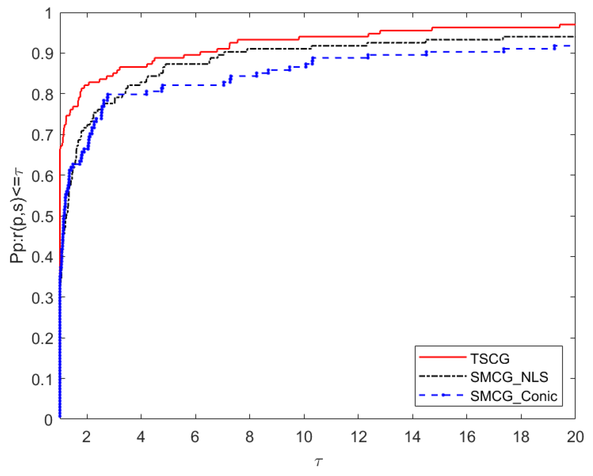
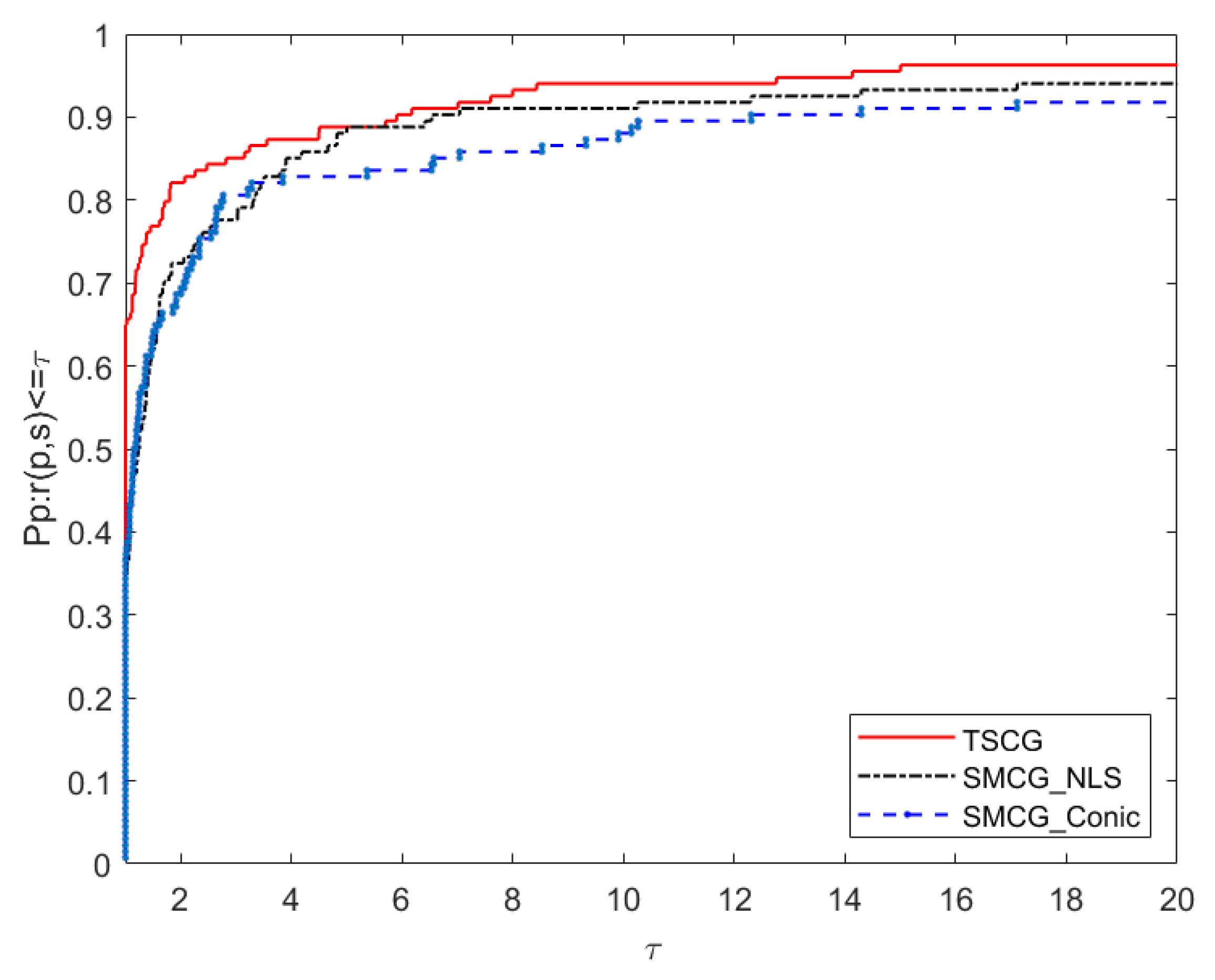
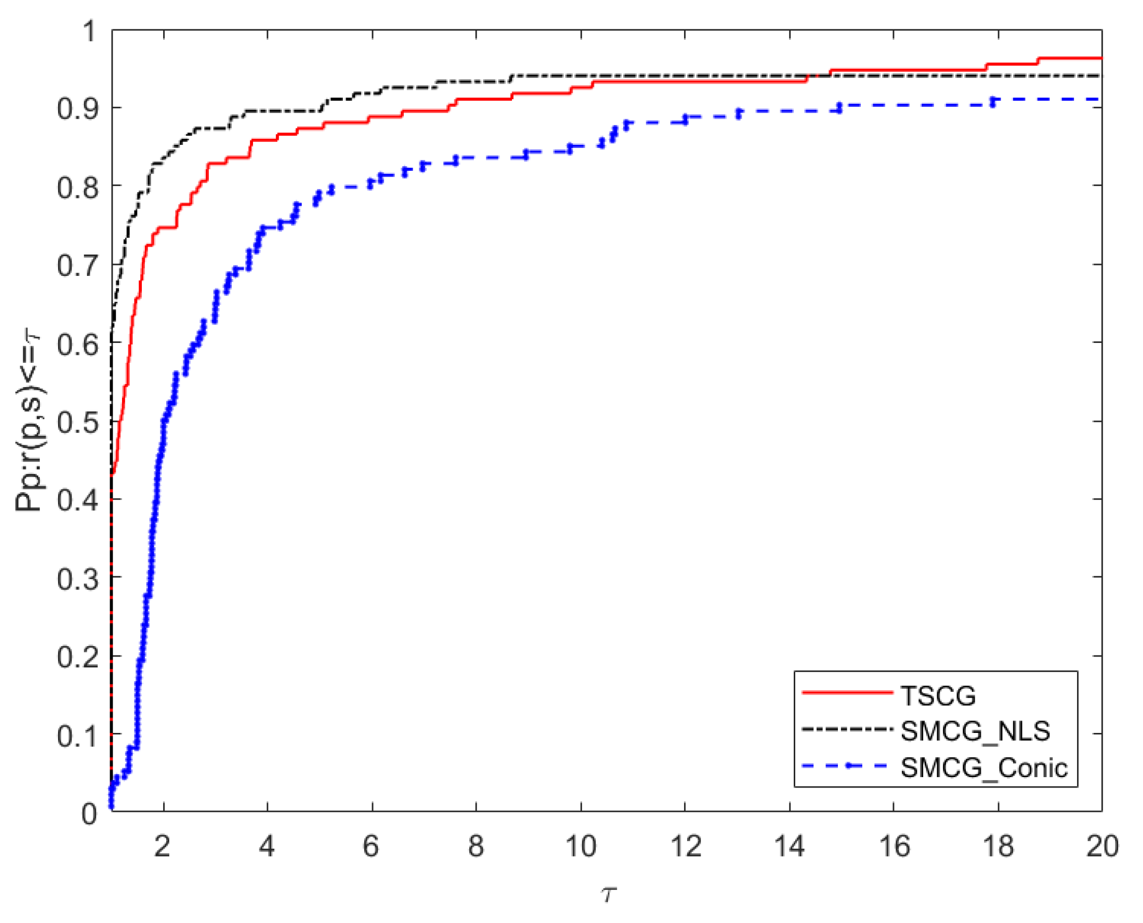
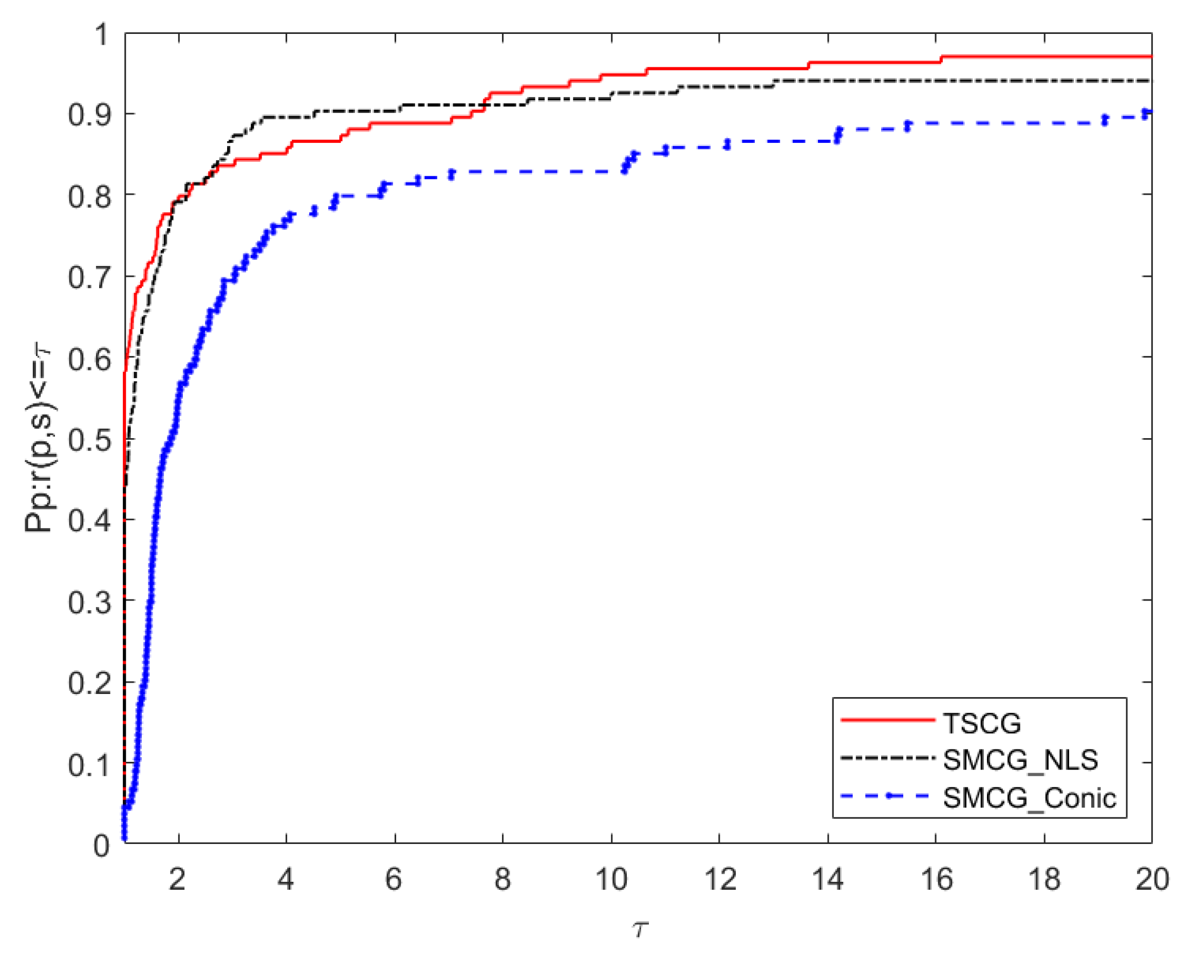
5. Numerical Results

In this section, we compare the numerical performance of the TSCG algorithm with SMCG_NLS [17] and SMCG_Conic [12] algorithms, both of which are subspace minimization algorithms, through numerical experiments to prove the effectiveness of the proposed TSCG algorithm. Performance profiles of Dolan and Moré [24] were used to test the performance of the method. Our test functions were derived from 67 functions in [25], as shown in

Table 1. The test problems.

No.	Test Problems	No.	Test Problems
1	Extended Freudenstein & Roth function	35	NONDIA function (CUTE)
2	Extended Trigonometric function	36	DQDRTIC function (CUTE)
3	Extended Rosenbrock function	37	EG2 function (CUTE)
4	Generalized Rosenbrock function	38	DIXMAANA - DIXMAANL functions
5	Extended White & Holst function	39	Partial Perturbed Quadratic function
6	Extended Beale function	40	Broyden Tridiagonal function
7	Extended Penalty function	41	Almost Perturbed Quadratic function
8	Perturbed Quadratic function	42	Perturbed Tridiagonal Quadratic function
9	Diagonal 1 function	43	Staircase 1 function
10	Diagonal 3 function	44	Staircase 2 function
11	Extended Tridiagonal 1 function	45	LIARWHD function (CUTE)
12	Full Hessian FH3 function	46	POWER function (CUTE)
13	Generalized Tridiagonal 2 function	47	ENGVAL1 function (CUTE)
14	Diagonal 5 function	48	CRAGGLVY function (CUTE)
15	Extended Himmelblau function	49	EDENSCH function (CUTE)
16	Generalized White & Holst function	50	CUBE function (CUTE)
17	Extended PSC1 function	51	BDEXP function (CUTE)
18	Extended Powell function	52	NONSCOMP function (CUTE)
19	Full Hessian FH2 function	53	VARDIM function (CUTE)
20	Extended Maratos function	54	SINQUAD function (CUTE)
21	Extended Cliff function	55	Extended DENSCHNB function (CUTE)
22	Perturbed quadratic diagonal function 2	56	Extended DENSCHNF function (CUTE)
23	Extended Wood function	57	LIARWHD function (CUTE)
24	Extended Hiebert function	58	COSINE function (CUTE)
25	Quadratic QF1 function	59	SINE function:83
26	Extended quadratic penalty QP1 function	60	Generalized Quartic function
27	Extended quadratic penalty QP2 function	61	Diagonal 7 function
28	Quadratic QF2 function	62	Diagonal 8 function
29	Extended quadratic exponential EP1 function	63	Extended TET function:(Three exponential terms)
30	Extended Tridiagonal 2 function	64	SINCOS function
31	FLETCHCR function (CUTE)	65	Diagonal 9 function
32	TRIDIA function (CUTE)	66	HIMMELBG function (CUTE)
33	ARGLINB function (CUTE)	67	HIMMELH function (CUTE)
34	ARWHEAD function (CUTE)

. It was programmed and run on a Windows 10 PC with a 1.80-GHz CPU and 16.00 GB memory, 64-bit operating system. We set the termination criteria as: $\parallel g_k\parallel \le \epsilon$, or when the number of iterations of the program exceeded 200,000, and exited when one of them was true. The dimensions of the variables of the test function were 10,000 and 12,000 respectively.

The following shows the selection of parameters and some tags and numerical experiments. The initial step size of the first iteration in this paper uses the adaptive strategy of [26].

$${\alpha }_0^{\left(0\right)}=\left\{\begin{array}{cc}1.0,\hfill & \mathrm{if}\parallel x_0{\parallel }_{\infty }<{10}^{-30}and{\parallel f_0\parallel }_{\infty }<{10}^{-30},\hfill \\ 2\frac{|f_0|}{\parallel g_0\parallel },\hfill & \mathrm{if}\parallel x_0{\parallel }_{\infty }<{10}^{-30}and{\parallel f_0\parallel }_{\infty }\ge {10}^{-30},\hfill \\ min\left\{1.0,\frac{\parallel x_0{\parallel }_{\infty }}{\parallel g_0{\parallel }_{\infty }}\right\},\hfill & \mathrm{if}\parallel x_0{\parallel }_{\infty }\ge {10}^{-30}and{\parallel g_0\parallel }_{\infty }<{10}^7,\hfill \\ min\left\{1.0,max\left\{\frac{\parallel x_0{\parallel }_{\infty }}{\parallel g_0{\parallel }_{\infty }},\frac{1}{\parallel g_0{\parallel }_{\infty }}\right\}\right\},\hfill & \mathrm{if}\parallel x_0{\parallel }_{\infty }\ge {10}^{-30}and{\parallel g_0\parallel }_{\infty }\ge {10}^7,\hfill \end{array}\right.$$

where ${\parallel ·\parallel }_{\infty }$ represents the infinite norm.

The parameters of SMCG_NLS and SMCG_Conic algorithms are selected according to the values selected in the original paper. The parameters of the TSCG algorithm proposed by us are selected as follows.

$\epsilon ={10}^{-6},\delta =0.001,\sigma =0.9999,{\xi }_1={10}^{-7},{\xi }_2={10}^6,{\xi }_3={10}^{-4},{\xi }_4=0.875,$

${\xi }_5={10}^{-8},{\xi }_6={10}^{-12},{\lambda }_1={10}^{-5},{\lambda }_2=0.06,{\vartheta }_{min}={10}^{-30},{\vartheta }_{max}={10}^{30}.$

The relevant tags of this article are as follows:

• Ni: the number of iterations.
• Nf: the number of function evaluations.
• Ng: the number of gradient evaluations.
• CPU: the running time of the algorithm (in seconds).

Now, we compare the algorithm TSCG in this paper with SMCG_NLS [17] and SMCG_Conic [12] in numerical diagrams. The performance comparison diagrams of Ni, Ng, Nf and CPU correspond to Figure 1, Figure 2, Figure 3 and Figure 4 respectively. According to Figure 1 and Figure 2, it is found that the robustness and stability of TSCG are significantly better than that of SMCG_NLS and SMCG_Conic in terms of the number of iterations and the total number of gradient calculations. Overall, SMCG_NLS has better robustness and stability than SMCG_Conic. From Figure 3, we know that both TSCG and SMCG_NLS are superior to SMCG_Conic, and TSCG begins to be better than SMCG_NLS when $\tau \ge 14.3231$, even when factor $\tau \le 14.3231$, the total calculated by the function TSCG does not perform as well as SMCG_NLS. Figure 4 shows that TSCG and SMCG_NLS are better than SMCG_Conic in terms of the robustness and stability of running time. In general, TSCG is almost better than SMCG_NLS in terms of robustness and stability, only when factor $2.6328\le \tau \le 7.6472$, TSCG is inferior to SMCG_NLS.

6. Conclusions and Prospect

In order to obtain a more efficient and robust conjugate gradient algorithm for solving the unconstrained optimization problem, by constructing a new three-dimensional subspace ${\Omega }_{k+1}=Span\{g_{k+1},s_k,y_k^{*}\}$, and solving the sub-problem of a quadratic approximate model of the objective function in the given subspace, we obtained a new three-term conjugate gradient method (TSCG). The global convergence of the TSCG method for general functions is established under mild conditions. Numerical results show that TSCG has better performance than SMCG_NLS and SMCG_Conic, both of which are subspace algorithms, for a given test set.

As for the research of the subspace algorithm, the main content of our future work is to continue to study the estimation of terms, including Hessian matrix, to discuss whether it can be extended to the constrained optimization algorithm, and consider the application of the algorithm to image restoration, image segmentation, and path planning of engineering problems.

References

1. Hestenes, M.R.; Stiefel, E. Methods of conjugate gradients for solving linear systems. J. Res. Natl. Bur. Stand. 1952, 49, 409–436. [Google Scholar] [CrossRef]
2. Fletcher, R.; Reeves, C.M. Function minimization by conjugate gradients. Comput. J. 1964, 7, 149–154. [Google Scholar] [CrossRef] [Green Version]
3. Polyak, B.T. The conjugate gradient method in extremal problems. JUssr Comput. Math. Math. Phys. 1969, 9, 94–112. [Google Scholar] [CrossRef]
4. Liu, Y.; Storey, C. Efficient generalized conjugate gradient algorithms, part 1: Theory. J. Optim. Theory Appl. 1991, 69, 129–137. [Google Scholar] [CrossRef]
5. Dai, Y.H.; Yuan, Y. A nonlinear conjugate gradient method with a strong global convergence property. Siam J. Optim. 1999, 10, 177–182. [Google Scholar] [CrossRef] [Green Version]
6. Fletcher, R. Volume 1 Unconstrained Optimization. In Practical Methods of Optimization; Wiley-Interscience: New York, NY, USA, 1980; p. 120. [Google Scholar]
7. Zhang, H.; Hager, W.W. A non-monotone line search technique and its application to unconstrained optimization. Soc. Ind. Appl. Math. J. Optim. 2004, 14, 1043–1056. [Google Scholar]
8. Liu, H.; Liu, Z. An efficient Barzilai–Borwein conjugate gradient method for unconstrained optimization. J. Optim. Theory Appl. 2019, 180, 879–906. [Google Scholar] [CrossRef]
9. Yuan, Y.X.; Stoer, J. A subspace study on conjugate gradient algorithms. ZAMM-J. Appl. Math. Mech. FüR Angew. Math. Und Mech. 1995, 75, 69–77. [Google Scholar] [CrossRef]
10. Dai, Y.H.; Kou, C.X. A Barzilai–Borwein conjugate gradient method. Sci. China Math. 2016, 59, 1511–1524. [Google Scholar] [CrossRef]
11. Barzilai, J.; Borwein, J.M. Two-Point Step Size Gradient Methods. IMA J. Numer. Anal. 1988, 8, 141–148. [Google Scholar] [CrossRef]
12. Li, Y.; Liu, Z.; Hongwei, L. A subspace minimization conjugate gradient method based on conic model for unconstrained optimization. Comput. Appl. Math. 2019, 38, 16. [Google Scholar] [CrossRef]
13. Wang, T.; Liu, Z.; Liu, H. A new subspace minimization conjugate gradient method based on tensor model for unconstrained optimization. Int. J. Comput. Math. 2019, 96, 1924–1942. [Google Scholar] [CrossRef]
14. Zhao, T.; Liu, H.; Liu, Z. New subspace minimization conjugate gradient methods based on regularization model for unconstrained optimization. Numer. Algorithms 2020, 87, 1501–1534. [Google Scholar] [CrossRef]
15. Andrei, N. An accelerated subspace minimization three-term conjugate gradient algorithm for unconstrained optimization. Numer. Algorithms 2014, 65, 859–874. [Google Scholar] [CrossRef]
16. Yang, Y.; Chen, Y.; Lu, Y. A subspace conjugate gradient algorithm for large-scale unconstrained optimization. Numer. Algorithms 2017, 76, 813–828. [Google Scholar] [CrossRef]
17. Li, M.; Liu, H.; Liu, Z. A new subspace minimization conjugate gradient method with non-monotone line search for unconstrained optimization. Numer. Algorithms 2018, 79, 195–219. [Google Scholar] [CrossRef]
18. Yao, S.; Wu, Y.; Yang, J.; Xu, J. A Three-Term Gradient Descent Method with Subspace Techniques. Math. Probl. Eng. 2021, 2021, 8867309. [Google Scholar] [CrossRef]
19. Yuan, Y. A review on subspace methods for nonlinear optimization. Proc. Int. Congr. Math. 2014, 807–827. [Google Scholar]
20. Wei, Z.; Yao, S.; Liu, L. The convergence properties of some new conjugate gradient methods. Appl. Math. Comput. 2006, 183, 1341–1350. [Google Scholar] [CrossRef]
21. Yuan, Y. A modified BFGS algorithm for unconstrained optimization. IMA J. Numer. Anal. 1991, 11, 325–332. [Google Scholar] [CrossRef]
22. Dai, Y.; Yuan, J.; Yuan, Y.X. Modified two-point stepsize gradient methods for unconstrained optimization. Comput. Optim. Appl. 2002, 22, 103–109. [Google Scholar] [CrossRef]
23. Dai, Y.H.; Kou, C.X. A nonlinear conjugate gradient algorithm with an optimal property and an improved Wolfe line search. Soc. Ind. Appl. Math. J. Optim. 2013, 23, 296–320. [Google Scholar] [CrossRef] [Green Version]
24. Dolan, E.D.; Moré, J.J. Benchmarking optimization software with performance profiles. Math. Program. 2002, 91, 201–213. [Google Scholar] [CrossRef]
25. Andrei, N. An unconstrained optimization test functions collection. Adv. Model. Optim. 2008, 10, 147–161. [Google Scholar]
26. Hager, W.W.; Zhang, H. A new conjugate gradient method with guaranteed descent and an efficient line search. SIAM J. Optim. 2005, 16, 170–192. [Google Scholar] [CrossRef] [Green Version]
Figure 1. Performance profiles of the number of iterations (Ni).
Symmetry 14 00080 g001
Figure 2. Performance profiles of the gradient (Ng).
Symmetry 14 00080 g002
Figure 3. Performance profiles of the function (Nf).
Symmetry 14 00080 g003
Figure 4. Performance profiles of CPU time (CPU).
Symmetry 14 00080 g004