Lie Group Classification of Generalized Variable Coefficient Korteweg-de Vries Equation with Dual Power-Law Nonlinearities with Linear Damping and Dispersion in Quantum Field Theory

Abstract

Many physical phenomena in fields of studies such as optical fibre, solid-state physics, quantum field theory and so on are represented using nonlinear evolution equations with variable coefficients due to the fact that the majority of nonlinear conditions involve variable coefficients. In consequence, this article presents a complete Lie group analysis of a generalized variable coefficient damped wave equation in quantum field theory with time-dependent coefficients having dual power-law nonlinearities. Lie group classification of two distinct cases of the equation was performed to obtain its kernel algebra. Thereafter, symmetry reductions and invariant solutions of the equation were obtained. We also investigate various soliton solutions and their dynamical wave behaviours. Further, each class of general solutions found is invoked to construct conserved quantities for the equation with damping term via direct technique and homotopy formula. In addition, Noether’s theorem is engaged to furnish more conserved currents of the equation under some classifications.

1. Introduction

The far-famed Korteweg-de Vrie (KdV) equation

$$u_t-6u{u}_x+u_{xxx}=0,$$

(1)

which is a dispersive nonlinear evolution Equation (NLEVEQ) is a mathematical model which delineates the special waves referred to as soliton on shallow water surface [1]. The KdV equation is interconnected in diverse ways to physical problems that involve acoustic waves on a crystal lattice as well as ion-acoustic waves in a plasma, long internal waves in a density-stratified ocean along with shallow water waves with weakly non-linear restoring forces.

Nonlinearity is a captivating and enthralling element of nature. Besides, it is a known fact that many physical phenomena are represented by NLEVEQ as well as its higher-order form with variable coefficients because the vast majority of genuine nonlinear physical conditions involve variable coefficients. Scientists in their numbers have deemed it fit to contemplate nonlinear science as the most significant frontier for the fundamental comprehension of nature. Some of these models include a generalized system of three dimensional variable-coefficient modified Kadomtsev–Petviashvili–Burgers-type equation in [2] was studied. The modified and generalized Zakharov–Kuznetsov model, which recounts the ion-acoustic drift solitary waves existing in a magnetoplasma with electron-positron-ion which are found in the primordial universe was investigated in [3,4]. This equation was used to model ion-acoustic, dust-magneto-acoustic, quantum-dust-ion-acoustic and/or dust-ion-acoustic waves in one of the cosmic or laboratory dusty plasmas. Moreover, in [5] the vector bright solitons, as well as their interaction characteristics of the coupled Fokas–Lenells system, which models the femtosecond optical pulses in a birefringent optical fibre, was examined. In addition, the Boussinesq–Burgers-type system of equations which delineates shallow water waves appearing close to lakes or ocean beaches was studied in [6], to name a few, see more in [7,8,9,10].

Lie group theory was brought to light by a Norwegian mathematician whose name was Marius Sophus Lie (1842–1899). This occurred around the middle of the nineteenth century. Lie, in their research recognized that the seemingly dissimilar techniques for securing exact solutions of differential equations (DEQs) were, in fact, all special cases of a wide integration approach; the theory of transformation groups. Analogous to this theory is the Galois theory which has an enormous influence on mathematics and mathematical physics today. In fact to be precise, the origins of Lie group are to be found in Galois’ simple, yet profound observation that the set of symmetries of a geometric object forms a group. Through a surprisingly tortuous route that began with a study of the integration of partial differential equations (PDEQs), Lie was led to introduce the continuous groups that now bear their name, an accomplishment that has had remarkable consequences for mathematics and physics. In addition, Lie often viewed their mission particularly as the extension of Galois theory to the study of differential equations [11].

Further, it is regarded to be one of the most pertinent and significant techniques for determining closed-form solutions of differential equations. Lie symmetry analysis [11,12,13,14,15,16] has been given some credits in light of the fact that it is one of the most efficient techniques engaged in the analysis of differential equations. The last few decades have witnessed a long overdue and widespread popularization of Lie’s constructive, infinitesimal symmetry methods, applied to an incredible variety of mathematical, physical and other problems. Less well documented though, is the role symmetry groups play in the classification of differential equations and variational problems. Of particular importance is Lie’s classification of all possible Lie groups of transformations acting on one-dimensional as well as two-dimensional manifolds. The symmetry groups that arise most often in the applications to geometry and differential equations are Lie groups of transformations acting on a finite-dimensional manifolds [11].

There are many studies in the literature dealing with the analysis of differential equations based on Lie symmetries, reductions and invariant solutions [3,4,17].

In addition to Lie symmetry analysis and inverse scattering transform [18] which was developed to find solutions to the KdV equation, many other essential approaches for achieving closed-form solution of NLEVEQ have been given. These comprise exp$(-\mathsf{\Phi }(\eta ))$-expansion technique [19,20], Painlevé expansion [21], Cole–Hopf transformation approach [22], Adomian decomposition approach [23], homotopy perturbation technique [24], mapping method and extended mapping method [25,26], Bäcklund transformation [27], rational expansion method [28], F-expansion technique [29], tan-cot method [30], extended simplest equation method [31], Hirota technique [32], bifurcation technique [33] and so on.

One of the ways by which physical systems are studied is the consideration of the generalized structure of the model representing these systems [3]. An example is the KdV equation with dual-power law nonlinearity presented as [34]

$$u_t+p{u}^n{u}_x+q{u}^{2n}{u}_x+r{u}_{xxx}=0,$$

(2)

with nonzero constant coefficients p, q and r. Equation (2) possesses various applications with regards to quantum field theory, plasma as well as solid-state physics [34]. For instance, the kink soliton can be utilized in calculating momentum, energy flow along with the topological charge in the quantum field. Particular cases $n=1$ and $n=2$ which we call KdV and modified KdV equations, respectively, have been studied by researchers. For example, Dey and Coffey [35,36] investigated the kink-profile solitary wave solutions of (2). Generalized Equation (2) was investigated recently by the authors in [37] where they secured the general analytic travelling wave solutions of the equation as dark, bright as well as periodic soliton solutions. These general solutions were achieved for different values of parameter n.

Mathematical Analysis

We investigate Lie group classification of two different cases of the generalized variable coefficient KdV equation with dual power-law nonlinearities and linear damping dispersion ((1+1)D-gvcKdVDampe) in quantum field theory which is expressed as:

$$u_t+Q(t)u^n{u}_x+S(t)u^{2m}{u}_x+H(t)u+G(t)u_{xxx}=0$$

(3)

with time-variable coefficients $Q(t)$, $S(t)$, $H(t)$ and $G(t)$ together with positive integer exponents n and m. In Equation (3), $u_t$ which is the first term represents the evolution term while the second term is referred to as the power law nonlinearity with n called the index of power law. Besides, the third term is the dual power law nonlinearity where $2m$ is the index of dual power law while $H(t)u$ depicts linear damping term and $G(t)u_{xxx}$ denotes the dispersion term.

Equation (3) is a more generalized version of the KdV equation with power law nonlinearity with linear damping and dispersion which reads [38]:

$$u_t+a(t)u^n{u}_x-l(t)u_x-b(t)u+c(t)u_{xxx}=0$$

(4)

where $a(t)$, $b(t)$, $c(t)$ and $l(t)$ are arbitrary smooth functions with regards to t. A special case of (4) with $a(t)=6,n=1$, $b(t)=0$, $c(t)=1$ and $l(t)=-1/2t$ was examined in [38]. The authors implored Lie symmetry analysis to secure optimal system together with invariant solutions of the equation under the given case. In [39], the author via the ansatz technique, gained some exact solitary wave solutions of the equation with power law nonlinearity with time-dependent coefficients of the nonlinear alongside the dispersion terms. These solutions were secured with regards to tan-hyperbolic as well as cos-hyperbolic functions. Moreover Johnpillai et al. [40] investigated Lie point symmetries and exact solutions of the modified structure of (4) with time-dependent coefficients taking into consideration special cases $a(t)=1/t$, $c(t)=K/t^2$ as well as $a(t)=K_0$, $c(t)=K_{1}exp(-2K_{0}t)$ where K, $K_0$ and $K_1$ are regarded as constants. In consequence, diverse bright soliton, dark soliton and singular soliton wave solutions were secured via ansatz approach. Further, the authors in [41] have studied Lie symmetry classification of the version of KdV equation.

In the literature, Vaneeva [42] studied the variable-coefficient Gardner equation

$$u_t+A_2(t)u{u}_x+A_3(t)u^2{u}_x+A_1(t)u_{xxx}=0,$$

(5)

with $A_2(t)$ together with $A_3(t)$, smooth functions satisfying the condition that $A_1(t).A_3(t)\ne 0$. Moreover, Bruzon et al. [43] investigated generalized Gardner equation structured as:

$$u_t+A_2(t)u^n{u}_x+A_3(t)u^{2n}{u}_x+A_1(t)u_{xxx}+A_4(t)u=0,$$

(6)

where positive integer n is arbitrary. Besides, Lie point symmetries alongside conservation laws of the equation for $n=1$ are further examined in [44]. A version of generalized variable-coefficient Gardner Equation (6) of the form [45]:

$$u_t+A_2(t)u^m{u}_x+A_3(t)u^{2n}{u}_x+A_1(t)u_{xxx}+A_4(t)u=0,$$

(7)

with positive integer m was investigated. The authors obtained $\mu$-symmetries, $\mu$-invariant and $\mu$-conservation laws of the equation. It is to be observed that the generalized version of (4) contemplated in this study in a way resembles (7). However, techniques utilized are not exactly the same and as such completely different results are obtained.

In this research work, we catalogue our article in the structure given subsequently, that is, in Section 2, we carry out Lie group classification of (1+1)D-gvcKdVDampe (3) for cases $H(t)\ne 0$ and $H(t)=0$ when $n=m$ using the appropriate equivalence transformations. In addition, we obtained adequate extended Lie algebras under each classification, perform symmetry reductions and obtained invariant solutions. We further study various soliton solutions of the equation and their dynamical wave behaviours which are later analyzed. Section 3 investigates Lie group analysis of the underlying equation for $n\ne m$. Section 4 purveys various observations and discussion of the obtained results. Further, in Section 5, we give the various graphical depictions of the results obtained and discuss them. Section 6 purveys the conservation laws of the underlying equation with the use of the multiplier technique. Noether’s theorem is also invoked to achieve more conserved currents of the equation. Later, we give the concluding remarks in Section 7.

2. Lie Group Classification of (3) When $\mathit{n}\mathbf{=}\mathit{m}$

We first contemplate the Lie group classification of variable coeffcient (1+1)D-gvcKdV-Dampe (3) when $n=m$ in this section.

2.1. Equivalence Transformations

We seek equivalence transformation of class (3) and in making a success of that we recollect that an equivalence transformation regarding a partial differential Equation (PDEQ) refers to an invertible transformation of both the independent as well as dependent variables mapping the PDEQ into another PDEQ possessing the same structure, where the structure assumed by the transformed functions can, in general, vary from the structure of the original function. In other words, an equivalence transformation of class (3) in this instance depicts a non-degenerating point transformation $(t,x,u(t,x))$ to $(\tilde{t},\tilde{x},\tilde{u}(\tilde{t},\tilde{x}))$ that retains differential form but with different arbitrary functions $\tilde{Q}(\tilde{t})$, $\tilde{S}(\tilde{t})$, $\tilde{G}(\tilde{t})$ and $\tilde{H}(\tilde{t})$ from the original one. In consequence, we present equivalence transformations of (3) in the subsequent subsection.

2.2. Case 1. $H(t)\ne 0$

We contemplate the one-parameter group of equivalence transformations that is in $(t,x,u,Q,S,G,H)$ related to (3) where we have $H(t)\ne 0$ and that is defined by:

$$\begin{array}{cc}\hfill & \tilde{t}=t+ϵ{\xi }^1(t,x,u)+O({ϵ}^2),\hfill \\ \hfill & \tilde{x}=x+ϵ{\xi }^2(t,x,u)+O({ϵ}^2),\hfill \\ \hfill & \tilde{u}=u+ϵ\eta (t,x,u)+O({ϵ}^2),\hfill \\ \hfill & \tilde{Q}=Q+ϵ{\mathsf{\Omega }}^1(t,x,u,Q,S,G,H)+O({ϵ}^2),\hfill \\ \hfill & \tilde{S}=S+ϵ{\mathsf{\Omega }}^2(t,x,u,Q,S,G,H)+O({ϵ}^2),\hfill \\ \hfill & \tilde{G}=G+ϵ{\mathsf{\Omega }}^3(t,x,u,Q,S,G,H)+O({ϵ}^2),\hfill \\ \hfill & \tilde{H}=H+ϵ{\mathsf{\Omega }}^4(t,x,u,Q,S,G,H)+O({ϵ}^2),\hfill \end{array}$$

where $ϵ$ represents the group parameter. Therefore, the operator given as:

$$\begin{array}{c}\hfill \mathcal{Q}={\xi }^1{\partial }_t+{\xi }^2{\partial }_x+\eta {\partial }_u+{\mathsf{\Omega }}^1{\partial }_Q+{\mathsf{\Omega }}^2{\partial }_S+{\mathsf{\Omega }}^3{\partial }_G+{\mathsf{\Omega }}^4{\partial }_H,\end{array}$$

(8)

is defined as the generator of the equivalence group for (3) provided that the same is admitted by the extended system expressed as:

$$\begin{array}{c}\hfill u_t+Q(t)u^n{u}_x+S(t)u^{2n}{u}_x+H(t)u+G(t)u_{xxx}=0,\\ \hfill Q_x=Q_u=S_x=S_u=G_x=G_u=H_x=H_u=0.\end{array}$$

(9)

Now, the prolonged operator for the given extended system (9) has the structure:

$$\begin{array}{cc}\hfill \tilde{\mathcal{Q}}=& \mathcal{Q}+{\zeta }_t{\partial }_{u_t}+{\zeta }_x{\partial }_{u_x}+{\zeta }_{xxx}{\partial }_{u_{xxx}}+{\mu }_x^1{\partial }_{Q_x}+{\mu }_u^1{\partial }_{Q_u}+{\mu }_x^2{\partial }_{S_x}+{\mu }_u^2{\partial }_{S_u}\hfill \\ & +{\mu }_x^3{\partial }_{G_x}+{\mu }_u^3{\partial }_{G_u}+{\mu }_x^4{\partial }_{H_x}+{\mu }_u^4{\partial }_{H_u}.\hfill \end{array}$$

(10)

We define the variables $\zeta$’s and $\mu$’s in (10) via the prolongation relation:

$$\begin{array}{cc}\hfill & {\zeta }_t=D_t(\eta )-u_t{D}_t({\xi }^1)-u_x{D}_t({\xi }^2),\hfill \\ \hfill & {\zeta }_x=D_x(\eta )-u_t{D}_x({\xi }^1)-u_x{D}_x({\xi }^2),\hfill \\ \hfill & {\zeta }_{xx}=D_x({\zeta }_x)-u_{tx}{D}_x({\xi }^1)-u_{xx}{D}_x({\xi }^2),\hfill \\ \hfill & {\zeta }_{xxx}=D_x({\zeta }_{xx})-u_{txx}{D}_x({\xi }^1)-u_{xxx}{D}_x({\xi }^2)\hfill \end{array}$$

along with:

$$\begin{array}{cc}\hfill & {\mu }_x^1={\tilde{D}}_x({\mathsf{\Omega }}^1)-Q_t{\tilde{D}}_x({\xi }^1)-Q_x{\tilde{D}}_x({\xi }^2)-Q_u{\tilde{D}}_x(\eta ),\hfill \\ \hfill & {\mu }_u^1={\tilde{D}}_u({\mathsf{\Omega }}^1)-Q_t{\tilde{D}}_u({\xi }^1)-Q_x{\tilde{D}}_u({\xi }^2)-Q_u{\tilde{D}}_u(\eta ),\hfill \\ \hfill & {\mu }_x^2={\tilde{D}}_x({\mathsf{\Omega }}^2)-S_t{\tilde{D}}_x({\xi }^1)-S_x{\tilde{D}}_x({\xi }^2)-S_u{\tilde{D}}_x(\eta ),\hfill \\ \hfill & {\mu }_u^2={\tilde{D}}_u({\mathsf{\Omega }}^2)-S_t{\tilde{D}}_u({\xi }^1)-S_x{\tilde{D}}_u({\xi }^2)-S_u{\tilde{D}}_u(\eta ),\hfill \\ \hfill & {\mu }_x^3={\tilde{D}}_x({\mathsf{\Omega }}^3)-G_t{\tilde{D}}_x({\xi }^1)-G_x{\tilde{D}}_x({\xi }^2)-G_u{\tilde{D}}_x(\eta ),\hfill \\ \hfill & {\mu }_u^3={\tilde{D}}_u({\mathsf{\Omega }}^3)-G_t{\tilde{D}}_u({\xi }^1)-G_x{\tilde{D}}_u({\xi }^2)-G_u{\tilde{D}}_u(\eta ),\hfill \\ \hfill & {\mu }_x^4={\tilde{D}}_x({\mathsf{\Omega }}^4)-H_t{\tilde{D}}_x({\xi }^1)-H_x{\tilde{D}}_x({\xi }^2)-H_u{\tilde{D}}_x(\eta ),\hfill \\ \hfill & {\mu }_u^4={\tilde{D}}_u({\mathsf{\Omega }}^4)-H_t{\tilde{D}}_u({\xi }^1)-H_x{\tilde{D}}_u({\xi }^2)-H_u{\tilde{D}}_u(\eta ),\hfill \end{array}$$

where we have accordingly,

$$\begin{array}{c}\hfill D_t=\frac{\partial }{\partial t}+u_t\frac{\partial }{\partial u}+\cdots ,D_x=\frac{\partial }{\partial x}+u_x\frac{\partial }{\partial u}+\cdots \end{array}$$

(11)

as the total derivative operators. In addition, we also have:

$$\begin{array}{cc}\hfill & {\tilde{D}}_x=\frac{\partial }{\partial x}+Q_x\frac{\partial }{\partial Q}+S_x\frac{\partial }{\partial S}+G_x\frac{\partial }{\partial G}+H_x\frac{\partial }{\partial H}+\cdots ,\hfill \\ \hfill & {\tilde{D}}_u=\frac{\partial }{\partial u}+Q_u\frac{\partial }{\partial Q}+S_u\frac{\partial }{\partial S}+G_u\frac{\partial }{\partial G}+H_u\frac{\partial }{\partial H}+\cdots \hfill \end{array}$$

presented as the total derivative operators of the extended system expressed in (9). Application of (10) to the extended system (9) and thereafter splitting the outcome on derivatives of u, one achieves overdetermined system of linear partial differential equations which are secured as:

$$\begin{array}{cc}\hfill & {\xi }_x^1={\xi }_u^1=0,{\mathsf{\Omega }}_x^1={\mathsf{\Omega }}_u^1={\mathsf{\Omega }}_x^2={\mathsf{\Omega }}_u^2={\mathsf{\Omega }}_x^3={\mathsf{\Omega }}_u^3={\mathsf{\Omega }}_x^4={\mathsf{\Omega }}_u^4=0,\hfill \\ \hfill & {\xi }_u^2=0,{\eta }_{uu}=0,{\eta }_{xu}-{\xi }_{xx}^2=0,{\mathsf{\Omega }}^3+({\xi }_t^1-3{\xi }_x^2)G=0,\hfill \\ \hfill & {\eta }_t+{\eta }_x\left(Q{u}^n+S{u}^{2n}\right)+G{\eta }_{xxx}+H\eta +{\mathsf{\Omega }}^{4}u=0,\hfill \\ \hfill & {\mathsf{\Omega }}^1{u}^n+{\mathsf{\Omega }}^2{u}^{2n}+nQ{u}^{n-1}\eta +2nS{u}^{2n-1}\eta -{\xi }_t^2-G{\xi }_{xxx}^2\hfill \\ \hfill & +3G{\eta }_{xxu}+({\xi }_t^1-{\xi }_x^2)\left(Q{u}^n+S{u}^{2n}\right)=0.\hfill \end{array}$$

(12)

On solving the obtained system of equations given in (12) we achieve:

$$\begin{array}{cc}\hfill & {\xi }^1=a(t),\hfill \\ \hfill & {\xi }^2=A_{1}x+A_2,\hfill \\ \hfill & \eta =b(t)u,\hfill \\ \hfill & {\mathsf{\Omega }}^1=\left(A_1-a^{\prime }(t)-nb(t)\right)Q,\hfill \\ \hfill & {\mathsf{\Omega }}^2=(A_1-a^{\prime }(t)-2nb(t))S,\hfill \\ \hfill & {\mathsf{\Omega }}^3=(3A_1-a^{\prime }(t))G,\hfill \\ \hfill & {\mathsf{\Omega }}^4=-(b^{\prime }(t)+b(t)H),\hfill \end{array}$$

where $A_1$ and $A_2$ are constants as well as $a(t)$ and $b(t)$ arbitrary functions of t. As a result, the equivalence generators of class (3) are calculated as:

$$\begin{array}{cc}\hfill & {\mathcal{Q}}_1={\partial }_x,\hfill \\ \hfill & {\mathcal{Q}}_2=x{\partial }_x+Q{\partial }_Q+S{\partial }_S+3G{\partial }_G,\hfill \\ \hfill & {\mathcal{Q}}_a=a(t){\partial }_t-a^{\prime }(t)Q{\partial }_Q-a^{\prime }(t)S{\partial }_S-a^{\prime }(t)G{\partial }_G,\hfill \\ \hfill & {\mathcal{Q}}_b=b(t)u{\partial }_u-nb(t)Q{\partial }_Q-2nb(t)S{\partial }_S-\left(b^{\prime }(t)+b(t)H\right){\partial }_H.\hfill \end{array}$$

Correspondingly, the equivalence group associated to each of the equivalence generators is presented as:

$$\begin{array}{cc}\hfill & {\mathcal{Q}}_1:\tilde{t}=t,\tilde{x}=x+c_1,\tilde{u}=u,\tilde{Q}=Q,\tilde{S}=S,\tilde{G}=G,\tilde{H}=H,\hfill \\ \hfill & {\mathcal{Q}}_2:\tilde{t}=t,\tilde{x}=x{e}^{c_2},\tilde{u}=u,\tilde{Q}=Q{e}^{c_2},\tilde{S}=S{e}^{c_2},\tilde{G}=G{e}^{3c_2},\tilde{H}=H,\hfill \\ \hfill & {\mathcal{Q}}_a:\tilde{t}=a(t),\tilde{x}=x,\tilde{u}=u,\tilde{Q}=\frac{Q}{a^{\prime }(t)},\tilde{S}=\frac{S}{a^{\prime }(t)},\tilde{G}=\frac{G}{a^{\prime }(t)},\tilde{H}=H,\hfill \\ \hfill & {\mathcal{Q}}_b:\tilde{t}=t,\tilde{x}=x,\tilde{u}=u{e}^{b(t)c_4},\tilde{Q}=Q{e}^{-nb(t)c_4},\tilde{S}=S{e}^{-2nb(t)c_4},\tilde{G}=G,\hfill \\ \hfill & \tilde{H}=H{e}^{-b(t)c_4}-b^{\prime }(t)c_4.\hfill \end{array}$$

Moreover, the composition of ${\mathcal{Q}}_1,\dots ,{\mathcal{Q}}_b$, when computed produces:

$$\begin{array}{cc}\hfill & \tilde{t}=a(t),\tilde{x}=\left(x+c_1\right)e^{c_2},\tilde{u}=u{e}^{b(t)c_4},\tilde{Q}=\frac{Q{e}^{c_2-nb(t)c_4}}{a^{\prime }(t)},\hfill \\ \hfill & \tilde{S}=\frac{S{e}^{c_2-2nb(t)c_4}}{a^{\prime }(t)},\tilde{G}=\frac{G{e}^{3c_2}}{a^{\prime }(t)},\tilde{H}=H{e}^{-b(t)c_4}-b^{\prime }(t)c_4.\hfill \end{array}$$

(13)

Further, since we are having two arbitrary functions $a(t)$ alongside $b(t)$ in (13), it is observed that one can rescale two of the arbitrary functions which are present in (3) [42,46]. Therefore, we set $\tilde{G}=\tilde{H}=1$ and in consequence, we achieve:

$$a(t)=\int Q{e}^{3c_2}dt,b(t)=\frac{1}{c_4}\left\{ln\left(c_4+c_4\int H{e}^{t{c}_4}dt\right)-t{c}_4\right\}$$

(14)

and so we eventually have the equivalence transformation:

$$\begin{array}{c}\hfill \tilde{t}=\int G{e}^{3c_2}dt,\tilde{x}=\left(x+c_1\right)e^{c_2},\tilde{u}=u{c}_4{e}^{-t{c}_4}\int H{e}^{t{c}_4}dt,\end{array}$$

(15)

which by extension transforms (3) into an equivalent equation expressed as:

$$\begin{array}{c}\hfill {\tilde{u}}_{\tilde{t}}+\tilde{Q}(\tilde{t}){\tilde{u}}^{\tilde{n}}{\tilde{u}}_{\tilde{x}}+\tilde{S}(\tilde{t}){\tilde{u}}^{2\tilde{n}}{\tilde{u}}_{\tilde{x}}+\tilde{u}+{\tilde{u}}_{\tilde{x}\tilde{x}\tilde{x}}=0,\end{array}$$

where

$$\begin{array}{c}\hfill \tilde{Q}=\frac{Q{e}^{-(nb(t)c_4+2c_2)}}{G},\tilde{S}=\frac{S{e}^{-2(nb(t)c_4+c_2)}}{G}.\end{array}$$

Hence, without loss of generality, we can restrict our investigation to the equation

$$\begin{array}{c}\hfill u_t+Q(t)u^n{u}_x+S(t)u^{2n}{u}_x+u+u_{xxx}=0.\end{array}$$

(16)

2.3. Case 2. $H(t)=0$

In this case, Equation (3) narrows down to a time variable-coefficient version of the well celebrated KdV equation, which implies

$$u_t+Q(t)u^n{u}_x+S(t)u^{2n}{u}_x+G(t)u_{xxx}=0.$$

(17)

On invoking the appropriate steps in solving the related extended system to (17) as we have earlier demonstrated we secure the system of equations calculated as:

$$\begin{array}{cc}\hfill & {\xi }_x^1={\xi }_u^1=0,{\mathsf{\Omega }}_x^1={\mathsf{\Omega }}_u^1={\mathsf{\Omega }}_x^2={\mathsf{\Omega }}_u^2={\mathsf{\Omega }}_x^3={\mathsf{\Omega }}_u^3=0,\hfill \\ \hfill & {\xi }_u^2=0,{\eta }_{uu}=0,{\xi }_{xx}^2-{\eta }_{xu}=0,{\mathsf{\Omega }}^3+({\xi }_t^1-3{\xi }_x^2)G=0,\hfill \\ \hfill & {\eta }_t+{\eta }_x\left(Q{u}^n+S{u}^{2n}\right)+G{\eta }_{xxx}=0,\hfill \\ \hfill & {\mathsf{\Omega }}^1{u}^n+{\mathsf{\Omega }}^2{u}^{2n}+nQ{u}^{n-1}\eta +2nS{u}^{2n-1}\eta -{\xi }_t^2-G{\xi }_{xxx}^2\hfill \\ \hfill & +3G{\eta }_{xxu}+({\xi }_t^1-{\xi }_x^2)\left(Q{u}^n+S{u}^{2n}\right)=0.\hfill \end{array}$$

(18)

We solve the gained system of equations given in (18) and thus achieve:

$$\begin{array}{cc}\hfill & {\xi }^1=\vartheta (t),\hfill \\ \hfill & {\xi }^2=k_{3}x+k_4,\hfill \\ \hfill & \eta =k_{1}u,\hfill \\ \hfill & {\mathsf{\Omega }}^1=\left(k_3-n{k}_1-{\vartheta }^{\prime }(t)\right)Q,\hfill \\ \hfill & {\mathsf{\Omega }}^2=(k_3-2n{k}_1-{\vartheta }^{\prime }(t))S,\hfill \\ \hfill & {\mathsf{\Omega }}^3=(3k_3-{\vartheta }^{\prime }(t))G,\hfill \end{array}$$

with constants $k_1$, $k_2$ and $k_3$ as well as arbitrary function $\vartheta (t)$ depending on t. Eventually, we secure the equivalence generators of class (17) in this regard as:

$$\begin{array}{cc}\hfill & {\mathcal{Q}}_1={\partial }_x,\hfill \\ \hfill & {\mathcal{Q}}_2=u{\partial }_u-nQ{\partial }_Q-2nS{\partial }_S,\hfill \\ \hfill & {\mathcal{Q}}_3=x{\partial }_x+Q{\partial }_Q+S{\partial }_S+3G{\partial }_G,\hfill \\ \hfill & {\mathcal{Q}}_{\vartheta }=\vartheta (t){\partial }_t-{\vartheta }^{\prime }(t)Q{\partial }_Q-{\vartheta }^{\prime }(t)S{\partial }_S-{\vartheta }^{\prime }(t)G{\partial }_G.\hfill \end{array}$$

The commutation relations between the generators are expressed in a tabular form in

Table 1. Table of Lie brackets.

[${\mathcal{Q}}_{\mathit{i}},{\mathcal{Q}}_{\mathit{j}}$]	${\mathcal{Q}}_1$	${\mathcal{Q}}_2$	${\mathcal{Q}}_3$	${\mathcal{Q}}_{\mathit{\vartheta }}$
${\mathcal{Q}}_1$	0	0	${\mathcal{Q}}_1$	0
${\mathcal{Q}}_2$	0	0	0	0
${\mathcal{Q}}_3$	$-{\mathcal{Q}}_1$	0	0	0
${\mathcal{Q}}_{\vartheta }$	0	0	0	0

.

Which reveals a skew-symmetric characteristic with zero diagonal entries. Furthermore, the equivalence transformations associated with the operators ${\mathcal{Q}}_1,\dots ,{\mathcal{Q}}_{\vartheta }$ are then computed and presented as:

$$\begin{array}{cc}\hfill & {\mathcal{Q}}_1:\tilde{t}=t,\tilde{x}=x+c_1,\tilde{u}=u,\tilde{Q}=Q,\tilde{S}=S,\tilde{G}=G,\hfill \\ \hfill & {\mathcal{Q}}_2:\tilde{t}=t,\tilde{x}=x,\tilde{u}=u{e}^{c_2},\tilde{Q}=Q{e}^{-n{c}_2},\tilde{S}=S{e}^{-2n{c}_2},\tilde{G}=G,\hfill \\ \hfill & {\mathcal{Q}}_3:\tilde{t}=t,\tilde{x}=x{e}^{c_3},\tilde{u}=u,\tilde{Q}=Q{e}^{c_3},\tilde{S}=S{e}^{c_3},\tilde{G}=G{e}^{3c_3},\hfill \\ \hfill & {\mathcal{Q}}_{\vartheta }:\tilde{t}=\vartheta (t),\tilde{x}=x,\tilde{u}=u,\tilde{Q}=\frac{Q}{{\vartheta }^{\prime }(t)},\tilde{S}=\frac{S}{{\vartheta }^{\prime }(t)},\tilde{G}=\frac{G}{{\vartheta }^{\prime }(t)}.\hfill \end{array}$$

Hence, we have their compositions as:

$$\begin{array}{cc}\hfill & \tilde{t}=\vartheta (t),\tilde{x}=\left(x+c_1\right)e^{c_3},\tilde{u}=u{e}^{c_2},\tilde{Q}=\frac{Q{e}^{c_3-n{c}_2}}{{\vartheta }^{\prime }(t)},\hfill \\ \hfill & \tilde{S}=\frac{S{e}^{c_3-2n{c}_2}}{{\vartheta }^{\prime }(t)},\tilde{G}=\frac{G{e}^{3c_3}}{{\vartheta }^{\prime }(t)}.\hfill \end{array}$$

(19)

Letting $G=1$, we further scale down the variable coefficients in (17) and so achieve equivalence transformation which we express as:

$$\begin{array}{c}\hfill \tilde{t}=\int G{e}^{3c_3}dt,\tilde{x}=\left(x+c_1\right)e^{c_3},\tilde{u}=u{e}^{c_2},\end{array}$$

(20)

which then transforms (3) into an equivalent equation

$$\begin{array}{c}\hfill {\tilde{u}}_{\tilde{t}}+\tilde{Q}(\tilde{t}){\tilde{u}}^{\tilde{n}}{\tilde{u}}_{\tilde{x}}+\tilde{S}(\tilde{t}){\tilde{u}}^{2\tilde{n}}{\tilde{u}}_{\tilde{x}}+{\tilde{u}}_{\tilde{x}\tilde{x}\tilde{x}}=0,\end{array}$$

with

$$\begin{array}{c}\hfill \tilde{Q}=\frac{Q{e}^{-(n{c}_2+2c_3)}}{G},\tilde{S}=\frac{S{e}^{-2(n{c}_2+c_3)}}{G}\end{array}$$

and so we confine our study to the resultant variable-coefficient equation

$$\begin{array}{c}\hfill u_t+Q(t)u^n{u}_x+S(t)u^{2n}{u}_x+u_{xxx}=0.\end{array}$$

(21)

2.4. Principal Lie Algebra and Classifying Relations

We secure the principal Lie algebra of Equations (16) and (21) in that order in this subsection.

2.4.1. Principal Lie Algebra of (3) with $H(t)\ne 0$

We generate the symmetry group of (16) via the vector field structured as:

$$\begin{array}{c}\hfill X={\xi }^1(t,x,u)\frac{\partial }{\partial t}+{\xi }^2(t,x,u)\frac{\partial }{\partial x}+\eta (t,x,u)\frac{\partial }{\partial u}.\end{array}$$

(22)

on applying the third prolongation of X to Equation (16) and also splitting same on diverse derivatives of u produces the eight overdetermined system of linear PDEQs

$$\begin{array}{cc}\hfill & {\xi }_u^1=0,{\xi }_u^2=0,{\eta }_{uu}=0,{\xi }_x^1=0,3{\eta }_{xu}-3{\xi }_{xx}^2=0,3{\xi }_x^2-{\xi }_t^1=0,\hfill \\ \hfill & u{\eta }_u-\eta -{\eta }_t-Q(t)u^n{\eta }_x-S(t)u^{2n}{\eta }_x-3u{\xi }_x^2-{\eta }_{xxx}=0,\hfill \\ \hfill & u^n{Q}_t(t){\xi }^1+u^{2n}{S}_t(t){\xi }^1+nQ(t)u^{n-1}\eta +2nS(t)u^{2n-1}\eta +2Q(t)u^n{\xi }_x^2\hfill \\ \hfill & +2S(t)u^{2n}{\xi }_x^2-{\xi }_t^2+3{\eta }_{xxu}-{\xi }_{xxx}^2=0.\hfill \end{array}$$

(23)

Solving the system of equations given in (23), one secures

$$\begin{array}{cc}\hfill {\xi }^1=& a(t),{\xi }^2=e(t)+\frac{1}{3}x{a}^{\prime }(t),\eta =g(t,x)+u\left(h(t)+\frac{a^{\prime }(t)}{3}\right),\hfill \end{array}$$

(24a)

$$Q(t)u^n{g}_x+a^{\prime }(t)u+S(t)u^{2n}{g}_x+g+g_t+g_{xxx}+u\left(h^{\prime }+\frac{1}{3}{a}^{″}\right)=0,$$

(24b)

$$\begin{array}{c}nQ(t)u^{n-1}g(t,x)+2nS(t)u^{2n-1}g(t,x)-e^{\prime }-\frac{1}{3}x{a}^{″}\hfill \\ +\left(Q^{\prime }a(t)+\frac{1}{3}nQ(t)a^{\prime }+\frac{2}{3}Q(t)a^{\prime }+nh(t)Q(t)\right)u^n\hfill \\ +\left(S^{\prime }a(t)+\frac{2}{3}nS(t)a^{\prime }+\frac{2}{3}S(t)a^{\prime }+2nh(t)S(t)\right)u^{2n}=0,\hfill \end{array}$$

(24c)

with arbitrary functions $a(t),g(t,x),h(t)$ and $e(t)$ depending on their arguments. In a bid to achieve the principal Lie algebra admitted by any equation of class (16) we solve Equation (24) for arbitrary functions Q and S. The calculation results in ${\xi }^1=\eta =0$ together with ${\xi }^2=\mathrm{constant}$. Consequently, the principal Lie algebra comprises one space translation symmetry, presented as:

$$X_1=\frac{\partial }{\partial x}.$$

(25)

2.4.2. Principal Lie Algebra of (3) with $H(t)=0$

We utilize (22) denoted by V with the appropriate prolongation on (21) and by following the steps taken in Section 2.4.1, we gain the required system of equations in this case as:

$$\begin{array}{cc}\hfill {\xi }^1=& \vartheta (t),{\xi }^2=c(t)+\frac{1}{3}x{\vartheta }^{\prime }(t),\eta =e(t,x)+u\left(p(t)+\frac{{\vartheta }^{\prime }(t)}{3}\right),\hfill \end{array}$$

(26a)

$$Q(t)u^n{e}_x+S(t)u^{2n}{e}_x+e_t+e_{xxx}+u\left(p^{\prime }(t)+\frac{1}{3}{\vartheta }^{″}(t)\right)=0,$$

(26b)

$$\begin{array}{c}nQ(t)u^{n-1}e(t,x)+2nS(t)u^{2n-1}e(t,x)-c^{\prime }(t)-\frac{1}{3}x{\vartheta }^{″}(t)\hfill \\ +\left(Q^{\prime }(t)\vartheta (t)+\frac{1}{3}nQ(t){\vartheta }^{\prime }(t)+\frac{2}{3}Q(t){\vartheta }^{\prime }(t)+np(t)Q(t)\right)u^n\hfill \\ +\left(S^{\prime }(t)\vartheta (t)+\frac{2}{3}nS(t){\vartheta }^{\prime }(t)+\frac{2}{3}S(t){\vartheta }^{\prime }(t)+2np(t)S(t)\right)u^{2n}=0.\hfill \end{array}$$

(26c)

where functions $\vartheta (t),e(t,x),p(t)$ and $c(t)$ are arbitrary, depending on their respective variables. Therefore, on taking $Q(t)$ together with $S(t)$ as arbitrary and solving system (26), we secure the values of ${\xi }^1=0,\eta =0$ and ${\xi }^2=A_0$, where $A_0$ is an arbitrary constant. Consequently, the principal Lie algebra admitted by any equation of class (17) in this regard is obtained also as:

$$V_1=\frac{\partial }{\partial x}.$$

(27)

2.5. Proper Lie Group Classifications of Functions

This subsection furnishes the Lie group classification of Equations (16) as well as (21).

2.5.1. Lie Group Classification of (3), $H(t)\ne 0$

We perform the analysis of (24b) and (24c) which gives six cases listed as follows:

Case 1a$Q(t)=A{(\beta +t)}^{-\frac{1}{3}(3\alpha n+3\beta n+n+2)}{e}^{nt},S(t)=B{(\beta +t)}^{\frac{2}{3}(-3\alpha n-3\beta n-n-1)}{e}^{2nt}$

where $n\ne 0,1$ and A, B, $\alpha$, $\beta$ are all constants.

In this case the principal Lie algebra of (3) is extended by one operator, viz.,

$$X_2=3(t+\beta )\frac{\partial }{\partial t}+x\frac{\partial }{\partial x}-3u\left(t-\alpha -\frac{1}{3}\right)\frac{\partial }{\partial u}.$$

(28)

Case 2a$Q(t)=A{e}^{-\lambda nt},S(t)=B{e}^{-2\lambda nt}$, with A, B, $\lambda$ constants

Here, the principal Lie algebra is extended by an operator calculated as:

$$X_2=u^n\frac{\partial }{\partial t}+\lambda u^{n+1}\frac{\partial }{\partial u}.$$

(29)

Case 3a$Q(t)=0$, $S(t)=0$

The principal Lie algebra extends by three Lie point symmetries, which are:

$$\begin{array}{cc}\hfill & X_2=\frac{\partial }{\partial t},\hfill \\ \hfill & X_3=3t\frac{\partial }{\partial t}+x\frac{\partial }{\partial x}-3tu\frac{\partial }{\partial u},\hfill \\ \hfill & X_4=u\frac{\partial }{\partial u},\hfill \end{array}$$

with one infinite-dimensional subalgebra generated by:

$$X_g=g(t,x)\frac{\partial }{\partial u},$$

(30)

where $g(t,x)$ satisfies $g+g_t+g_{xxx}=0$. Thus, we give the commutator table associated with operators $X_1,\dots ,X_4$ in

Table 2. Table of Lie brackets.

[${\mathit{X}}_{\mathit{i}},{\mathit{X}}_{\mathit{j}}$]	${\mathit{X}}_1$	${\mathit{X}}_2$	${\mathit{X}}_3$	${\mathit{X}}_4$
$X_1$	0	0	$X_1$	0
$X_2$	0	0	$3X_2-3X_4$	0
$X_3$	$-X_1$	$3X_4-3X_2$	0	0
$X_4$	0	0	0	0

.

Case 4a$Q(t)=A{(\beta +t)}^{-\alpha -\beta -1}{e}^t,S(t)=B{(\beta +t)}^{-\frac{2}{3}(3\alpha +3\beta +2)}{e}^{2t}$

with $n=1$ and $\alpha =\beta \ne -1/3$, A, B, $\alpha$, $\beta$, constants.

We have the extension of the principal Lie algebra in this case given by:

$$X_2=3(t+\beta )\frac{\partial }{\partial t}+x\frac{\partial }{\partial x}-\left(3t-3\alpha -1\right)u\frac{\partial }{\partial u}.$$

(31)

4.1a$Q(t)=A{(\beta +t)}^{-\beta -\frac{2}{3}}{e}^t,S(t)=B{(\beta +t)}^{-\frac{2}{3}(3\beta +1)}{e}^{2t}$

The extension of principal Lie algebra occasioned by 4.1a leads to the operator

$$X_2=3(t+\beta )\frac{\partial }{\partial t}+x\frac{\partial }{\partial x}+3tu\frac{\partial }{\partial u}.$$

(32)

4.2a$Q(t)=A{(t-\frac{1}{3})}^{-\alpha -\frac{2}{3}}{e}^t,S(t)=B{(t-\frac{1}{3})}^{-\frac{2}{3}(3\alpha +1)}{e}^{2t}$

The principal Lie algebra for subcase 4.2a extends by operators listed as:

$$\begin{array}{cc}\hfill & X_2=(1-3t)\frac{\partial }{\partial t}-x\frac{\partial }{\partial x}+3tu\frac{\partial }{\partial u},\hfill \\ \hfill & X_3=(1-3t)\frac{\partial }{\partial t}-x\frac{\partial }{\partial x}+(1+3t)u\frac{\partial }{\partial u},\hfill \\ \hfill & X_4=\left(\frac{3t-1}{3\alpha +1}\right)\frac{\partial }{\partial t}+\left(\frac{x}{3\alpha +1}\right)\frac{\partial }{\partial x}-\left(\frac{3t-3\alpha -1}{3\alpha +1}\right)u\frac{\partial }{\partial u}.\hfill \end{array}$$

Case 5a$Q(t)=A{e}^{-\theta t}+\frac{2B\sigma }{\theta }{e}^{-2\theta t},S(t)=B{e}^{-2\theta t}$, with constants A, B, $\sigma$, $\theta$.

The principal Lie algebra in this case is extended by three operators given as:

$$\begin{array}{cc}\hfill X_2=& \frac{\partial }{\partial t}-u\frac{\partial }{\partial u},\hfill \\ \hfill X_3=& \frac{\partial }{\partial t}+\theta u\frac{\partial }{\partial u},\hfill \\ \hfill X_4=& (2-6t)\frac{\partial }{\partial t}+\left(\frac{A^{2}t}{B}-2x\right)\frac{\partial }{\partial x}+\left(\frac{A{e}^{-t}}{B}+6tu\right)\frac{\partial }{\partial u}.\hfill \end{array}$$

5.1a$Q(t)=A-2B\sigma t,S(t)=B$

The principal Lie algebra extends by the time translation symmetry

$$\begin{array}{c}\hfill X_2=\frac{\partial }{\partial t}.\end{array}$$

Case 6a$Q(t)=A{\left(t+\beta \right)}^{-\beta -2}{e}^t,S(t)=B{\left(t+\beta \right)}^{-\frac{1}{3}(6\beta +10)}{e}^{2t}$,

with $n=1$ alongside $\beta \ne 0,-1,-4/3$, A, B, $\beta$ constants.

This case extends the principal Lie algebra of (3) by the operator

$$X_2=3(t+\beta )\frac{\partial }{\partial t}+x\frac{\partial }{\partial x}-\left(3t-4\right)u\frac{\partial }{\partial u}.$$

(33)

6.1a$Q(t)=A{t}^{-2}{e}^t,S(t)=B{t}^{-\frac{10}{3}}{e}^{2t}$,

In this subcase, the principal Lie algebra is extended by symmetry

$$X_2=3t\frac{\partial }{\partial t}+x\frac{\partial }{\partial x}-\left(3t-4\right)u\frac{\partial }{\partial u}.$$

(34)

6.2a$Q(t)=A{\left(t-1\right)}^{-1}{e}^t,S(t)=B{\left(t-1\right)}^{-\frac{4}{3}}{e}^{2t}$,

Thus, we have the extended principal Lie algebra of (3) yielding the operator

$$X_2=(3-3t)\frac{\partial }{\partial t}-x\frac{\partial }{\partial x}+\left(3t-4\right)u\frac{\partial }{\partial u}.$$

(35)

6.3a$Q(t)=A{\left(t-\frac{4}{3}\right)}^{-2}{e}^t,S(t)=B{\left(t-\frac{4}{3}\right)}^{-\frac{2}{3}}{e}^{2t}$,

Finally, the principal Lie algebra in this subcase extends by an operator, viz,

$$X_2=(4-3t)\frac{\partial }{\partial t}-x\frac{\partial }{\partial x}+\left(3t-4\right)u\frac{\partial }{\partial u}.$$

(36)

2.5.2. Lie Group Classification of (3), $H(t)=0$

The analysis of (26b) and (26c) when carried out gives five cases, namely:

Case 1b$Q(t)=A{(\varphi +t)}^{-\frac{1}{3}(3\theta n+n+2)},S(t)=B{(\varphi +t)}^{\frac{2}{3}(-3\theta n-n-1)}$ with $n\ne 0,1$ and A, B, $\theta$, $\varphi$ constants.

In this first general case, the principal Lie algebra is extended by one operator, viz.,

$$V_2=3(t+\varphi )\frac{\partial }{\partial t}+x\frac{\partial }{\partial x}+(3\theta +1)u\frac{\partial }{\partial u}.$$

(37)

Case 2b$Q(t)=A{e}^{-\varphi nt},S(t)=B{e}^{-2\varphi nt}$, where A, B, $\varphi$ are constants.

Study reveals that the principal Lie algebra extends in this case by the operator

$$V_2=\frac{\partial }{\partial t}+\varphi u\frac{\partial }{\partial u}.$$

(38)

Case 3b$Q(t)=S(t)=0$

The principal Lie algebra is extended by four Lie point symmetries

$$\begin{array}{cc}\hfill & V_2=\frac{\partial }{\partial t},\hfill \\ \hfill & V_3=3t\frac{\partial }{\partial t}+x\frac{\partial }{\partial x},\hfill \\ \hfill & V_4=u\frac{\partial }{\partial u},\hfill \\ \hfill & V_e=e(t,x)\frac{\partial }{\partial u},\hfill \end{array}$$

where function $e(t,x)$ in $V_e$ satisfies partial differential equation $e_t+e_{xxx}=0$. We recover the commutator table corresponding to operators $V_1,\dots ,V_4$ in

Table 3. Table of Lie brackets.

[${\mathit{V}}_{\mathit{i}},{\mathit{V}}_{\mathit{j}}$]	${\mathit{V}}_1$	${\mathit{V}}_2$	${\mathit{V}}_3$	${\mathit{V}}_4$
$V_1$	0	0	$V_1$	0
$V_2$	0	0	$3V_2$	0
$V_3$	$-V_1$	$-3V_2$	0	0
$V_4$	0	0	0	0

, viz:

Case 4b$Q(t)=A{(\varphi +t)}^{-\theta -1}+\frac{6B\mu }{3\theta +1}{(\varphi +t)}^{-\frac{2}{3}(3\theta +2)},S(t)=B{(\varphi +t)}^{-\frac{2}{3}(3\theta +2)}$ with

$n=1$ and $\theta \ne -1/3,-1/6,0$, A, B, $\theta$, $\varphi$, $\mu$ constants

In consequence, the principal Lie algebra of (17) extends by the operator

$$\begin{array}{cc}\hfill V_2=& 3(t+\varphi )\frac{\partial }{\partial t}+\left\{\frac{{(t+\varphi )}^{-\frac{1}{3}-2\theta }}{\theta (3\theta +1)(6\theta +1)}\right[(3\theta +1)(6\theta +1){(t+\varphi )}^{\frac{1}{3}+\theta }(\theta {(t+\varphi )}^{\theta }x\hfill \\ \hfill & -3A\mu )-54B{\mu }^2\theta ]\}\frac{\partial }{\partial x}+[3\mu +(3\theta +1)u]\frac{\partial }{\partial u}.\hfill \end{array}$$

4.1b  $Q(t)=A{(\varphi +t)}^{-2/3}-2B\mu {(\varphi +t)}^{-2/3}ln(\varphi +t),S(t)=B{(\varphi +t)}^{-2/3}$

Here, the extended principal Lie algebra is furnished by the three operators

$$\begin{array}{cc}\hfill V_2=& 3t\frac{\partial }{\partial t}+\left\{x+9\mu \sqrt[3]{t}(A+6B\mu )-18B{\mu }^2\sqrt[3]{t}ln(t)\right\}\frac{\partial }{\partial x}+3\mu \frac{\partial }{\partial u},\hfill \\ \hfill V_3=& 3t\frac{\partial }{\partial t}+\mu \left\{27B\mu \sqrt[3]{t}-18B\mu \sqrt[3]{t}ln(t)+\frac{x}{\mu }\right\}\frac{\partial }{\partial x}+3\mu \frac{\partial }{\partial u},\hfill \\ \hfill V_4=& 3(t+\varphi )\frac{\partial }{\partial t}+\left\{x+9\mu (A+6B\mu )\sqrt[3]{t+\varphi }-18B{\mu }^2\sqrt[3]{t+\varphi }ln(t+\varphi )\right\}\frac{\partial }{\partial x}\hfill \\ \hfill & +3\mu \frac{\partial }{\partial u}.\hfill \end{array}$$

4.2b$Q(t)=A{(\varphi +t)}^{-5/6}+12B\mu {(\varphi +t)}^{-1},S(t)=B{(\varphi +t)}^{-1}$

The extended principal Lie algebra purveyed in this subcase is given as operator

$$\begin{array}{cc}\hfill V_2=& 6(t+\varphi )\frac{\partial }{\partial t}+2\left(x+36B{\mu }^{2}ln(t+\varphi )+18A\mu \sqrt[6]{t+\varphi }\right)\frac{\partial }{\partial x}+(u+6\mu )\frac{\partial }{\partial u}.\hfill \end{array}$$

4.3b$Q(t)=A{(\varphi +t)}^{-1}+6B\mu {(\varphi +t)}^{-\frac{4}{3}},S(t)=B{(\varphi +t)}^{-\frac{4}{3}}$

The extension of principal Lie algebra in this subcase is given by operator

$$V_2=3(t+\varphi )\frac{\partial }{\partial t}+\left(x+3A\mu ln(t+\varphi )-\frac{54B{\mu }^2}{\sqrt[3]{(t+\varphi )}}\right)\frac{\partial }{\partial x}+(u+3\mu )\frac{\partial }{\partial u}.$$

(39)

Case 5b$Q(t)=A{e}^{-\beta t}+\frac{2B\alpha }{\beta }{e}^{-2\beta t},S(t)=B{e}^{-2\beta t}$, A, B, $\alpha$, $\beta \ne 0$ constants

The principal Lie algebra in this case is extended by:

$$V_2={\beta }^2\frac{\partial }{\partial t}-\alpha e^{-2\beta t}\left(\alpha B+A\beta e^{\beta t}\right)\frac{\partial }{\partial x}+{\beta }^2(\alpha +u\beta )\frac{\partial }{\partial u}.$$

(40)

5.1b$Q(t)=A-2\alpha Bt,S(t)=B$,

In this subcase, the principal Lie algebra is extended by operators

$$\begin{array}{cc}\hfill V_2=& \frac{\partial }{\partial t},\hfill \\ \hfill V_3=& \frac{\partial }{\partial t}+\alpha t(A-\alpha Bt)\frac{\partial }{\partial x}+\alpha \frac{\partial }{\partial u},\hfill \\ \hfill V_4=& \frac{6B}{A}t\frac{\partial }{\partial t}-\left(At-\frac{2B}{A}x\right)\frac{\partial }{\partial x}-\left(1+\frac{2B}{A}u\right)\frac{\partial }{\partial u}.\hfill \end{array}$$

2.6. Symmetry Reductions and Group-Invariant Solutions

We seek symmetry reductions and by extension, the group-invariant solutions for two particular cases of Equation (16) as well as Equation (21) in this subsection. In a bid to achieve symmetry reductions along with group-invariant solutions of those cases, one has to solve the corresponding Lagrange system usually presented as:

$$\frac{dt}{{\xi }^1(t,x,u)}=\frac{dx}{{\xi }^2(t,x,u)}=\frac{du}{\eta (t,x,u)}.$$

Case (ia) $Q(t)=A{(\beta +t)}^{-\frac{1}{3}(3\alpha n+3\beta n+n+2)}{e}^{nt},S(t)=B{(\beta +t)}^{\frac{2}{3}(-3\alpha n-3\beta n-n-1)}{e}^{2nt}$

In this case Equation (16) becomes

$$u_t+A{(\beta +t)}^{-\frac{1}{3}(3\alpha n+3\beta n+n+2)}{e}^{nt}{u}^n{u}_x+B{(\beta +t)}^{\frac{2}{3}(-3\alpha n-3\beta n-n-1)}{e}^{2nt}{u}^{2n}{u}_x+u+u_{xxx}=0.$$

(41)

We now seek group-invariant solution of this equation under symmetry given as:

$$X_2=3(t+\beta )\frac{\partial }{\partial t}+x\frac{\partial }{\partial x}-3u\left(t-\alpha -\frac{1}{3}\right)\frac{\partial }{\partial u}.$$

(42)

Thus, two invariants are secured from the solutions of the related Lagrange system, which are given by:

$$J_1=\frac{x}{\sqrt[3]{\beta +t}},J_2=u{(t+\beta )}^{-\alpha -\beta -1/3}{e}^t.$$

(43)

Consequently, the group-invariant solution obtained in this instance gives us

$$u=e^{-t}{(t+\beta )}^{\alpha +\beta +1/3}U(z),z=x{(t+\beta )}^{-1/3},$$

where function $U(z)$ satisfies nonlinear ordinary differential Equation (NLODE)

$$\begin{array}{c}\hfill 3B{U}^{\prime }(z)U^{2n}(z)-z{U}^{\prime }(z)+3A{U}^{\prime }(z)U^n(z)+3\alpha U(z)+3\beta U(z)+U(z)+3U^{‴}(z)=0.\end{array}$$

Case (iia) $Q(t)=A{e}^{-\lambda nt},S(t)=B{e}^{-2\lambda nt}$

In this case Equation (16) now gives the form

$$u_t+A{e}^{-\lambda nt}{u}^n{u}_x+B{e}^{-2\lambda nt}{u}^{2n}{u}_x+u+u_{xxx}=0.$$

(44)

We secure group-invariant solutions of this equation by engaging the operator

$$X_2=u^n\frac{\partial }{\partial t}+\lambda u^{n+1}\frac{\partial }{\partial u}.$$

(45)

This operator $X_2$ possess two invariants which are furnished as: $J_1=x$ and $J_2=u{e}^{-\lambda t}$ and as a result, the group-invariant solution gives us expression of u as

$$u=e^{\lambda t}U(x),$$

Thus, Equation (16) is transformed under the above solution to third-order NLODE

$$\begin{array}{c}\hfill A{U}^{\prime }(x)U^n(x)+B{U}^{\prime }(x)U^{2n}(x)+\lambda U(x)+U(x)+U^{‴}(x)=0.\end{array}$$

In the same vein, we engage the obtained functions of $Q(t)$ and $S(t)$ to reduce (21).

Case (ib)$Q(t)=A{(\varphi +t)}^{-\frac{1}{3}(3\theta n+n+2)},S(t)=B{(\varphi +t)}^{\frac{2}{3}(-3\theta n-n-1)}$

Invoking the expressions of $Q(t)$ and $S(t)$ in this regard makes (17) become

$$u_t+A{(\varphi +t)}^{-\frac{1}{3}(3\theta n+n+2)}{u}^n{u}_x+B{(\varphi +t)}^{\frac{2}{3}(-3\theta n-n-1)}{u}^{2n}{u}_x+u_{xxx}=0.$$

(46)

We utilize the symmetry of the equation to gain its group-invariant solution, viz:

$$V_2=3(t+\varphi )\frac{\partial }{\partial t}+x\frac{\partial }{\partial x}+(3\theta +1)u\frac{\partial }{\partial u}.$$

(47)

Therefore, solution to the related characteristic equations of $V_2$ gives group-invariant

$$I_1=\frac{x}{\sqrt[3]{\varphi +t}},I_2=u{(t+\varphi )}^{-\theta -1/3}.$$

(48)

Hence, the group-invariant solution obtained in this regard gives us

$$u={(t+\varphi )}^{\theta +1/3}U(z),z=x{(t+\varphi )}^{-1/3},$$

where function $U(z)$ is a solution of nonlinear differential equation obtained as:

$$\begin{array}{c}\hfill 3B{U}^{\prime }(z)U^{2n}(z)-z{U}^{\prime }(z)+3A{U}^{\prime }(z)U^n(z)+3\theta U(z)+U(z)+3U^{‴}(z)=0.\end{array}$$

Case (iib) $Q(t)=A{e}^{-\varphi nt},S(t)=B{e}^{-2\varphi nt}$,

In this final case, using $Q(t)$ alongside $S(t)$ Equation (21) eventually becomes

$$u_t+A{e}^{-\varphi nt}{u}^n{u}_x+B{e}^{-2\varphi nt}{u}^{2n}{u}_x+u_{xxx}=0.$$

(49)

We look for the group-invariant solutions of this equation by employing the operator

$$X_2=\frac{\partial }{\partial t}+\varphi u\frac{\partial }{\partial u}.$$

(50)

The obtained operator $V_2$ reveals two invariants given as: $I_1=x$ as well as $I_2=u{e}^{-\varphi t}$ and eventually the group-invariant solution is recovered as

$$u=e^{\varphi t}U(x).$$

On utilizing the achieved solution in (21), we secure the NLODE

$$\begin{array}{c}\hfill A{U}^{\prime }(x)U^n(x)+B{U}^{\prime }(x)U^{2n}(x)+\varphi U(x)+U^{‴}(x)=0.\end{array}$$

2.7. Exact Solutions of (21) Using F-Expansion Technique

We begin our quest of securing exact solutions of (21) by setting travelling wave transformation as:

$$u(t,x)=\varphi (z),z=k_{0}x-\nu t$$

(51)

Letting $Q(t)=\alpha$ and $S(t)=\beta$ and reckoning travelling wave (51), (21) becomes

$$\alpha k_0{\varphi }^n(z){\varphi }^{\prime }(z)+\beta k_0{\varphi }^{2n}(z){\varphi }^{\prime }(z)+k_0^3{\varphi }^{″}(z)-\nu {\varphi }^{\prime }(z)=0$$

(52)

Integration of (52) once and taking the constant of integration as zero, one gains

$$\frac{\alpha k_0}{n+1}{\varphi }^{n+1}(z)+\frac{\beta k_0}{2n+1}{\varphi }^{2n+1}(z)+k_0^3{\varphi }^{″}(z)-\nu \varphi (z)=0,$$

(53)

where $n\ne -1,-1/2$. Utilizing the transformation $\psi (z)={\varphi }^n(z)$, (53) reduces to

$$\psi (z){\psi }^{″}(z)+{\alpha }_0\psi {(z)}^2+{\alpha }_1{\psi }^3(z)+{\alpha }_2{\psi }^4(z)+{\alpha }_3{\psi }^{\prime }{(z)}^2=0,$$

(54)

see [3] where we have the representations

$${\alpha }_0=\frac{-\nu n}{k_0^3},{\alpha }_1=\frac{\alpha n}{k_0^2(n+1)},{\alpha }_2=\frac{\beta n}{k_0^2(2n+1)},{\alpha }_3=\frac{1-n}{n},$$

with forbidden values of n as $0,1$. The next step involves engaging the F-expansion technique [47]. Thus, using the standard procedure, we seek the solution in form of

$$\psi (z)=\sum _{k=0}^N{c}_k{Q}^k(z),$$

(55)

where we have function $Q(z)$ satisfying the auxiliary equation given as

$$\frac{dQ}{dz}={\left[a_0+a_{1}Q(z)+a_2{Q}^2(z)+a_3{Q}^3(z)+a_4{Q}^4(z)\right]}^{1/2}.$$

(56)

The coefficients $c_i,a_j(j=0,1\dots ,4)$ are to be decided later. Integer N is obtained via the balancing procedure [3] and in consequence, $N=1$, therefore (55) becomes

$$\psi (z)=c_0+c_{1}Q(z).$$

(57)

On inserting (57) in conjunction with (56) into (54) and splitting on $Q(z)$ gives

$$\begin{array}{cc}\hfill & c_0{c}_1{a}_1+2{\alpha }_0{c}_0^2+2{\alpha }_1{c}_0^3+2{\alpha }_2{c}_0^4+2s{c}_1^2{a}_0=0,\hfill \\ \hfill & 2c_0{c}_1{a}_2+c_1^2{a}_1+4{\alpha }_0{c}_0{c}_1+6{\alpha }_1{c}_0^2{c}_1+8{\alpha }_2{c}_0^3{c}_1+2{\alpha }_3{c}_1^2{a}_1=0,\hfill \\ \hfill & 2c_1^2{a}_2+3c_0{c}_1{a}_3+2{\alpha }_0{c}_1^2+6{\alpha }_1{c}_0{c}_1^2+12{\alpha }_2{c}_0^2{c}_1^2+2{\alpha }_3{c}_1^2{a}_2=0,\hfill \\ \hfill & 4c_0{c}_1{a}_4+3c_1^2{a}_3+2{\alpha }_1{c}_1^3+8{\alpha }_2{c}_0{c}_1^3+2{\alpha }_3{c}_1^2{a}_3=0,\hfill \\ \hfill & 2c_1^2{a}_4+{\alpha }_2{c}_1^4+{\alpha }_3{c}_1^2{a}_4=0.\hfill \end{array}$$

(58)

On solving the system of five algebraic equations, we secure the values given as:

$$\begin{array}{cc}\hfill {\alpha }_0=& -\frac{1}{c_1^2}\left(6{\alpha }_3{c}_0^2{a}_4-3{\alpha }_3{c}_0{c}_1{a}_3+{\alpha }_3{c}_1^2{a}_2+6c_0^2{a}_4-3c_0{c}_1{a}_3+c_1^2{a}_2\right),\hfill \\ \hfill {\alpha }_1=& \frac{1}{2c_1^2}(8{\alpha }_3{c}_0{a}_4-2{\alpha }_3{c}_1{a}_3+12c_0{a}_4-3c_1{a}_3),a_0=\frac{c_0^2}{c_1^4}\left(3c_0^2{a}_4-2c_0{c}_1{a}_3+c_1^2{a}_2\right),\hfill \\ \hfill a_1=& \frac{c_0}{c_1^3}\left(4c_0^2{a}_4-3c_0{c}_1{a}_3+2c_1^2{a}_2\right),{\alpha }_2=-\frac{a_4}{c_1^2}({\alpha }_3+2),\hfill \end{array}$$

(59)

Therefore we achieve some solutions of (21) with regards to hyperbolic and elementary trigonometry functions with some criteria, see [47,48], as we have them in the succeeding part of the study.

Triangular periodic solutions

Case 1. When $a_0=0$, $a_2<0$, $a_1=a_3=0$, $a_4>0$, we have two triangular periodic solutions satisfying Equation (21). The solutions are:

$$\begin{array}{cc}\hfill u_{n,1}(t,x)=& {\left\{\frac{k_0^2(n+1)(n+2)}{\alpha n}\left(1+\sqrt{-\frac{a_2}{n{a}_4}}sec\left[\sqrt{-a_2}\left(k_{0}x-\nu t\right)\right]\right)\right\}}^{\frac{1}{n}},\hfill \\ \hfill \end{array}$$

(60)

$$\begin{array}{cc}\hfill u_{n,2}(t,x)=& {\left\{\frac{k_0^2(n+1)(n+2)}{\alpha n}\left(1+\sqrt{-\frac{a_2}{n{a}_4}}csc\left[\sqrt{-a_2}\left(k_{0}x-\nu t\right)\right]\right)\right\}}^{\frac{1}{n}}.\hfill \end{array}$$

(61)

Case 2. When $a_0=a_2^2/4a_4$, $a_2>0$, $a_1=a_3=0$, $a_4>0$, we have periodic solution

$$u_{n,3}(t,x)={\left\{\frac{k_0^2(n+1)(n+2)}{2\alpha n}\left(2+\sqrt{\frac{2a_2}{n{a}_4}}tan\left[\sqrt{\frac{a_2}{2}}\left(k_{0}x-\nu t\right)\right]\right)\right\}}^{\frac{1}{n}}.$$

(62)

Soliton and soliton-like solutions

Case 3. When $a_0=0$, $a_2>0$, $a_1=a_3=0$, $a_4<0$, we have a bell profile soliton

$$u_{n,4}(t,x)={\left\{\frac{k_0^2(n+1)(n+2)}{\alpha n}\left(1+\sqrt{-\frac{a_2}{n{a}_4}}\mathrm{sech}\left[\sqrt{a_2}\left(k_{0}x-\nu t\right)\right]\right)\right\}}^{\frac{1}{n}}$$

(63)

Case 4. When $a_0=0$, $a_2>0$, $a_1=a_3=0$, $a_4>0$, we have a singular soliton

$$u_{n,5}(t,x)={\left\{\frac{k_0^2(n+1)(n+2)}{\alpha n}\left(\sqrt{\frac{a_2}{n{a}_4}}\mathrm{csch}\left[\sqrt{a_2}\left(k_{0}x-\nu t\right)\right]+1\right)\right\}}^{\frac{1}{n}}$$

(64)

Case 5. When $a_0=a_2^2/4a_4$, $a_2<0$, $a_1=a_3=0$, $a_4>0$, (16) has a kink soliton

$$u_{n,6}(t,x)={\left\{\frac{k_0^2(n+1)(n+2)}{2\alpha n}\left(\sqrt{-\frac{2a_2}{n{a}_4}}tanh\left[\frac{\sqrt{-a_2}\left(k_{0}x-\nu t\right)}{\sqrt{2}}\right]+2\right)\right\}}^{\frac{1}{n}}.$$

(65)

Further, we group the solution of system (58) when $a_0=a_1=0$ and $a_1=a_3=0$ into two families. These two conditions with consideration to auxiliary Equation (56) solitary waves and Jacobi elliptic function solutions of (16) can, respectively, be secured.

Family I$a_0=a_1=0$

On simplifying system (58) by setting for instance ${\alpha }_0=-1$, one obtains

$$\begin{array}{cc}\hfill c_{01}=& 0,c_{11}=c_{11},a_{21}=\frac{1}{{\alpha }_3+1},{\alpha }_{21}=-\frac{a_3(2{\alpha }_3+3)}{2c_{11}},a_{41}=-\frac{c_{11}^2{\alpha }_2}{{\alpha }_3+2},\hfill \\ \hfill c_{02}=& \sqrt{\frac{-({\alpha }_3+2)}{{\alpha }_2({\alpha }_3+1)}},c_{12}=\frac{1}{2}{a}_3{c}_{02},a_{22}=a_{21},{\alpha }_{22}=\frac{1}{2c_{02}}(2{\alpha }_3+3),\hfill \end{array}$$

(66a)

$$\begin{array}{cc}\hfill & a_{42}=-\frac{1}{4}{a}_3^2({\alpha }_3+1),\hfill \end{array}$$

(66b)

$$\begin{array}{cc}\hfill c_{03}=& -c_{02},c_{13}=-c_{12},a_{23}=a_{21},{\alpha }_{23}=-{\alpha }_{22},a_{43}=a_{42}.\hfill \end{array}$$

(66c)

Combined soliton solutions of (16)

Case 6. When $a_0=a_1=0$, $a_2>0$, $a_3\ne 0$, $a_4\ne 0$, we have combined solitons

$$\begin{array}{cc}\hfill u_{n,7}(t,x)=& {\left\{-\frac{a_2{a}_3{c}_1{\mathrm{sech}}^2\left[\frac{1}{2}\sqrt{a_2}\left(k_{0}x-\nu t\right)\right]}{a_3^2-a_2{a}_4{\left\{1-tanh\left[\frac{1}{4}\sqrt{a_2}\left(k_{0}x-\nu t\right)\right]\right\}}^2}\right\}}^{\frac{1}{n}},\hfill \\ \hfill \end{array}$$

(67)

$$\begin{array}{cc}\hfill u_{n,8}(t,x)=& {\left\{\sqrt{-\frac{k_0^2\left(2n^2+3n+1\right)}{\beta n}}-\frac{a_2{a}_3^2\sqrt{-\frac{k_0^2\left(2n^2+3n+1\right)}{\beta n}}{\mathrm{sech}}^2\left[\frac{\sqrt{a_2}}{2}\left(k_{0}x-\nu t\right)\right]}{2a_3^2-2a_2{a}_4{\left\{1-tanh\left[\frac{\sqrt{a_2}}{4}\left(k_{0}x-\nu t\right)\right]\right\}}^2}\right\}}^{\frac{1}{n}},\hfill \end{array}$$

(68)

$$\begin{array}{cc}\hfill u_{n,9}(t,x)=& {\left\{\frac{a_2{a}_3^2\sqrt{-\frac{k_0^2\left(2n^2+3n+1\right)}{\beta n}}{\mathrm{sech}}^2\left[\frac{\sqrt{a_2}}{2}\left(k_{0}x-\nu t\right)\right]}{2a_3^2-2a_2{a}_4{\left\{1-tanh\left[\frac{\sqrt{a_2}}{4}\left(k_{0}x-\nu t\right)\right]\right\}}^2}-\sqrt{-\frac{k_0^2\left(2n^2+3n+1\right)}{\beta n}}\right\}}^{\frac{1}{n}},\hfill \end{array}$$

(69)

Case 7. When $a_0=a_1=0$, $a_2>0$, $a_3^2-a_2{a}_4>0$, we have more combined solitons

$$\begin{array}{cc}\hfill u_{n,10}(t,x)=& {\left\{\frac{a_2{c}_1\mathrm{sech}\left[\sqrt{a_2}\left(k_{0}x-\nu t\right)\right]}{2\sqrt{a_3^2-4a_2{a}_4}-2a_3\mathrm{sech}\left[\sqrt{a_2}\left(k_{0}x-\nu t\right)\right]}\right\}}^{\frac{1}{n}},\hfill \\ \hfill \\ \hfill u_{n,11}(t,x)=& \left\{\left[\frac{\left(a_2-1\right)a_3\mathrm{sech}\left[\sqrt{a_2}\left(k_{0}x-\nu t\right)\right]+\sqrt{a_3^2-4a_2{a}_4}}{\sqrt{a_3^2-4a_2{a}_4}-a_3\mathrm{sech}\left[\sqrt{a_2}\left(k_{0}x-\nu t\right)\right]}\right]\right.\hfill \end{array}$$

(70)

$$\begin{array}{cc}\hfill & \times {\left.\sqrt{-\frac{k_0^2\left(2n^2+3n+1\right)}{\beta n}}\right\}}^{\frac{1}{n}},\hfill \\ \hfill \\ \hfill u_{n,12}(t,x)=& \left\{\left[\frac{a_3\left(a_2-1\right)\mathrm{sech}\left(\sqrt{a_2}\left(k_{0}x-\nu t\right)\right)+\sqrt{a_3^2-4a_2{a}_4}}{a_3\mathrm{sech}\left(\sqrt{a_2}\left(k_{0}x-\nu t\right)\right)-\sqrt{a_3^2-4a_2{a}_4}}\right]\right.\hfill \end{array}$$

(71)

$$\begin{array}{cc}\hfill & \times {\left.\sqrt{-\frac{k_0^2\left(2n^2+3n+1\right)}{\beta n}}\right\}}^{\frac{1}{n}}.\hfill \end{array}$$

(72)

Family II $a_1=a_3=0$

In this aspect of the study, on solving system (58) with $a_1=a_3=0$, one achieves

$$\begin{array}{cc}\hfill a_{01}=& \frac{c_{04}^2({\alpha }_0+4{\alpha }_2{c}_{04}^2)}{4c_{14}^2},a_{24}=2{\alpha }_2{c}_{04}^2-\frac{{\alpha }_0}{2},{\alpha }_{14}=\frac{{\alpha }_0-4{\alpha }_2{c}_{04}^2}{2c_{04}}\hfill \end{array}$$

(73a)

$$\begin{array}{cc}\hfill a_{44}=& \frac{c_{14}^2({\alpha }_0-4{\alpha }_2{c}_{04}^2)}{c_{04}^2},{\alpha }_3=\frac{-2({\alpha }_0-4{\alpha }_2{c}_{04}^2)}{{\alpha }_0-4{\alpha }_2{c}_{04}^2}.\hfill \end{array}$$

(73b)

Now, leveraging on four Jacobi elliptic function solutions [48] of auxiliary Equation (56) we achieve diverse elliptic solutions of (16) in this regard, viz;

Jacobi elliptic solutions of (16)

Here, we present various Jacobi elliptic solution of (16), with cn, sn and dn representing Jacobi cosine, sine and delta amplitude functions, respectively.

$$\begin{array}{cc}\hfill u_{n,13}(t,x)=& {\left\{\frac{\sqrt{-\frac{k_0^2(n+1)(2n+1)}{\beta n^2}}\mathrm{cn}\left(\nu t-k_{0}x|\sqrt{\frac{2}{3}}\right)}{3\left[\mathrm{dn}\left(\nu t-k_{0}x|\sqrt{\frac{2}{3}}\right)+\frac{1}{\sqrt{3}}\right]}+\frac{1}{\sqrt{3}}\sqrt{-\frac{k_0^2(n+1)(2n+1)}{\beta n^2}}\right\}}^{\frac{1}{n}},\hfill \end{array}$$

(74)

$$\begin{array}{cc}\hfill u_{n,14}(t,x)=& {\left\{\frac{4\sqrt{\frac{2}{3}}\sqrt{-\frac{k_0^2(n+1)(2n+1)}{\beta n^2}}\mathrm{cn}\left(\nu t-k_{0}x|\sqrt{\frac{2}{3}}\right)}{9n\left[\mathrm{dn}\left(\nu t-k_{0}x|\sqrt{\frac{2}{3}}\right)+\frac{1}{\sqrt{3}}\right]}+\frac{1}{\sqrt{3}}\sqrt{-\frac{k_0^2(n+1)(2n+1)}{\beta n^2}}\right\}}^{\frac{1}{n}},\hfill \end{array}$$

(75)

$$\begin{array}{cc}\hfill u_{n,15}(t,x)=& -{\left\{\frac{4\sqrt{\frac{2}{3}}\sqrt{-\frac{k_0^2(n+1)(2n+1)}{\beta n^2}}\mathrm{cn}\left(\nu t-k_{0}x|\sqrt{\frac{2}{3}}\right)}{9n\left[\mathrm{dn}\left(\nu t-k_{0}x|\sqrt{\frac{2}{3}}\right)+\frac{1}{\sqrt{3}}\right]}+\frac{1}{\sqrt{3}}\sqrt{-\frac{k_0^2(n+1)(2n+1)}{\beta n^2}}\right\}}^{\frac{1}{n}},\hfill \end{array}$$

(76)

$$\begin{array}{cc}\hfill u_{n,16}(t,x)=& {\left\{\frac{4\sqrt{\frac{2}{3}}\sqrt{-\frac{k_0^2(n+1)(2n+1)}{\beta n^2}}\mathrm{cn}\left(\nu t-k_{0}x|\sqrt{\frac{2}{3}}\right)}{9n\left[\mathrm{dn}\left(\nu t-k_{0}x|\sqrt{\frac{2}{3}}\right)+\frac{1}{\sqrt{3}}\right]}-\frac{1}{\sqrt{3}}\sqrt{-\frac{k_0^2(n+1)(2n+1)}{\beta n^2}}\right\}}^{\frac{1}{n}},\hfill \end{array}$$

(77)

$$\begin{array}{cc}\hfill u_{n,17}(t,x)=& {\left\{\frac{\sqrt{-\frac{k_0^2\left(2n^2+3n+1\right)}{\beta n^2}}\left[1+\mathrm{cn}\left(\nu t-k_{0}x|\sqrt{\frac{2}{3}}\right)-\sqrt{3}\mathrm{dn}\left(\nu t-k_{0}x|\sqrt{\frac{2}{3}}\right)\right]}{\sqrt{3}-3\mathrm{dn}\left(\nu t-k_{0}x|\sqrt{\frac{2}{3}}\right)}\right\}}^{\frac{1}{n}},\hfill \\ \hfill u_{n,18}(t,x)=& \left\{\left[\frac{4\sqrt{6}\mathrm{cn}\left(\nu t-k_{0}x|\sqrt{\frac{2}{3}}\right)-9\sqrt{3}n\mathrm{dn}\left(\nu t-k_{0}x|\sqrt{\frac{2}{3}}\right)+9n}{9n\left(\sqrt{3}-3\mathrm{dn}\left(\nu t-k_{0}x|\sqrt{\frac{2}{3}}\right)\right)}\right]\right.\hfill \end{array}$$

(78)

$$\begin{array}{cc}\hfill & \times {\left.\sqrt{-\frac{k_0^2\left(2n^2+3n+1\right)}{\beta n^2}}\right\}}^{\frac{1}{n}},\hfill \end{array}$$

(79)

$$\begin{array}{cc}\hfill u_{n,19}(t,x)=& -{\left\{\frac{4\sqrt{\frac{2}{3}}\sqrt{-\frac{k_0^2\left(2n^2+3n+1\right)}{\beta n^2}}\mathrm{cn}\left(\nu t-k_{0}x|\sqrt{\frac{2}{3}}\right)}{3\sqrt{3}n-9n\mathrm{dn}\left(\nu t-k_{0}x|\sqrt{\frac{2}{3}}\right)}+\sqrt{-\frac{k_0^2(n+1)(2n+1)}{3\beta n^2}}\right\}}^{\frac{1}{n}},\hfill \end{array}$$

(80)

$$\begin{array}{cc}\hfill u_{n,20}(t,x)=& {\left\{\frac{4\sqrt{\frac{2}{3}}\sqrt{-\frac{k_0^2\left(2n^2+3n+1\right)}{\beta n^2}}\mathrm{cn}\left(\nu t-k_{0}x|\sqrt{\frac{2}{3}}\right)}{3\sqrt{3}n-9n\mathrm{dn}\left(\nu t-k_{0}x|\sqrt{\frac{2}{3}}\right)}-\sqrt{-\frac{k_0^2(n+1)(2n+1)}{3\beta n^2}}\right\}}^{\frac{1}{n}},\hfill \\ \hfill u_{n,21}(t,x)=& \left\{\left[\frac{\sqrt{3}\mathrm{dn}\left(\nu t-k_{0}x|\sqrt{\frac{2}{3}}\right)-\mathrm{sn}\left(\nu t-k_{0}x|\sqrt{\frac{2}{3}}\right)+\sqrt{3}}{3\mathrm{dn}\left(t\nu -x{k}_0|\sqrt{\frac{2}{3}}\right)+3}\right]\right.\hfill \end{array}$$

(81)

$$\begin{array}{cc}\hfill & \times {\left.\sqrt{-\frac{k_0^2\left(2n^2+3n+1\right)}{\beta n^2}}\right\}}^{\frac{1}{n}},\hfill \end{array}$$

(82)

$$\begin{array}{cc}\hfill u_{n,22}(t,x)=& \left\{\left[\frac{9n\mathrm{dn}\left(\nu t-k_{0}x|\sqrt{\frac{2}{3}}\right)-4\sqrt{2}\mathrm{sn}\left(\nu t-k_{0}x|\sqrt{\frac{2}{3}}\right)+9n}{3^{\frac{5}{2}}n\left[\mathrm{dn}\left(\nu t-k_{0}x|\sqrt{\frac{2}{3}}\right)+1\right]}\right]\right.\hfill \end{array}$$

$$\begin{array}{cc}\hfill & \times {\left.\sqrt{-\frac{k_0^2\left(2n^2+3n+1\right)}{\beta n^2}}\right\}}^{\frac{1}{n}},\hfill \end{array}$$

(83)

$$\begin{array}{cc}\hfill u_{n,23}(t,x)=& {\left\{\frac{4\sqrt{\frac{2}{3}}\sqrt{-\frac{k_0^2(n+1)(2n+1)}{\beta n^2}}\mathrm{sn}\left(\nu t-k_{0}x|\sqrt{\frac{2}{3}}\right)}{9n\left[\mathrm{dn}\left(\nu t-k_{0}x|\sqrt{\frac{2}{3}}\right)+1\right]}-\sqrt{-\frac{k_0^2(n+1)(2n+1)}{3\beta n^2}}\right\}}^{\frac{1}{n}},\hfill \end{array}$$

(84)

$$\begin{array}{cc}\hfill u_{n,24}(t,x)=& -{\left\{\sqrt{-\frac{k_0^2(n+1)(2n+1)}{3\beta n^2}}+\frac{4\sqrt{\frac{2}{3}}\sqrt{-\frac{k_0^2(n+1)(2n+1)}{\beta n^2}}\mathrm{sn}\left(\nu t-k_{0}x|\sqrt{\frac{2}{3}}\right)}{9n\left[\mathrm{dn}\left(\nu t-k_{0}x|\sqrt{\frac{2}{3}}\right)+1\right]}\right\}}^{\frac{1}{n}},\hfill \end{array}$$

(85)

$$\begin{array}{cc}\hfill u_{n,25}(t,x)=& {\left\{\sqrt{-\frac{k_0^2(n+1)(2n+1)}{3\beta n^2}}-\frac{\sqrt{-\frac{k_0^2(n+1)(2n+1)}{\beta n^2}}\mathrm{sn}\left(\nu t-k_{0}x|\sqrt{\frac{2}{3}}\right)}{3\left[1-\mathrm{dn}\left(\nu t-k_{0}x|\sqrt{\frac{2}{3}}\right)\right]}\right\}}^{\frac{1}{n}},\hfill \end{array}$$

(86)

$$\begin{array}{cc}\hfill u_{n,26}(t,x)=& {\left\{\sqrt{-\frac{k_0^2(n+1)(2n+1)}{3\beta n^2}}-\frac{4\sqrt{\frac{2}{3}}\sqrt{-\frac{k_0^2(n+1)(2n+1)}{\beta n^2}}\mathrm{sn}\left(\nu t-k_{0}x|\sqrt{\frac{2}{3}}\right)}{9n\left[1-\mathrm{dn}\left(\nu t-k_{0}x|\sqrt{\frac{2}{3}}\right)\right]}\right\}}^{\frac{1}{n}},\hfill \end{array}$$

(87)

$$\begin{array}{cc}\hfill u_{n,27}(t,x)=& {\left\{\frac{4\sqrt{\frac{2}{3}}\sqrt{-\frac{k_0^2\left(2n^2+3n+1\right)}{\beta n^2}}\mathrm{sn}\left(\nu t-k_{0}x|\sqrt{\frac{2}{3}}\right)}{9n-9n\mathrm{dn}\left(\nu t-k_{0}x|\sqrt{\frac{2}{3}}\right)}-\sqrt{-\frac{k_0^2(n+1)(2n+1)}{3\beta n^2}}\right\}}^{\frac{1}{n}},\hfill \end{array}$$

(88)

$$\begin{array}{cc}\hfill u_{n,28}(t,x)=& -{\left\{\sqrt{-\frac{k_0^2(n+1)(2n+1)}{3\beta n^2}}+\frac{4\sqrt{\frac{2}{3}}\sqrt{-\frac{k_0^2(n+1)(2n+1)}{\beta n^2}}\mathrm{sn}\left(\nu t-k_{0}x|\sqrt{\frac{2}{3}}\right)}{9\left[n-n\mathrm{dn}\left(\nu t-k_{0}x|\sqrt{\frac{2}{3}}\right)\right]}\right\}}^{\frac{1}{n}}.\hfill \end{array}$$

(89)

Remark 1.

It is noteworthy to declare here that solutions of (16) presented in (60)–(89) are not only soliton solutions of (16) but are also “classical solutions” of the partial differential equation which can easily be ascertained or verified.

3. Lie Group Classification of (3) When $\mathit{n}\mathbf{\ne }\mathit{m}$

Now, we consider the Lie group analysis of variable coefficient (1+1)D-gvcKdVDampe (3) when $n\ne m$ in this section. We generate its Lie point symmetries with special cases of the variable coefficients after which reductions is done using the symmetries.

We first generate the Lie point symmetries of (3) with $Q(t)=S(t)=H(t)=G(t)=1$ using vector field expressed in (22) and so we contemplate the invariant condition

$$X^{\left[3\right]}\left(u_t+u^n{u}_x+u^{2m}{u}_x+u+u_{xxx}\right){|}_{\Delta =0}=0$$

(90)

where $\Delta \equiv u_t+u^n{u}_x+u^{2m}{u}_x+u+u_{xxx}$ and $X^{\left[3\right]}$ the third prolongation of X. Writing out (90) completely and separating the resulting monomials, we obtain:

$${\xi }_t^1=0,{\xi }_x^1=0,{\xi }_u^1=0,{\xi }_t^2=0,{\xi }_x^2=0,{\xi }_u^2=0,\eta =0.$$

(91)

One can simply solve (91) and gain ${\xi }^1=A_1$, ${\xi }^2=A_2$, $\eta =0$ and so we have:

$$X_1=\frac{\partial }{\partial t}\mathrm{and}{X}_2=\frac{\partial }{\partial x}.$$

(92)

Furthermore, following the same process engaged earlier to obtain Lie point symmetries (92) for the underlying equation, we assume the condition $Q(t)=S(t)=G(t)=1$ with $H(t)=0$ and achieve the time and space translational symmetries $X_1$ and $X_2$ in this instance.

Remark 2.

We observe that the third and higher order prolongations applied to the class of equations in this study are nonlinear where the former possesses three-dimensional orbits [14].

Travelling Wave Reductions

Case 1b.$Q(t)=S(t)=H(t)=G(t)\ne 0$

The linear combination of $X_1$ and $X_2$ given as $M=c{X}_1+\nu X_2$ in the case of (3) produces the group-invariant $u(t,x)=U(\xi )$, with $\xi =cx-\nu t$. The travelling wave when used transforms the nonlinear partial differential equation to its corresponding nonlinear ordinary differential equation, which is:

$$U(\xi )-\nu U^{\prime }(\xi )+c{U}^{\prime }(\xi )U^n(\xi )+c{U}^{\prime }(\xi )U^{2m}(\xi )+c^3{U}^{″}(\xi )=0.$$

(93)

Case 2b. $Q(t)=S(t)=G(t)\ne 0$, $H(t)=0$,

Moreover, we engage combination $N=\nu X_1+k{X}_2$ for the considered case and so, this occasions the function $u(t,x)=U(\xi )$, where we have $\xi =\nu x-kt$. On invoking the travelling wave, one reduces Equation (17) to NLODE in third-order given as:

$${\nu }^3{U}^{″}(\xi )+\nu U^{\prime }(\xi )U^n(\xi )+\nu U^{\prime }(\xi )U^{2m}(\xi )-k{U}^{\prime }(\xi )=0.$$

(94)

4. Observations and Discussion of Results

Group classification, to a great extent, simplifies the problem which is associated with the determination of all invariant solutions. For a given PDEQ, two invariant solutions are said to be equivalent if one can possibly be mapped to the other through a point symmetry of the PDEQ [49]. It is only pertinent to secure one (general) invariant solution from each class; consequently, the entire class can then be constructed via the application of the symmetries. The equivalence relation expressed in Section 2.2 and Section 2.3 are involving symmetry generators, rather than solutions of any particular DEQ. Once the generators have been classified for a particular Lie algebra, then the classification applies to every DEQ with that Lie algebra, irrespective of the type of DEQ, whether it is a PDEQ or an ordinary differential Equation (ODEQ). Further, if every possible Lie algebra is known as the case may be, one could then possibly solve the classification problem irrevocably. The problem(s) related to the identification of all possible Lie algebras has/have been solved for scalar ODEQs, but not for PDEQs or systems of ODEQs [14,49].

In consequence, using the equivalence relations expounded in Section 2.2 and Section 2.3 with nonlinear higher-order prolongation, group classifications of Equation (3) were copiously examined leading to the space x-translation symmetry as the kernel algebra in each case. Thus, further extensions of the achieved Lie algebra produce as it were, exponential, logarithmic, power along with linear functions of the resulting equations. This occasions the performance of symmetry reductions for some specific cases of the found result from which invariant solutions are obtained. The reduction process (inclusive of the use of travelling waves) also results in various NLODEs with the cases where $n=m$ and $n\ne m$. Moreover, in order to achieve robust and more self-consistent presentations, we include the commutation relations of the given Lie algebras. These commutator relations revealed a skew-symmetric property as exhibited in Table 1, Table 2 and Table 3.

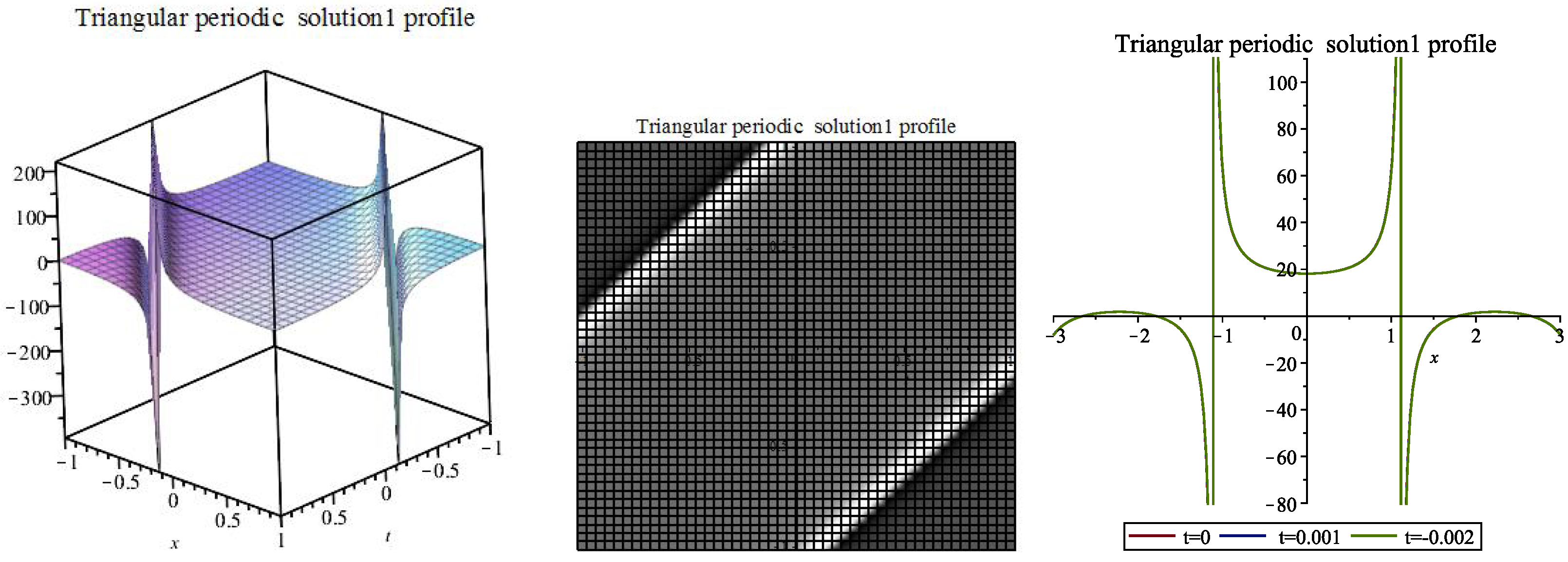
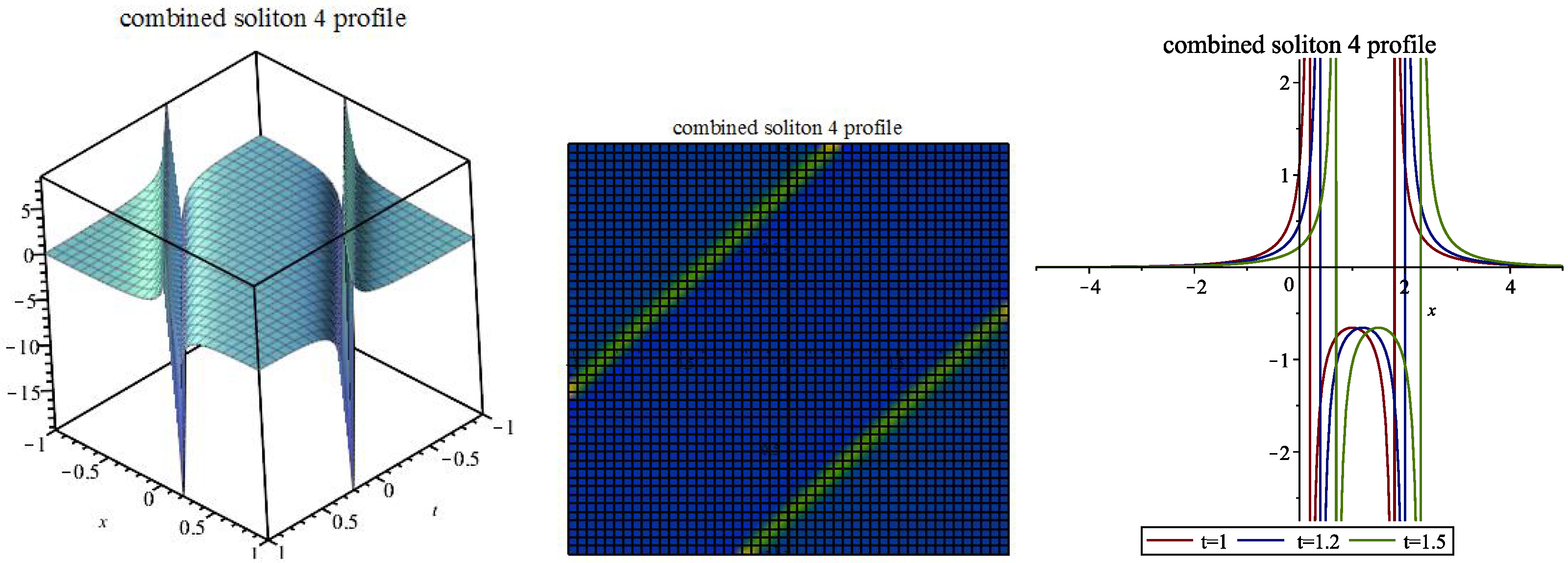
5. Analysis of Solutions and Graphical Depictions

The exploration of the various dynamical behaviour of the secured solutions for the (1+1)D-gvcKdVDampe (3) is performed via its physical interpretation. This is exhibited through numerical simulations which is being effected by making suitable choice of the involved arbitrary functions or/and constants appearing in the obtained results. We engaged a fruitful process involved in F-expansion technique to secure diverse multi-solitons, bright soliton solutions, dark soliton solution, singular soliton, topological kink as well as periodic soliton solutions. Numerical simulation of these solutions occasioned the depiction of triangular periodic solutions (60)–(62) in Figure 1, Figure 2 and Figure 3, respectively. We portrayed the first solution using 3D, density and 2D plots in the first Figure with dissimilar parameter values $a_2=-2$, $a_4=3$, $n=1$, $\alpha =0.2$, $k_0=1$, $\nu =1$ with $-1\le t,x\le 1$ where the representation reveals that the solution is singular at points $x=-1$ and $x=1$. In the case of (61) we reveal its dynamics in Figure 2 through 3D, 2D as well as density plots using constant values $a_2=-2$, $a_4=1$, $n=1$, $\alpha =0.2$, $k_0=1$, $\nu =1$ and variables $-2\le t,x\le 2$. The pictorial portrayal in this case shows that the solution has singularities at $x=-4$, $x=-2$, $x=0$ and $x=3$. Further, two-dimensional, three-dimensional and density plots in Figure 3 exhibits the motion of singular periodic solution (62) with unalike values $a_2=2$, $a_4=1$, $n=1$, $\alpha =1$, $k_0=1$, $\nu =1$ with variables $-5\le t,x\le 5$. This instance shows points of singularity in the domain of $-4\le x\le 4$. The bell-shaped solitary wave structures in Figure 4 and Figure 5 accordingly depict bright soliton solution (63) with parametric values $a_2=1$, $a_4=-1$, $n=1$, $\alpha =2$, $k_0=1$, $\nu =1$ and $-2\le t,x\le 2$ with $a_2=1$, $a_4=-1$, $n=1$, $\alpha =2$, $k_0=1$, $\nu =1$ and variables $-6\le t,x\le 6$. Further, Figure 4 is notable in the sense that the bright soliton wave shows a compact-type wave structure which is pertinent. Moreover, cosecant hyperbolic function solution (64) is portrayed in Figure 6 via 3D, 2D together with density plots with constant values $a_2=2$, $a_4=-1$, $n=1$, $\alpha =0.2$, $k_0=1$, $\nu =1$ together with variables $-1\le t,x\le 1$. The solution exhibits singularities in the region $0\le x\le 0.5$. The topological kink soliton solution (65) is depicted with graphs in two dimensions, three dimensions as well as density plots in Figure 7 with unalike constant values $a_2=-2$, $a_4=2$, $n=1$, $\alpha =0.2$, $k_0=1$, $\nu =1$ alongside variables $-3\le t,x\le 3$.

The combined soliton (67) was graphically represented in Figure 8 and Figure 9 giving dark soliton wave structures. The parametric values used in plotting the Figures are, respectively, $a_2=1$, $a_3=1$, $a_4=-1$, $n=1$, $c_1=5$, $k_0=1$, $\nu =1$ and $-3\le t,x\le 3$ with $a_2=1$, $a_3=7$, $a_4=-1$, $n=1$, $c_1=5$, $k_0=4$, $\nu =1$ alongside $-3\le t,x\le 3$. We depict merged soliton solution (68) with anti-bell shaped wave in Figure 10 via 3D, density and 2D plots using constant values $a_2=6$, $a_3=8$, $a_4=1$, $n=1$, $\beta =-1$, $k_0=1$, $\nu =1$ with variables t and x in the interval $-4\le t,x\le 4$. The bell-shaped wave structure in Figure 11 reveals the dynamical character of combined soliton solution of (21) in (69) where we implore the values $a_2=6$, $a_3=8$, $a_4=1$, $n=1$, $\beta =-1$, $k_0=1$, $\nu =1$ and $-4\le t,x\le 4$. Furthermore, 3D plot, 2D plot and density plot in Figure 12 shows the influence of (70) by engaging constant values $a_2=1$, $a_3=3$, $a_4=1$, $n=1$, $c_1=1$, $k_0=1$, $\nu =1$ alongside variables $-1\le t,x\le 1$. The dynamical wave behaviour of soliton solution (71) is exhibited.

In Figure 13 with parameters $a_2=1$, $a_3=4$, $a_4=1$, $n=1$, $\beta =-1$, $k_0=1$, $\nu =1$ where t and x exist in interval $-2\le t,x\le 2$. We notice that (70) and (71) both reveal singularities in the domain $0\le x\le 2$. Now, we depict the Jacobi elliptic solutions obtained for Equation (21) using Figures in two and three dimensions alongside density plots. Elliptic solutions (74) and (75) are depicted in Figure 14 and Figure 15 accordingly using parametric values $n=1$, $\beta =-1$, $k_0=0.6$, $\nu =7$ with $-3\le t,x\le 3$ as well as $n=2$, $\beta =-1$, $k_0=0.5$, $\nu =4$ with $-2.5\le t,x\le 2.5$. We also reveal the motions behaviour of (82) with Figure 16 and Figure 17 where we invoke, respectively, $n=2$, $\beta =-1$, $k_0=1$, $\nu =1$ whereas $-3\le t,x\le 3$ and $n=1$, $\beta =-1$, $k_0=2$, $\nu =3$ along with t and x in the same interval. It is observed that when $n=1$, we have a sinusoidal wave structure with the wave travelling with uniform frequency and amplitude whereas at $n=2$ the solution gives a combined dark and bright soliton wave structure behaving in similar manner. In addition to that, Figure 15 and Figure 17 reveal W-shaped soliton wave structures through the 2D plots. Moreover, periodic soliton solution (84) reveals a constant amplitude and frequency in its wave propagation as depicted in Figure 18 using parametric values $n=1$, $\beta =-1$, $k_0=1.1$, $\nu =1.1$ and variables $-8\le t,x\le 8$. Finally, we exhibit the character of elliptic solution (89) in Figure 19 with constant values $n=1$, $\beta =-1$, $k_0=1$, $\nu =3$ where we have $-7\le t,x\le 7$. The three-dimensional plot shows a multi-soliton wave structure of the solution.

Observations

We specifically noticed that the wave profiles in Figure 4 and Figure 7 give a pulse-compacton and a kink-compacton wave structures, respectively, while profiles in Figure 8 and Figure 9 exhibit partial pulse-compactons. Compacton is defined as a robust and strictly localized nonlinear wave which unlike soliton (a solitary wave that asymptotically retains its shape together with velocity upon collision with another solitary wave) is characterized by the absence of infinitesimal wings extending to infinity [50]. It also has a profile or spatial width that is independent of its velocity. A crucial building block for the existence of compactons is nonlinear dispersion. These can as well be generated in a continuum system dependent on the interplay between dispersive and nonlinear phenomena. On the other hand, wave profiles in Figure 5, Figure 10 and Figure 11 reveal pulse-soliton wave structures.

Solitons and Classical Solutions in Quantum Field Theory

Soliton theory is an essential branch of applied mathematics as well as mathematical physics. It is a highly active and productive field of research and also has important applications in diverse fields of science, such as fluid mechanics, nonlinear optics, classical and quantum fields theories.

Solitons are solutions of classical field equations which possess particle-like attributes. In addition to that, they are localized in space and have finite energy. They are also stable against decay into radiation. They further give rise to new particle states in the underlying quantum field theory, after quantization, which is not seen in perturbation theory. The stability property possessed by solitons usually has a topological explanation.

Given a classical field theory, in a bid to “quantize” it, the vacuum of the theory will be found and then perturbation theory around this vacuum are done. Suppose there are multiple vacua, then an arbitrary vacuum is picked and expansion is done around it. However, these fields theories possessing multiple vacua often contain soliton solutions. In addition, these solutions are localized smooth solutions of classical field equations which connect multiple vacuums. This process in the case of kink soliton solution is known as spontaneous symmetry breaking. Of course, by virtue of symmetry, one obtains the same quantum theory regardless of which vacuum one expands around where the kink stability comes from the topology. In order to quantize these solitons solutions, one fixes such a soliton and thereafter utilizes it as the “background”. In consequence, one then invokes perturbation theory around these solutions, although this is quite tricky to do. Hence, in a lot of courses, physicists just examine the classical part of the theory. It is to recall that when quantizing field theories in perturbation theory, one obtains particles in the sense of quantum theory, despite the classical theory being completely about fields. It turns out that solitons also act just like particles which are a new type of particles. These are referred to as non-perturbative phenomenon. If one actually wants to do the quantum field theory properly, then the inclusion of these solitons in the quantum field theory is needed.

Therefore, in diverse cases, one discovers that classical field equations possess solutions that suggest a particle interpretation. They are localized with the concentration of their energy density within a fairly well-defined region of space. Outside this region, the involved fields quickly approach their vacuum values. These solutions are found out to be stable and sustain their structure as time goes on. Moreover, they can be enhanced to yield linearly moving solutions. These are seen to carry linear momentum and also display the proper relationship between energy, mass as well as momentum. The existent of soliton called objects depends essentially on the nonlinear manner of the field equations. This in turn is revealed in their non-analytic character as the coupling constants of the theory approach zero. Precisely, the soliton mass typically diverges in this limit, thus acting as an inverse of a coupling constant. Second class solutions called the nontopological solitons are in the same vein stabilized by a conserved charge carried by the soliton. Nonetheless, in this regard, the charge is of the same kind as that carried by the elementary particles of the theory. In order to make stable soliton exist, one must ensure that mass to charge ratio must be small enough to restrain decay by emission of these elementary charged particles. Thus, for the afore-discussed solutions, the quantum interpretation is a straightforward extension of the classical meaning [51]. Another important area of study is the application of solitons to describe nonperturbative phenomena in quantum field theory.

In the case of the effect of multi-solitons in quantum field theory, It has been revealed that one would not ordinarily expect to get static solutions that delineate spatially separated solitons, due to the fact that, at any finite distance there would be nonzero inter-soliton forces. A static multisoliton solution would need a remarkable cancellation existent between the attractive as well as the repulsive forces that are prevalent. Nevertheless, the exact proportionality between energy alongside the topological charge of Bogomolny-type first-order differential Equation (BPS) solutions suggests that just such a cancellation might take place. In fact, we have seen that in the BPS monopole the Higgs field has a certain tail that corresponds to a long-range attractive force which possesses the potential to exactly nullify the magnetic repulsion [52].

We are aware that the solutions constructed comprises, elliptic wave solutions (whose special limits yield hyperbolic and elementary trigonometric functions), periodic, hyperbolic as well as trigonometric functions with various applications in theoretical physics. The benefit of such functions is that the wave’s physical behaviour can be effortlessly commented on, irrespective of the graph’s range which the resulting solution function owns. Mathematical functions such as trigonometric, as well as hyperbolic, arise in physical sciences. Example of this is the case of hyperbolic cosine functions that possesses the shape of a catenary which by extension is applied in delineating satellite rings’ formed around planets. Furthermore, they are also applicable in the theory of special relativity. Besides, in quantum physics, tan-hyperbolic functions emerge in calculating the rapidity of special relativity and magnetic moment. In the laminar jet’s profile, secant hyperbolic functions appear. Moreover, in Langevin function for polarization of magnets, cotangent hyperbolic functions come to fore [53].

Furthermore, a classical solution is a function that solves a given partial differential equation in the usual sense. For instance, for unidirectional wave equation given as $u_t+u_x=0$, any function of the structure $u(t,x)=f(t-x)$ where f is twice differentiable is a classical solution of the wave equation. Consequently, classical solutions such as are secured in this study play an important role in quantum field theory, high energy physics and cosmology. Real-time soliton solutions give rise to the emergence of particles which include magnetic monopoles as well as extended structures, such as domain walls and cosmic strings. These in turn have implications for early universe cosmology. Besides, imaginary-time Euclidean instantons are responsible for important nonperturbative effects whereas Euclidean bounce solutions govern transitions between metastable states.

6. Synopsis of Conservation Laws for (3)

In this section, we compute the conservation laws of Equation (3) for various cases including when function $H(t)\ne 0$ and when $H(t)=0$, using both the direct approach and Noether’s theorem where applicable.

6.1. Conserved Currents of Equation (3) When $n=m$

We seek the multipliers of (3) here with a view to using them to construct the conserved currents of the equation when $n=m$.

6.1.1. Application of Direct Technique

We construct the conserved currents of (16) first for two cases of $Q(t)$ and $S(t)$ using the direct approach [54].

Case 1A$Q(t)=A{(\beta +t)}^{-\frac{1}{3}(3\alpha n+3\beta n+n+2)}{e}^{nt},S(t)=B{(\beta +t)}^{\frac{2}{3}(-3\alpha n-3\beta n-n-1)}{e}^{2nt}$.

In this case, we insert the expressions for $Q(t)$ and $S(t)$ in (16) and then we have:

$$\begin{array}{cc}\hfill & u_t+A{(\beta +t)}^{-\frac{1}{3}(3\alpha n+3\beta n+n+2)}{e}^{nt}{u}^n{u}_x+B{(\beta +t)}^{\frac{2}{3}(-3\alpha n-3\beta n-n-1)}{e}^{2nt}{u}^{2n}{u}_x\hfill \\ \hfill & +u+u_{xxx}=0.\hfill \end{array}$$

(95)

We commence the application of the technique by using the zeroth order multiplier $\mathsf{\Lambda }=\mathsf{\Lambda }(t,x,u)$ in the required equation expressed in this regard simply as:

$$\begin{array}{cc}\hfill & \left\{\frac{\partial }{\partial u}-D_t\frac{\partial }{\partial u_t}-D_x\frac{\partial }{\partial u_x}-D_t\frac{\partial }{\partial u_t}-D_x^3\frac{\partial }{\partial u_{xxx}}\right\}[\mathsf{\Lambda }(u_t+A{(\beta +t)}^{-\frac{1}{3}(3\alpha n+3\beta n+n+2)}\hfill \\ \hfill & \times e^{nt}{u}^n{u}_x+B{(\beta +t)}^{\frac{2}{3}(-3\alpha n-3\beta n-n-1)}{e}^{2nt}{u}^{2n}{u}_x+u+u_{xxx})]=0.\hfill \end{array}$$

(96)

Further expansion of (96), splitting the outcome on diverse included derivatives of u and further simplifying the obtained equations yields the system of equations

$$\begin{array}{cc}\hfill & {\mathsf{\Lambda }}_{ux}=0,{\mathsf{\Lambda }}_{uu}=0,{(t+\beta )}^{2\alpha n+2\beta n+2/3}u{\mathsf{\Lambda }}_u+{(t+\beta )}^{2\alpha n+2\beta n+2/3}\mathsf{\Lambda }\hfill \\ \hfill & -{(t+\beta )}^{2\alpha n+2\beta n+2/3}{\mathsf{\Lambda }}_t-A{(t+\beta )}^{\alpha n+2\beta n-n/3+2/3}{u}^n{e}^{nt}{\mathsf{\Lambda }}_x\hfill \\ \hfill & -B{(t+\beta )}^{-2n/3}{u}^{2n}{e}^{2nt}{\mathsf{\Lambda }}_x-{(t+\beta )}^{2\alpha n+2\beta n+2/3}{\mathsf{\Lambda }}_{xxx}=0.\hfill \end{array}$$

(97)

Solving the three system of equations gives the value of $\mathsf{\Lambda }(t,x,u)$ as:

$$\mathsf{\Lambda }(t,x,u)=C_1{e}^{2t}u+C_2{e}^t,$$

(98)

where $C_1$ and $C_2$ are constants. Next, to gain the conserved currents of Equation (95), we have to engage the divergence relation which we present in this regard as:

$$\begin{array}{cc}\hfill D_{t}T+D_{x}X=& [u_t+A{(\beta +t)}^{-\frac{1}{3}(3\alpha n+3\beta n+n+2)}{e}^{nt}{u}^n{u}_x+B{(\beta +t)}^{\frac{2}{3}(-3\alpha n-3\beta n-n-1)}\hfill \\ \hfill & \times e^{2nt}{u}^{2n}{u}_x+u+u_{xxx}]\mathsf{\Lambda }(t,x,u),\hfill \end{array}$$

(99)

where the conserved currents $(T_i,X_i),i=1,2$ are computed. Thus, from (99), a quite lengthy calculations would give the general case for the conserved currents as:

$$\begin{array}{cc}\hfill T=& \frac{1}{2}u{e}^t\left(C_1{e}^{t}u+2C_2\right),\hfill \\ \hfill X=& \frac{1}{2(n+1)(n+2)(2n+1)}\{4e^{2t}{n}^{3}u{u}_{xx}{C}_1-2e^{2t}{n}^3{u}_x^2{C}_1+14e^{2t}{n}^{2}u{u}_{xx}{C}_1\hfill \\ \hfill & +4A{e}^{t(n+2)}{(\beta +t)}^{-\alpha n-\beta n-\frac{1}{3}n-\frac{2}{3}}{u}^{n+2}{n}^2{C}_1+2B{e}^{2t(n+1)}{(\beta +t)}^{-\frac{2}{3}n-2\alpha n-2\beta n-\frac{2}{3}}\hfill \\ \hfill & \times u^{2n+2}{n}^2{C}_1-7e^{2t}{n}^2{u}_x^2{C}_1+14e^{2t}nu{u}_{xx}{C}_1+4e^t{n}^3{u}_{xx}{C}_2+6A{e}^{t(n+2)}\hfill \\ \hfill & \times {(\beta +t)}^{-\alpha n-\beta n-\frac{1}{3}n-\frac{2}{3}}{u}^{n+2}n{C}_1+5B{e}^{2t(n+1)}{(\beta +t)}^{-\frac{2}{3}n-2\alpha n-2\beta n-\frac{2}{3}}{u}^{2n+2}n{C}_1\hfill \\ \hfill & -7e^{2t}n{u}_x^2{C}_1+4C_1{e}^{2t}u{u}_{xx}+14e^t{n}^2{u}_{xx}{C}_2+2A{e}^{t(n+2)}{(\beta +t)}^{-\alpha n-\beta n-\frac{1}{3}n-\frac{2}{3}}\hfill \\ \hfill & \times C_1{u}^{n+2}+4A{e}^{t(n+1)}{(\beta +t)}^{-\alpha n-\beta n-\frac{1}{3}n-\frac{2}{3}}{u}^{n+1}{n}^2{C}_2+2B{e}^{2t(n+1)}\hfill \\ \hfill & \times {(\beta +t)}^{-\frac{2}{3}n-2\alpha n-2\beta n-\frac{2}{3}}{C}_1{u}^{2n+2}+2B{e}^{t(2n+1)}{(\beta +t)}^{-\frac{2}{3}n-2\alpha n-2\beta n-\frac{2}{3}}{u}^{2n+1}\hfill \\ \hfill & \times n^2{C}_2-2C_1{e}^{2t}{u}_x^2+14e^{t}n{u}_{xx}{C}_2+10A{e}^{t(n+1)}{(\beta +t)}^{-\alpha n-\beta n-\frac{1}{3}n-\frac{2}{3}}{u}^{n+1}n{C}_2\hfill \\ \hfill & \times +6B{e}^{t(2n+1)}{(\beta +t)}^{-\frac{2}{3}n-2\alpha n-2\beta n-\frac{2}{3}}{u}^{2n+1}n{C}_2+4e^t{u}_{xx}{C}_2+4A{e}^{t(n+1)}\hfill \\ \hfill & \times {(\beta +t)}^{-\alpha n-\beta n-\frac{1}{3}n-\frac{2}{3}}{C}_2{u}^{n+1}+4B{e}^{t(2n+1)}{(\beta +t)}^{-\frac{2}{3}n-2\alpha n-2\beta n-\frac{2}{3}}{C}_2{u}^{2n+1}\},\hfill \end{array}$$

(100)

where $n\ne -2,-1,-1/2$. Thus, we gain the two conserved currents of (16) here as:

$$\begin{array}{cc}\hfill T_1=& \frac{1}{2}{u}^2{e}^{2t},\hfill \\ \hfill X_1=& \frac{1}{2(n+1)(n+2)}\{2nA{e}^{t(n+2)}{(\beta +t)}^{-\alpha n-\beta n-\frac{1}{3}n-\frac{2}{3}}{u}^{n+2}\hfill \\ \hfill & +n{u}^{2n+2}B{e}^{2t(n+1)}{(\beta +t)}^{-2\alpha n-2\beta n-\frac{2}{3}n-\frac{2}{3}}+2e^{2t}{n}^{2}u{u}_{xx}-e^{2t}{n}^2{u}_x^2\hfill \\ \hfill & +2A{e}^{t(n+2)}{(\beta +t)}^{-\alpha n-\beta n}{(\beta +t)}^{-\frac{1}{3}n-\frac{2}{3}}{u}^{n+2}+6e^{2t}nu{u}_{xx}\hfill \\ \hfill & +2B{e}^{2t(n+1)}{u}^{2n+2}{(\beta +t)}^{-2\alpha n-2\beta n-\frac{2}{3}n-\frac{2}{3}}-3e^{2t}n{u}_x^2+4e^{2t}u{u}_{xx}-2e^{2t}{u}_x^2\};\hfill \\ \\ \hfill T_2=& u{e}^t,\hfill \\ \hfill X_2=& \frac{1}{(2n+1)(n+1)}\{2nA{e}^{t(n+1)}{(\beta +t)}^{-\alpha n-\beta n-\frac{1}{3}n-\frac{2}{3}}{u}^{n+1}\hfill \\ \hfill & +n{u}^{2n+1}B{e}^{t(2n+1)}{(\beta +t)}^{-2\alpha n-2\beta n-\frac{2}{3}n-\frac{2}{3}}+A{e}^{t(n+1)}{(\beta +t)}^{-\alpha n-\beta n-\frac{1}{3}n-\frac{2}{3}}{u}^{n+1}\hfill \\ \hfill & +B{e}^{t(2n+1)}{u}^{2n+1}{(\beta +t)}^{-2\alpha n-2\beta n-\frac{2}{3}n-\frac{2}{3}}+2e^t{n}^2{u}_{xx}+3e^{t}n{u}_{xx}+e^t{u}_{xx}\}.\hfill \end{array}$$

Case 1B$Q(t)=A{e}^{-\lambda nt},S(t)=B{e}^{-2\lambda nt}$,

We insert the given functions in Equation (16) and obtain the differential equation

$$\begin{array}{c}\hfill u_t+A{e}^{-\lambda nt}{u}^n{u}_x+B{e}^{-2\lambda nt}{u}^{2n}{u}_x+u+u_{xxx}=0.\end{array}$$

(101)

On engaging the steps adopted in (96)–(97), we achieve the multiplier

$$\mathsf{\Lambda }(t,x,u)=C_1{e}^{2t}u+C_2{e}^t.$$

(102)

In consequence, we gain the conserved currents of Equation (3) in this regard as:

$$\begin{array}{cc}\hfill T_1=& \frac{1}{2}{e}^{2t}{u}^2,\hfill \\ \hfill X_1=& \frac{1}{2(n+1)(n+2)}\{2e^{2t}{n}^{2}u{u}_{xx}-e^{2t}{n}^2{u}_x^2+2An{u}^{n+2}{e}^{-t(\lambda n-2)}\hfill \\ \hfill & +Bn{u}^{2n+2}{e}^{-2t(\lambda n-1)}+6e^{2t}nu{u}_{xx}-3e^{2t}n{u}_x^2+2A{e}^{-t(\lambda n-2)}{u}^{n+2}\hfill \\ \hfill & +2B{e}^{-2t(\lambda n-1)}{u}^{2n+2}+4e^{2t}u{u}_{xx}-2e^{2t}{u}_x^2\};\hfill \\ \\ \hfill T_2=& u{e}^t,\hfill \\ \hfill X_2=& \frac{1}{(2n+1)(n+2)}\{2An{u}^{n+1}{e}^{-t(\lambda n-1)}+Bn{u}^{2n+1}{e}^{-t(2\lambda n-1)}+2e^t{n}^2{u}_{xx}\hfill \\ \hfill & +A{e}^{-t(\lambda n-1)}{u}^{n+1}+B{u}^{2n+1}{e}^{-t(2\lambda n-1)}+3e^{t}n{u}_{xx}+e^t{u}_{xx}\}.\hfill \end{array}$$

6.1.2. Conserved Currents of (21)

We seek the multipliers of (21) here and then use them to construct the conserved currents of the equation when $n=m$.

Case 2A$Q(t)=A{(\varphi +t)}^{-\frac{1}{3}(3\theta n+n+2)},S(t)=B{(\varphi +t)}^{\frac{2}{3}(-3\theta n-n-1)}$.

In this case, we insert the expressions for $Q(t)$ and $S(t)$ in (21) and then we have:

$$\begin{array}{c}\hfill u_t+A{t}^{-\frac{1}{3}(3\theta n+n+2)}{u}^n{u}_x+B{t}^{\frac{2}{3}(-3\theta n-n-1)}{u}^{2n}{u}_x+u_{xxx}=0,\mathrm{with}\varphi =0.\end{array}$$

(103)

On utilizing the relation expressed in (96), we secure the determining equations

$$\begin{array}{cc}\hfill & {\mathsf{\Lambda }}_{ux}=0,{\mathsf{\Lambda }}_{uu}=0,t^{2\theta n+2/3}{\mathsf{\Lambda }}_t+A{t}^{\theta n-n/3}{u}^n{e}^{nt}{\mathsf{\Lambda }}_x+B{t}^{-2n/3}{u}^{2n}{e}^{2nt}{\mathsf{\Lambda }}_x\hfill \\ \hfill & +t^{2\theta n+2/3}{\mathsf{\Lambda }}_{xxx}=0.\hfill \end{array}$$

(104)

Solving the system of equation presented in (104) gives the value of $\mathsf{\Lambda }(t,x,u)$ as:

$$\mathsf{\Lambda }(t,x,u)=C_{1}u+C_2,$$

(105)

with constants $C_1$ and $C_2$. On utilizing the divergence criteria earlier given in conjunction with homotopy formula gives us the conserved currents of (17) as

$$\begin{array}{cc}\hfill T_1=& \frac{1}{2}{u}^2,\hfill \\ \hfill X_1=& \frac{1}{2(2n+1)(n+1)(n+2)}\{4u{u}_{xx}-2n^3{u}_x^2-7n^2{u}_x^2-7n{u}_x^2\hfill \\ \hfill & +2A{t}^{-\theta n-\frac{1}{3}n-\frac{2}{3}}{e}^{nt}{u}^{n+2}+2B{t}^{-2\theta n-\frac{2}{3}n-\frac{2}{3}}{e}^{2nt}{u}^{2n+2}-2u_x^2\hfill \\ \hfill & +4A{t}^{-\theta n-\frac{1}{3}n-\frac{2}{3}}{e}^{nt}{n}^2{u}^{n+2}+6A{t}^{-\theta n-\frac{1}{3}n-\frac{2}{3}}{e}^{nt}n{u}^{n+2}+2B{t}^{-2\theta n-\frac{2}{3}n-\frac{2}{3}}{e}^{2nt}{n}^2{u}^{2n+2}\hfill \\ \hfill & +5B{t}^{-2\theta n-\frac{2}{3}n-\frac{2}{3}}{e}^{2nt}n{u}^{2n+2}+4n^{3}u{u}_{xx}+14n^{2}u{u}_{xx}+14nu{u}_{xx}\};\hfill \\ \\ \hfill T_2=& u,\hfill \\ \hfill X_2=& \frac{1}{(2n+1)(n+1)(n+2)}\{2n^3{u}_{xx}+7n^3{u}_{xx}+7n{u}_{xx}+2A{t}^{-\theta n-\frac{1}{3}n-\frac{2}{3}}{e}^{nt}{u}^{n+1}\hfill \\ \hfill & +2B{t}^{-2\theta n-\frac{2}{3}n-\frac{2}{3}}{e}^{2nt}{u}^{2n+1}+2A{t}^{-\theta n-\frac{1}{3}n-\frac{2}{3}}{e}^{nt}{n}^2{u}^{n+1}+5A{t}^{-\theta n-\frac{1}{3}n-\frac{2}{3}}{e}^{nt}n{u}^{n+1}\hfill \\ \hfill & +B{t}^{-2\theta n-\frac{2}{3}n-\frac{2}{3}}{e}^{2nt}{n}^2{u}^{2n+1}+3B{t}^{-2\theta n-\frac{2}{3}n-\frac{2}{3}}{e}^{2nt}n{u}^{2n+1}+2u_{xx}\}.\hfill \end{array}$$

Remark 3.

We note here that one of the multipliers from (105) is ${\mathsf{\Lambda }}_2=1$ and so signals the fact that Equation (103) is itself a conserved current and by extension represents conservation of energy.

Case 2B$Q(t)=A{e}^{-\varphi nt},S(t)=B{e}^{-2\varphi nt}$.

Thus, reckoning the exponential functions in (21), we have the equation

$$\begin{array}{c}\hfill u_t+A{e}^{-\varphi nt}{u}^n{u}_x+B{e}^{-2\varphi nt}{u}^{2n}{u}_x+u_{xxx}=0.\end{array}$$

(106)

Now, following the procedure taken in Equations (103)–(105), we gain two multipliers ${\mathsf{\Lambda }}_1=u$ and ${\mathsf{\Lambda }}_2=1$, thus, we consequently gain vectors presented as:

$$\begin{array}{cc}\hfill T_1=& \frac{1}{2}{u}^2,\hfill \\ \hfill X_1=& \frac{1}{2(2n+1)(n+1)(n+2)}\{2B{n}^2{u}^{2n+2}+5Bn{u}^{2n+2}+2A{u}^{n+2}{e}^{\varphi nt}-2n^3{u}_x^2{e}^{2\varphi nt}\hfill \\ \hfill & -7n^2{u}_x^2{e}^{2\varphi nt}-7n{u}_x^2{e}^{2\varphi nt}+4u{u}_{xx}{e}^{2\varphi nt}+2B{u}^{2n+2}-2e^{2\varphi nt}{u}_x^2+14e^{2\varphi nt}nu{u}_{xx}\hfill \\ \hfill & +4e^{2\varphi nt}{n}^{3}u{u}_{xx}+14n^2{e}^{2\varphi nt}u{u}_{xx}+6A{e}^{\varphi nt}n{u}^{n+2}+4A{e}^{\varphi nt}{n}^2{u}^{n+2}\};\hfill \\ \\ \hfill T_2=& u,\hfill \\ \hfill X_2=& \frac{1}{(2n+1)(n+1)(n+2)}\{2e^{2\varphi nt}{n}^3{u}_{xx}+2A{e}^{\varphi nt}{n}^2{u}^{n+1}+7n^2{e}^{2\varphi nt}{u}_{xx}+2u_{xx}\hfill \\ \hfill & +5A{e}^{\varphi nt}n{u}^{n+1}+B{n}^2{u}^{2n+1}+7e^{2\varphi nt}n{u}_{xx}+2A{e}^{\varphi nt}{u}^{n+1}+3Bn{u}^{2n+1}\hfill \\ \hfill & +2B{e}^{-2\varphi nt}{u}^{2n+1}\}.\hfill \end{array}$$

Moreover, we state here that remark (3) also applies in the case of $(T_2,X_2)$.

6.2. Conserved Currents of Equation (3) When $n\ne m$

Conserved Currents of (3) via Homotopy Formula

This subsubsection seeks to derive the conserved currents of Equations (16) and (21) when $n\ne m$ via their various multipliers using the homotopy formula.

On adopting the procedure outlined in Section 6.1, we secure the zeroth-order multiplier for Equations (16) and (21) for $Q(t)=S(t)=1$, respectively, as:

$$\begin{array}{cc}\hfill {\mathsf{\Lambda }}_1(t,x,u)=& A_{1}u+A_2,\hfill \end{array}$$

(107)

$$\begin{array}{cc}\hfill {\mathsf{\Lambda }}_2(t,x,u)=& A_1{e}^{2t}u+A_2{e}^t,\hfill \end{array}$$

(108)

where $A_1$ and $A_2$ are constants. Therefore, we have multipliers ${\mathsf{\Lambda }}_1$ and ${\mathsf{\Lambda }}_2$ constituting the conservation laws. Thus, we have the proposition and succeeding theorems to this effect.

Proposition 1.

All low-order multipliers (107) admitted by the underlying Equation (1+1)D-gvcKdVDampe (17) with functions $Q(t)=S(t)=H(t)=G(t)\ne 0$ give rise to conservation laws. The underlying multipliers are given by:

(i) multipliers of (16) where arbitrary $Q(t)=1=S(t)$ and $n\ne m$

$$\begin{array}{cc}\hfill & {\mathsf{\Lambda }}_{1a}=u,\hfill \end{array}$$

(109)

$$\begin{array}{cc}\hfill & {\mathsf{\Lambda }}_{1b}=1.\hfill \end{array}$$

(110)

(ii) multipliers of (21) with arbitrary $Q(t)=S(t)=1$ and $n\ne m$:

$$\begin{array}{cc}\hfill & {\mathsf{\Lambda }}_{2a}=e^{2t}u,\hfill \end{array}$$

(111)

$$\begin{array}{cc}\hfill & {\mathsf{\Lambda }}_{2b}=e^t.\hfill \end{array}$$

(112)

Theorem 1.

The conserved current admitted by Equation (1+1)D-gvcKdVDampe (3) for low-order multiplier ${\mathsf{\Lambda }}_1$ with integer exponent $n\ne m$ are presented as:

Case 1a: $n\ne -1,-2$, $m\ne -1/2,-1$

$$\begin{array}{cc}\hfill T_{1a}^t=& \frac{1}{2}{u}^2,\hfill \\ \hfill X_{1a}^x=& \frac{1}{2(2m+1)(m+1)(n+1)(n+2)}\{2u^{2m+2}-3m{n}^2{u}_x^2+8m^{2}u{u}_{xx}+2n^{2}u{u}_{xx}\hfill \\ \hfill & +12mu{u}_{xx}+6nu{u}_{xx}-2m^2{n}^2{u}_x^2-6m^{2}n{u}_x^2+6m{n}^{2}u{u}_{xx}-9mn{u}_x^2-4m^2{u}_x^2\hfill \\ \hfill & -n^2{u}_x^2-6m{u}_x^2-3n{u}_x^2+18nmu{u}_{xx}+4m^2{n}^{2}u{u}_{xx}+12m^{2}nu{u}_{xx}+2u^{n+2}\hfill \\ \hfill & -2u_x^2+3n{u}^{2m+2}+4m{u}^{2m+2}+4u{u}_{xx}+2n{u}^{n+2}+n^2{u}^{2m+2}+6m{u}^{n+2}\hfill \\ \hfill & +4m^2{u}^{n+2}+2m{n}^2{u}^{2m+2}+6mn{u}^{2m+2}+4m^{2}n{u}^{n+2}+6mn{u}^{n+2}\};\hfill \end{array}$$

Case 1b: $n\ne -1,-2$, $m\ne -1/2,-1$

$$\begin{array}{cc}\hfill T_{1b}^t=& u,\hfill \\ \hfill X_{1b}^x=& \frac{1}{(2m+1)(m+1)(n+1)(n+2)}\{2u^{2m+1}+2u^{n+1}+2u_{xx}+n{u}^{n+1}+6m{u}^{n+1}\hfill \\ \hfill & +4m^2{u}_{xx}+n^2{u}_{xx}+9mn{u}_{xx}+m{n}^2{u}^{2m+1}+3mn{u}^{2m+1}+2m^{2}n{u}^{n+1}\hfill \\ \hfill & +3mn{u}^{n+1}+6m{u}_{xx}+3n{u}_{xx}+2m{u}^{2m+1}+3n{u}^{2m+1}+n^2{u}^{2m+1}+4m^2{u}^{n+1}\hfill \\ \hfill & +2m^2{n}^2{u}_{xx}+6m^{2}n{u}_{xx}+3m{n}^2{u}_{xx}\}.\hfill \end{array}$$

Moreover, the corresponding conservation laws of (21) obtained via ${\mathsf{\Lambda }}_2$ are:

Case 2a: $n\ne -1,-2$, $m\ne -1/2,-1$

$$\begin{array}{cc}\hfill T_{2a}^t=& \frac{1}{2}{e}^{2t}{u}^2,\hfill \\ \hfill X_{2a}^x=& \frac{e^{2t}}{2(2m+1)(m+1)(n+1)(n+2)}\{8m^{2}u{u}_{xx}-2m^2{n}^2{u}_x^2-6m^{2}n{u}_x^2\hfill \\ \hfill & -3m{n}^2{u}_x^2+2n{u}^{n+2}-9mn{u}_x^2+2n^{2}u{u}_{xx}+12mu{u}_{xx}+6nu{u}_{xx}\hfill \\ \hfill & +4m^{2}n{u}^{n+2}+2m{n}^2{u}^{2m+2}+6mn{u}^{n+2}+6mn{u}^{2m+2}+2u^{2m+2}\hfill \\ \hfill & +4u{u}_{xx}+2u^{n+2}-6m{u}_x^2-3n{u}_x^2+4m^2{u}^{n+2}+n^2{u}^{2m+2}+3n{u}^{2m+2}\hfill \\ \hfill & -4m^2{u}_x^2-n^2{u}_x^2+4m{u}^{2m+2}+6m{u}^{n+2}+12m^{2}nu{u}_{xx}+6m{n}^{2}u{u}_{xx}\hfill \\ \hfill & +18mnu{u}_{xx}-2u_x^2+4m^2{n}^{2}u{u}_{xx}\}\hfill \end{array}$$

Case 2b: $n\ne -1,-2$, $m\ne -1/2,-1$

$$\begin{array}{cc}\hfill T_{2b}^t=& e^{t}u,\hfill \\ \\ \hfill X_{2b}^x=& \frac{e^t}{(2m+1)(m+1)(n+1)(n+2)}\{2m^2{n}^2{u}_{xx}+2m^{2}n{u}^{n+1}+m{n}^2{u}^{2m+1}\hfill \\ \hfill & +6m^{2}n{u}_{xx}+3m{n}^2{u}_{xx}+4m^2{u}^{n+1}+3mn{u}^{n+1}+3mn{u}^{2m+1}+n^2{u}^{2m+1}\hfill \\ \hfill & +4m^2{u}_{xx}+9mn{u}_{xx}+n^2{u}_{xx}+6m{u}^{n+1}+n{u}^{n+1}+2m{u}^{2m+1}+3n{u}^{2m+1}\hfill \\ \hfill & +6m{u}_{xx}+3n{u}_{xx}+2u^{n+1}+2u^{2m+1}+2u_{xx}\}.\hfill \end{array}$$

It is noteworthy to state that remark (3) applies in the case of ${\mathsf{\Lambda }}_{1b}$ in (110).

Remark 4.

Having observed the conserved vectors achieved here, we notice interesting conservation laws with the existence of mass density as well as elastic energy density. Moreover, going by the multipliers obtained, momentum conservation law and conservation law of energy were also constructed.

6.3. Application of Noether’s Theorem

This subsection is dedicated to achieve the conserved currents of (3) for both cases of $n=m$ and $n\ne m$ when $H(t)=0$ by utilizing the novel Noether’s theorem [55].

6.3.1. Noether Conserved Currents of (3) When $n=m$, $H(t)=0$

We apply the classical Noether’s theorem [55,56] to gain various nonlocal and local conserved vectors of (17). Equation (3) with or without the variable-coefficient has no Lagrangian. However, taking $H(t)=0$, we recover a Lagrangian for the equation. We commence with the transformation $u=v_x$ with $G(t)=1$, which makes (21) become a variable-coefficient partial differential equation in $vs.$ as:

$$\begin{array}{c}\hfill v_{tx}+Q(t)v_x^n{v}_{xx}+S(t)v_x^{2n}{v}_{xx}+v_{xxxx}=0,\end{array}$$

(113)

with arbitrary $Q(t)$ and $S(t)$. We present a low-order differential Lagrangian of (113) in the Lemma given subsequently:

Lemma 1.

The variable-coefficient (1+1)D-gKdVDampe (21) forms the Euler–Lagrange equation with the functional

$$J(v)={\int }_0^{\infty }{\int }_0^{\infty }\mathcal{L}(t,x,v_t,v_x,v_{xx})dtdx$$

(114)

with conforming function of Lagrange $\mathcal{L}$ structured in a minimum differential order

$$\mathcal{L}=-\frac{1}{2}{v}_t{v}_x-\frac{Q(t)v_x^{n+2}}{(n+1)(n+2)}-\frac{S(t)v_x^{2n+2}}{(2n+1)(2n+2)}+\frac{1}{2}{v}_{xx}^2.$$

(115)

The proof of Lemma (1) is straightforward. We implore the invariant criteria

$${\mathrm{pr}}^{3}W(\mathcal{L})+\mathcal{L}{D}_t{\xi }^1+D_x{\xi }^2=D_t{B}^1+D_x{B}^2,$$

(116)

with $D_t,D_x$ as in (11) and the third prolongation of R attainable through relation

$${\mathrm{pr}}^{3}W=W+{\zeta }_t\frac{\partial }{\partial v_t}+{\zeta }_x\frac{\partial }{\partial v_x}+{\zeta }_{xx}\frac{\partial }{\partial v_{xx}}.$$

(117)

In addition, we define variational symmetries W as $W={\xi }^1\partial /\partial t+{\xi }^2\partial /\partial x+\eta \partial /\partial vs.$. Observe that functions ${\xi }^1$, ${\xi }^2$, $\eta$, $B^1$ as well as $B^2$ in (116) are dependent on $t,x$ and $vs.$. Performing Lie symmetry analysis procedure on invariance criteria (116) gives the system of linear partial differential equations (LPDEs) calculated as:

$$\begin{array}{cc}\hfill & {\xi }_x^1=0,{\xi }_u^1=0,{\xi }_t^2=0,{\eta }_x=0,B_x^2=0,{\xi }_u^2=0,{\eta }_t+2B_u^2=0,\hfill \\ \hfill & {\xi }_u^1+B_u^1=0,{\eta }_{uu}=0,2{\eta }_{ux}-{\xi }_{xx}^2=0,2{\eta }_u-3{\xi }_x^2-{\xi }_t^1-B_t^1=0,\hfill \\ \hfill & n{\xi }_u^1+{\xi }_u^1+B_u^1=0,2n{\xi }_u^1+{\xi }_u^1+B_u^1=0,B_t^1-2{\eta }_u=0,\hfill \\ \hfill & n{\eta }_u+2{\eta }_u-n{\xi }_x^2+{\xi }_t^1-{\xi }_x^2-B_t^1=0,\hfill \\ \hfill & 2n{\eta }_u+2{\eta }_u-2n{\xi }_x^2+{\xi }_t^1-{\xi }_x^2-B_t^1=0.\hfill \end{array}$$

Solving the system gives solutions for four cases of arbitrary $Q(t)$ and $S(t)$, viz:

Case a.$Q(t)=0$, $S(t)\ne 0$

In this case, the solution of the coefficient functions of the variational symmetry is

$$\begin{array}{cc}\hfill & {\xi }^1(t,x,v)=A_{1}t+A_2,{\xi }^2(t,x,v)=\frac{1}{3}{A}_{1}x+A_3,\eta (t,x,v)=\frac{n-1}{3n}{A}_{1}vs.+f_1(t),\hfill \\ \hfill & B^1(t,x,v)=\frac{2(n-1)}{3n}{A}_{1}t+f_2(x),B^2(t,x,v)=-\frac{1}{2}{f}_1^{\prime }(t)vs.+f_3(t),\hfill \end{array}$$

with arbitrary constants $A_1$, $A_2$, $A_3$ and functions $f_1(t)$ and $f_2(x)$ as well as $f_3(t)$, In consequence, we generate four Noether symmetries from the solution. They are:

$$\begin{array}{cc}\hfill W_1=& \frac{\partial }{\partial t},B^1=0,B^2=0,\hfill \\ \hfill W_2=& \frac{\partial }{\partial x},B^1=0,B^2=0,\hfill \\ \hfill W_3=& t\frac{\partial }{\partial t}+\frac{1}{3}\frac{\partial }{\partial x}+\frac{n-1}{3n}vs.\frac{\partial }{\partial v},B^1=\frac{2(n-1)}{3n}t,B^2=0,\hfill \\ \hfill W_4=& f_1(t)\frac{\partial }{\partial v},B^1=0,B^2=-\frac{1}{2}{f}_1^{\prime }(t)v.\hfill \end{array}$$

On utilizing the Noether’s theorem [55] in conjunction with (115) and the relation in [57], we gain the conserved current related to each of the Noether symmetries as:

$$\begin{array}{cc}\hfill T_1^t=& \frac{1}{2}{u}_x^2-\frac{S(t)}{(2n+1)(2n+2)}{u}^{2n+2},\hfill \\ \hfill T_1^x=& \frac{1}{2}{\left(\int u_{t}dx\right)}^2+\frac{S(t)}{2n+1}{u}^{2n+1}\int u_{t}dx+u_{xx}\int u_{t}dx-u_t{u}_x;\hfill \\ \\ \hfill T_2^t=& \frac{1}{2}{u}^2\hfill \\ \hfill T_2^x=& \frac{S(t)}{2n+2}{u}^{2n+2}-\frac{1}{2}{u}_x^2+u{u}_{xx},\hfill \\ \\ \hfill T_3^t=& \frac{1}{2}t{u}_x^2-\frac{S(t)}{(2n+1)(2n+2)}t{u}^{2n+2}-\frac{(n-1)}{6n}u\int udx+\frac{1}{6}x{u}^2-\frac{2(n-1)}{3n}t,\hfill \\ \hfill T_3^x=& \frac{S(t)}{3(2n+2)}x{u}^{2n+2}-\frac{1}{6}x{u}_x^2-\frac{(n-1)}{6n}\int udx\int u_{t}dx+\frac{1}{2}t{\left(\int u_{t}dx\right)}^2\hfill \\ \hfill & +\frac{S(t)}{2n+1}t{u}^{2n+1}\int u_{t}dx-\frac{(n-1)S(t)}{3n(2n+1)}{u}^{2n+1}\int udx-\frac{1}{3n}u{u}_x\hfill \\ \hfill & -\frac{(n-1)}{3n}{u}_{xx}\int udx+\frac{1}{3}xu{u}_{xx}-t{u}_t{u}_x+t{u}_{xx}\int u_{t}dx;\hfill \\ \\ \hfill T_4^t=& -\frac{1}{2}uf(t),\hfill \\ \hfill T_4^x=& \frac{1}{2}{f}_1^{\prime }(t)\int udx-\frac{1}{2}{f}_1(t)\int u_{t}dx-\frac{S(t)}{2n+1}{u}^{2n+1}f(t)-u_{xx}f(t).\hfill \end{array}$$

Case b.$Q(t)\ne 0$, $S(t)=0$

This case furnishes the solution of ${\xi }^1$, ${\xi }^2$, $\eta$, $B^1$ and $B^2$ as

$$\begin{array}{cc}\hfill & {\xi }^1(t,x,v)=A_{1}t+A_2,{\xi }^2(t,x,v)=\frac{1}{3}{A}_{1}x+A_3,\eta (t,x,v)=\frac{n-2}{3n}{A}_{1}vs.+f_1(t),\hfill \\ \hfill & B^1(t,x,v)=\frac{2(n-2)}{3n}{A}_{1}t+f_2(x),B^2(t,x,v)=-\frac{1}{2}{f}_1^{\prime }(t)vs.+f_3(t).\hfill \end{array}$$

Hence, we obtain four Noether symmetries from the solution. They are:

$$\begin{array}{cc}\hfill W_1=& \frac{\partial }{\partial t},B^1=0,B^2=0,\hfill \\ \hfill W_2=& \frac{\partial }{\partial x},B^1=0,B^2=0,\hfill \\ \hfill W_3=& t\frac{\partial }{\partial t}+\frac{1}{3}\frac{\partial }{\partial x}+\frac{n-2}{3n}vs.\frac{\partial }{\partial v},B^1=\frac{2(n-2)}{3n}t,B^2=0,\hfill \\ \hfill W_4=& f_1(t)\frac{\partial }{\partial v},B^1=0,B^2=-\frac{1}{2}{f}_1^{\prime }(t)v.\hfill \end{array}$$

Thus, we obtain the conserved current for each of the symmetries $W_1,\dots ,W_4$ as:

$$\begin{array}{cc}\hfill T_1^t=& \frac{1}{2}{u}_x^2-\frac{Q(t)}{(n+1)(n+2)}{u}^{n+2},\hfill \\ \hfill T_1^x=& \frac{1}{2}{\left(\int u_{t}dx\right)}^2+\frac{Q(t)}{n+1}{u}^{n+1}\int u_{t}dx+u_{xx}\int u_{t}dx-u_t{u}_x;\hfill \\ \\ \hfill T_2^t=& \frac{1}{2}{u}^2\hfill \\ \hfill T_2^x=& \frac{Q(t)}{n+2}{u}^{n+2}-\frac{1}{2}{u}_x^2+u{u}_{xx},\hfill \\ \\ \hfill T_3^t=& \frac{1}{2}t{u}_x^2-\frac{Q(t)}{(n+1)(n+2)}t{u}^{n+2}-\frac{(n-2)}{6n}u\int udx+\frac{1}{6}x{u}^2-\frac{2(n-2)}{3n}t,\hfill \\ \hfill T_3^x=& \frac{Q(t)}{3(n+2)}x{u}^{n+2}-\frac{1}{6}x{u}_x^2-\frac{(n-2)}{6n}\int udx\int u_{t}dx+\frac{1}{2}t{\left(\int u_{t}dx\right)}^2\hfill \\ \hfill & +\frac{Q(t)}{n+1}t{u}^{n+1}\int u_{t}dx-\frac{(n-2)Q(t)}{3n(n+1)}{u}^{n+1}\int udx-\frac{2}{3n}u{u}_x\hfill \\ \hfill & -\frac{(n-2)}{3n}{u}_{xx}\int udx+\frac{1}{3}xu{u}_{xx}-t{u}_t{u}_x+t{u}_{xx}\int u_{t}dx;\hfill \\ \\ \hfill T_4^t=& -\frac{1}{2}uf(t),\hfill \\ \hfill T_4^x=& \frac{1}{2}{f}_1^{\prime }(t)\int udx-\frac{1}{2}{f}_1(t)\int u_{t}dx-\frac{Q(t)}{n+1}{u}^{n+1}f(t)-u_{xx}f(t).\hfill \end{array}$$

Case c.$Q(t)=0$, $S(t)=0$

This case furnishes the solution of ${\xi }^1$, ${\xi }^2$, $\eta$, $B^1$ and $B^2$ as:

$$\begin{array}{cc}\hfill & {\xi }^1(t,x,v)=A_{1}t+A_2,{\xi }^2(t,x,v)=\frac{1}{3}{A}_{1}x+A_3,\eta (t,x,v)=f_1(t),\hfill \\ \hfill & B^1(t,x,v)=f_2(x),B^2(t,x,v)=-\frac{1}{2}{f}_1^{\prime }(t)vs.+f_3(t).\hfill \end{array}$$

Hence, we obtain four Noether symmetries from the solution. They are:

$$\begin{array}{cc}\hfill W_1=& \frac{\partial }{\partial t},B^1=0,B^2=0,\hfill \\ \hfill W_2=& \frac{\partial }{\partial x},B^1=0,B^2=0,\hfill \\ \hfill W_3=& t\frac{\partial }{\partial t}+\frac{1}{3}\frac{\partial }{\partial x},B^1=0,B^2=0,\hfill \\ \hfill W_4=& f_1(t)\frac{\partial }{\partial v},B^1=0,B^2=-\frac{1}{2}{f}_1^{\prime }(t)v.\hfill \end{array}$$

Thus, we achieve the conserved current for each of the symmetries $W_1,\cdots ,W_4$ as:

$$\begin{array}{cc}\hfill T_1^t=& \frac{1}{2}{u}_x^2,\hfill \\ \hfill T_1^x=& \frac{1}{2}{\left(\int u_{t}dx\right)}^2+u_{xx}\int u_{t}dx-u_t{u}_x;\hfill \\ \\ \hfill T_2^t=& \frac{1}{2}{u}^2,\hfill \\ \hfill T_2^x=& u{u}_{xx}-\frac{1}{2}{u}_x^2,\hfill \\ \\ \hfill T_3^t=& \frac{1}{2}t{u}_x^2+\frac{1}{6}x{u}^2,\hfill \\ \hfill T_3^x=& \frac{1}{2}t{\left(\int u_{t}dx\right)}^2-\frac{1}{6}x{u}_x^2-\frac{1}{3}u{u}_x+\frac{1}{3}xu{u}_{xx}-t{u}_t{u}_x+t{u}_{xx}\int u_{t}dx;\hfill \\ \\ \hfill T_4^t=& -\frac{1}{2}uf(t),\hfill \\ \hfill T_4^x=& \frac{1}{2}{f}_1^{\prime }(t)\int udx-\frac{1}{2}{f}_1(t)\int u_{t}dx-u_{xx}f(t).\hfill \end{array}$$

Case d.$Q(t)\ne 0$, $S(t)\ne 0$

Finally, this case purveys the solution with regards to ${\xi }^1$, ${\xi }^2$, $\eta$, $B^1$ and $B^2$ as:

$$\begin{array}{cc}\hfill & {\xi }^1(t,x,v)=A_1,{\xi }^2(t,x,v)=A_2,\eta (t,x,v)=f_1(t),\hfill \\ \hfill & B^1(t,x,v)=f_2(x),B^2(t,x,v)=-\frac{1}{2}{f}_1^{\prime }(t)vs.+f_3(t).\hfill \end{array}$$

Hence, we obtain four Noether symmetries from the solution. They are:

$$\begin{array}{cc}\hfill W_1=& \frac{\partial }{\partial t},B^1=0,B^2=0,\hfill \\ \hfill W_2=& \frac{\partial }{\partial x},B^1=0,B^2=0,\hfill \\ \hfill W_3=& f_1(t)\frac{\partial }{\partial v},B^1=0,B^2=-\frac{1}{2}{f}_1^{\prime }(t)v.\hfill \end{array}$$

Thus, we obtain the conserved current for each of the symmetries $W_1,\dots ,W_4$ as:

$$\begin{array}{cc}\hfill T_1^t=& \frac{1}{2}{u}_x^2-\frac{Q(t)}{(n+1)(n+2)}{u}^{n+2}-\frac{S(t)}{(2n+1)(2n+2)}{u}^{2n+2},\hfill \\ \hfill T_1^x=& \frac{1}{2}{\left(\int u_{t}dx\right)}^2+\frac{Q(t)}{n+1}{u}^{n+1}\int u_{t}dx+\frac{S(t)}{2n+1}{u}^{2n+1}\int u_{t}dx\hfill \\ \hfill & +u_{xx}\int u_{t}dx-u_t{u}_x;\hfill \\ \\ \hfill T_2^t=& \frac{1}{2}{u}^2,\hfill \\ \hfill T_2^x=& \frac{Q(t)}{n+2}{u}^{n+2}+\frac{S(t)}{2n+2}{u}^{2n+2}-\frac{1}{2}{u}_x^2+u{u}_{xx},\hfill \\ \\ \hfill T_3^t=& -\frac{1}{2}uf(t),\hfill \\ \hfill T_3^x=& \frac{1}{2}{f}_1^{\prime }(t)\int udx-\frac{1}{2}{f}_1(t)\int u_{t}dx-\frac{Q(t)}{n+1}{u}^{n+1}f(t)\hfill \\ \hfill & -\frac{S(t)}{2n+1}{u}^{2n+1}f(t)-u_{xx}f(t).\hfill \end{array}$$

6.3.2. Noether Conserved Currents of (3) When $n\ne m$, $H(t)=0$

Here, we compute the conserved vectors of (3) when $n\ne m$ with arbitrary $Q(t)$, $S(t)$, $G(t)$, ($G(t)\ne 1$) and $H(t)=0$. Adopting the steps highlighted in Section 6.3.1, with the condition in this current case, Equation (3) becomes:

$$\begin{array}{c}\hfill v_{tx}+Q(t)v_x^n{v}_{xx}+S(t)v_x^{2m}{v}_{xx}+G(t)v_{xxxx}=0.\end{array}$$

(118)

Invoking Lemma (1), we present the minimal differential order of Langrangian corresponding to variable coefficient nonlinear partial differential Equation (118) as:

$$\mathcal{L}=-\frac{1}{2}{v}_t{v}_x-\frac{Q(t)v_x^{n+2}}{(n+1)(n+2)}-\frac{S(t)v_x^{2m+2}}{(2m+1)(2m+2)}+G(t)\frac{1}{2}{v}_{xx}^2.$$

(119)

In the sense of procedure engaged to achieve Case a–Case d, we arrive at a theorem.

Theorem 2.

The conservation laws admitted by the (1+1)D-gvcKdVDampe (3) for $n\ne m$ with arbitrary $Q(t)$, $S(t)$, $G(t)$, ($G(t)\ne 1$) and $H(t)=0$ are given by:

Case 1c:$Q(t)\ne 0$, $S(t)=0$, $G(t)=0$ with $f(t)$ arbitrary

$$\begin{array}{cc}\hfill T_1^t=& -\frac{Q(t)}{(n+1)(n+2)}{u}^{n+2},\hfill \\ \hfill T_1^x=& \frac{Q(t)}{n+1}{u}^{n+1}\int u_{t}dx+\frac{1}{2}{\left(\int u_{t}dx\right)}^2;\hfill \\ \\ \hfill T_2^t=& \frac{1}{2}{u}^2,\hfill \\ \hfill T_2^x=& \frac{Q(t)}{n+1}{u}^{n+2}-\frac{Q(t)}{(n+1)(n+2)}{u}^{n+2};\hfill \\ \\ \hfill T_3^t=& \frac{1}{2}x{u}^2-\frac{Q(t)}{(n+1)(n+2)}t{u}^{n+2}-\frac{ntQ(t)}{(n+1)(n+2)}{u}^{n+2},\hfill \end{array}$$

$$\begin{array}{cc}\hfill T_3^x=& \frac{Q(t)}{n+1}x{u}^{n+2}-\frac{Q(t)}{(n+1)(n+2)}x{u}^{n+2}+\frac{Q(t)}{n+1}t{u}^{n+1}\int u_{t}dx\hfill \\ \hfill & +\frac{ntQ(t)}{n+1}{u}^{n+1}\int u_{t}dx+\frac{1}{2}t{\left(\int u_{t}dx\right)}^2+\frac{1}{2}nt{\left(\int u_{t}dx\right)}^2;\hfill \\ \\ \hfill T_{f(t)}^t=& -\frac{1}{2}uf(t),\hfill \\ \hfill T_{f(t)}^x=& \frac{1}{2}{f}^{\prime }(t)\int udx-\frac{Q(t)}{n+1}{u}^{n+1}f(t)-\frac{1}{2}f(t)\int u_{t}dx.\hfill \end{array}$$

Case 2c:$Q(t)=0$, $S(t)\ne 0$, $G(t)=0$ with function $e(t)$ arbitrary

$$\begin{array}{cc}\hfill T_1^t=& -\frac{S(t)}{(2m+1)(2m+2)}{u}^{2m+2},\hfill \\ \hfill T_1^x=& \frac{S(t)}{2m+1}{u}^{2m+1}\int u_{t}dx+\frac{1}{2}{\left(\int u_{t}dx\right)}^2;\hfill \\ \\ \hfill T_2^t=& \frac{1}{2}{u}^2,\hfill \\ \hfill T_2^x=& \frac{S(t)}{2m+1}{u}^{2m+2}-\frac{S(t)}{(2m+1)(2m+2)}{u}^{2m+2};\hfill \\ \\ \hfill T_3^t=& \frac{1}{2}x{u}^2-\frac{S(t)}{(2m+1)(2m+2)}t{u}^{2m+2}-\frac{2mS(t)}{(2m+1)(2m+2)}t{u}^{2m+2},\hfill \\ \hfill T_3^x=& \frac{S(t)}{2m+1}x{u}^{2m+2}-\frac{S(t)}{(2m+1)(2m+2)}x{u}^{2m+2}+\frac{S(t)}{2m+1}t{u}^{2m+1}\int u_{t}dx\hfill \\ \hfill & +\frac{2mS(t)}{2m+1}t{u}^{2m+1}\int u_{t}dx+\frac{1}{2}t{\left(\int u_{t}dx\right)}^2+mt{\left(\int u_{t}dx\right)}^2;\hfill \\ \\ \hfill T_{e(t)}^t=& -\frac{1}{2}ue(t),\hfill \\ \hfill T_{e(t)}^x=& \frac{1}{2}{e}^{\prime }(t)\int udx-\frac{S(t)}{2m+1}{u}^{2m+1}e(t)-\frac{1}{2}e(t)\int u_{t}dx.\hfill \end{array}$$

Case 3c:$Q(t)=0$, $S(t)=0$, $G(t)=0$ and $f_1(t)$, $f_2(x)$, $f_3(t)$ arbitrary

$$\begin{array}{cc}\hfill T_{f_1(t)}^t=& 0,\hfill \\ \hfill T_{f_1(t)}^x=& \frac{1}{2}{f}_1(t){\left(\int u_{t}dx\right)}^2;\hfill \\ \\ \hfill T_{f_2(x)}^t=& \frac{1}{2}{f}_2(x)u^2,\hfill \\ \hfill T_{f_2(x)}^x=& 0;\hfill \\ \\ \hfill T_{f_3(t)}^t=& -\frac{1}{2}u{f}_3(t),\hfill \\ \hfill T_{f_3(t)}^x=& \frac{1}{2}{f}_3^{\prime }(t)\int udx-\frac{1}{2}{f}_3(t)\int u_{t}dx.\hfill \end{array}$$

Case 4c:$Q(t)=0$, $S(t)=0$, $G(t)\ne 0$ with $a(t)$ arbitrary

$$\begin{array}{cc}\hfill T_1^t=& \frac{1}{2}G(t)u^2,\hfill \\ \hfill T_1^x=& G(t)u_{xx}\int u_{t}dx+\frac{1}{2}{\left(\int u_{t}dx\right)}^2-G(t)u_t{u}_x;\hfill \\ \\ \hfill T_2^t=& \frac{1}{2}{u}^2,\hfill \\ \hfill T_2^x=& u{u}_{xx}G(t)-\frac{1}{2}{u}_x^{2}G(t);\hfill \\ \\ \hfill T_3^t=& \frac{1}{2}x{u}^2+\frac{3}{2}t{u}_x^{2}G(t),\hfill \\ \hfill T_3^x=& G(t)xu{u}_{xx}-\frac{1}{2}G(t)x{u}_x^2-G(t)u{u}_x+3t{u}_{xx}G(t)\int u_{t}dx\hfill \\ \hfill & +\frac{3}{2}t{\left(\int u_{t}dx\right)}^2-3t{u}_t{u}_{x}G(t);\hfill \\ \\ \hfill T_{a(t)}^t=& -\frac{1}{2}ua(t),\hfill \\ \hfill T_{a(t)}^x=& \frac{1}{2}{a}^{\prime }(t)\int udx-\frac{1}{2}a(t)\int u_{t}dx-a(t)G(t)u_{xx}.\hfill \end{array}$$

Case 5c:$Q(t)\ne 0$, $S(t)=0$, $G(t)\ne 0$ alongside $b(t)$ arbitrary

$$\begin{array}{cc}\hfill T_1^t=& \frac{1}{2}G(t)u^2-\frac{Q(t)}{(n+1)(n+2)}{u}^{n+2},\hfill \\ \hfill T_1^x=& \frac{Q(t)}{n+1}{u}^{n+1}\int u_{t}dx+\frac{1}{2}{\left(\int u_{t}dx\right)}^2+G(t)u_{xx}\int u_{t}dx-G(t)u_t{u}_x;\hfill \\ \\ \hfill T_2^t=& \frac{1}{2}{u}^2,\hfill \\ \hfill T_2^x=& \frac{Q(t)}{n+1}{u}^{n+2}+u{u}_{xx}G(t)-\frac{Q(t)}{(n+1)(n+2)}{u}^{n+2}-\frac{1}{2}{u}_x^{2}G(t);\hfill \\ \\ \hfill T_{b(t)}^t=& -\frac{1}{2}ub(t),\hfill \\ \hfill T_{b(t)}^x=& \frac{1}{2}{b}^{\prime }(t)\int udx-\frac{Q(t)}{n+1}{u}^{n+1}b(t)-\frac{1}{2}b(t)\int u_{t}dx-b(t)G(t)u_{xx}.\hfill \end{array}$$

Case 6c:$Q(t)=0$, $S(t)\ne 0$, $G(t)\ne 0$ with function $c(t)$ arbitrary

$$\begin{array}{cc}\hfill T_1^t=& \frac{1}{2}G(t)u^2-\frac{S(t)}{(2m+1)(2m+2)}{u}^{2m+2},\hfill \\ \hfill T_1^x=& \frac{S(t)}{2m+1}{u}^{2m+1}\int u_{t}dx-G(t)u_t{u}_x+\frac{1}{2}{\left(\int u_{t}dx\right)}^2+G(t)u_{xx}\int u_{t}dx;\hfill \\ \\ \hfill T_2^t=& \frac{1}{2}{u}^2,\hfill \end{array}$$

$$\begin{array}{cc}\hfill T_2^x=& \frac{S(t)}{2m+1}{u}^{2m+2}-\frac{1}{2}{u}_x^{2}G(t)-\frac{S(t)}{(2m+1)(2m+2)}{u}^{2m+2}+u{u}_{xx}G(t);\hfill \\ \\ \hfill T_3^t=& \frac{1}{2}x{u}^2-\frac{1}{2}u\int udx+\frac{3}{2}t{u}_x^{2}G(t)-\frac{3S(t)}{(2m+1)(2m+2)}t{u}^{2m+2}+\frac{1}{2m}u\int udx,\hfill \\ \hfill T_3^x=& \frac{S(t)}{m(2m+1)}{u}^{2m+1}\int udx-\frac{S(t)}{2m+1}{u}^{2m+1}\int udx+\frac{1}{2m}\int udx\int u_{t}dx\hfill \\ \hfill & +\frac{S(t)}{2m+1}x{u}^{2m+2}-\frac{S(t)}{(2m+1)(2m+2)}x{u}^{2m+2}+\frac{3S(t)}{2m+1}t{u}^{2m+1}\int u_{t}dx\hfill \\ \hfill & -\frac{1}{2}\int udx\int u_{t}dx+\frac{1}{m}G(t)u_{xx}\int udx+G(t)xu{u}_{xx}-G(t)u_{xx}\int udx\hfill \\ \hfill & -\frac{1}{2}G(t)x{u}_x^2-\frac{1}{m}G(t)u{u}_x+3t{u}_{xx}G(t)\int u_{t}dx+\frac{3}{2}t{\left(\int u_{t}dx\right)}^2-3t{u}_t{u}_{x}G(t);\hfill \\ \\ \hfill T_{c(t)}^t=& -\frac{1}{2}uc(t),\hfill \\ \hfill T_{c(t)}^x=& \frac{1}{2}{c}^{\prime }(t)\int udx-c(t)G(t)u_{xx}-\frac{S(t)}{2m+1}{u}^{2m+1}c(t)-\frac{1}{2}c(t)\int u_{t}dx.\hfill \end{array}$$

Case 7c:$Q(t)\ne 0$, $S(t)\ne 0$, $G(t)=0$ along with function $h(t)$ arbitrary

$$\begin{array}{cc}\hfill T_1^t=& -\frac{S(t)}{(2m+1)(2m+2)}{u}^{2m+2}-\frac{Q(t)}{(n+1)(n+2)}{u}^{n+2},\hfill \\ \hfill T_1^x=& \frac{S(t)}{2m+1}{u}^{2m+1}\int u_{t}dx+\frac{1}{2}{\left(\int u_{t}dx\right)}^2+\frac{Q(t)}{n+1}{u}^{n+1}\int u_{t}dx;\hfill \\ \\ \hfill T_2^t=& \frac{1}{2}{u}^2,\hfill \\ \hfill T_2^x=& \frac{S(t)}{2m+1}{u}^{2m+2}+\frac{Q(t)}{n+1}{u}^{n+2}-\frac{S(t)}{(2m+1)(2m+2)}{u}^{2m+2}-\frac{Q(t)}{(n+1)(n+2)}{u}^{n+2};\hfill \\ \\ \hfill T_3^t=& \frac{1}{2}x{u}^2-\frac{1}{2}u\int udx-\frac{S(t)}{(2m+1)(2m+2)}t{u}^{2m+2}-\frac{Q(t)}{(n+1)(n+2)}t{u}^{n+2},\hfill \\ \hfill T_3^x=& \frac{S(t)}{2m+1}x{u}^{2m+2}-\frac{S(t)}{(2m+1)(2m+2)}x{u}^{2m+2}+\frac{S(t)}{2m+1}t{u}^{2m+1}\int u_{t}dx\hfill \\ \hfill & -\frac{S(t)}{2m+1}{u}^{2m+1}\int udx+\frac{1}{2}t{\left(\int u_{t}dx\right)}^2+\frac{Q(t)}{n+1}x{u}^{n+2}\hfill \\ \hfill & -\frac{Q(t)}{(n+1)(n+2)}x{u}^{n+2}+\frac{Q(t)}{n+1}t{u}^{n+1}\int u_{t}dx-\frac{Q(t)}{n+1}{u}^{n+1}\int udx\hfill \\ \hfill & -\frac{1}{2}\int udx\int u_{t}dx;\hfill \\ \\ \hfill T_{h(t)}^t=& -\frac{1}{2}uh(t),\hfill \\ \hfill T_{h(t)}^x=& \frac{1}{2}{h}^{\prime }(t)\int udx-\frac{Q(t)}{n+1}{u}^{n+1}h(t)-\frac{S(t)}{2m+1}{u}^{2m+1}h(t)-\frac{1}{2}h(t)\int u_{t}dx;\hfill \end{array}$$

Case 8c:$Q(t)\ne 0$, $S(t)\ne 0$, $G(t)\ne 0$ with function $g(t)$ arbitrary

$$\begin{array}{cc}\hfill T_1^t=& -\frac{S(t)}{(2m+1)(2m+2)}{u}^{2m+2}-\frac{1}{2}{u}_x^{2}G(t)-\frac{Q(t)}{(n+1)(n+2)}{u}^{n+2},\hfill \\ \hfill T_1^x=& \frac{S(t)}{2m+1}{u}^{2m+1}\int u_{t}dx+\frac{1}{2}{\left(\int u_{t}dx\right)}^2+\frac{Q(t)}{n+1}{u}^{n+1}\int u_{t}dx\hfill \\ \hfill & +u_{xx}G(t)\int u_{t}dx-G(t)u_t{u}_x;\hfill \\ \\ \hfill T_2^t=& \frac{1}{2}{u}^2,\hfill \\ \hfill T_2^x=& \frac{S(t)}{2m+1}{u}^{2m+2}+\frac{Q(t)}{n+1}{u}^{n+2}-\frac{S(t)}{(2m+1)(2m+2)}{u}^{2m+2}+G(t)u{u}_{xx}\hfill \\ \hfill & -\frac{1}{2}{u}_x^{2}G(t)-\frac{Q(t)}{(n+1)(n+2)}{u}^{n+2};\hfill \\ \\ \hfill T_{g(t)}^t=& -\frac{1}{2}ug(t),\hfill \\ \hfill T_{g(t)}^x=& \frac{1}{2}{g}^{\prime }(t)\int udx-\frac{Q(t)}{n+1}{u}^{n+1}g(t)-\frac{S(t)}{2m+1}{u}^{2m+1}g(t)-\frac{1}{2}g(t)\int u_{t}dx\hfill \\ \hfill & -g(t)G(t)u_{xx}.\hfill \end{array}$$

Remark 5.

It is revealed that the conserved quantities obtained for the underlying Equation (1+1)D-gvcKdVDampe (3) with cases $n=m$ and $n\ne m$ contain both local and nonlocal conserved vectors with first integral.

7. Conclusions

In this article, we investigated the generalized variable coefficient Korteweg-de Vries equation with linear damping term in quantum field theory. Lie group classification of the equation was performed for two different cases. We achieved this by first determining the appropriate equivalence transformations for the Korteweg-de Vries equation. In addition, the transformations were then utilized in rescaling some arbitrary functions in the equation for further simplifications and studies. It was discovered that the resulting equation possesses its kernel algebra in space variable x. Extending the obtained Lie algebra, we gain logarithmic, power, exponential as well as linear functions. Moreover, we performed symmetry reductions for some cases of the obtained results and then found invariant solutions in each case. We examined various soliton solutions of a case of the underlying equation as well as their dynamical wave behaviours which were further analyzed. In the end, we constructed conserved quantities of the equation under consideration via the general multiplier technique using the direct and homotopy formula. Besides, Noether’s theorem was engaged in securing more conserved currents containing both local and nonlocal conserved vectors with the first integral. Further to that, conservation laws of note are achieved as established in Remarks 3 and 4 where from study, we noticed that some of the conservation laws include mass, energy and momentum with some involving density of elastic energy and mass density. These conserved quantities are highly applicable in physical sciences.

References

1. Zabusky, N.J.; Kruskal, M.D. Interaction of solitons in a collisionless plasma and recurrence of initial states. Phys. Rev. Lett. 1965, 15, 240. [Google Scholar] [CrossRef] [Green Version]
2. Gao, X.Y. Mathematical view with observational/experimental consideration on certain (2+1)-dimensional waves in the cosmic/laboratory dusty plasmas. Appl. Math. Lett. 2019, 91, 165–172. [Google Scholar] [CrossRef]
3. Khalique, C.M.; Adeyemo, O.D. A study of (3+1)-dimensional generalized Korteweg-de Vries-Zakharov-Kuznetsov equation via Lie symmetry approach. Results Phys. 2020, 18, 103197. [Google Scholar] [CrossRef]
4. Du, X.X.; Tian, B.; Qu, Q.X.; Yuan, Y.Q.; Zhao, X.H. Lie group analysis, solitons, self-adjointness and conservation laws of the modified Zakharov-Kuznetsov equation in an electron-positron-ion magnetoplasma. Chaos Solitons Fract. 2020, 134, 109709. [Google Scholar] [CrossRef]
5. Zhang, C.R.; Tian, B.; Qu, Q.X.; Liu, L.; Tian, H.Y. Vector bright solitons and their interactions of the couple Fokas–Lenells system in a birefringent optical fiber. Z. Angew. Math. Phys. 2020, 71, 1–19. [Google Scholar] [CrossRef]
6. Gao, X.Y.; Guo, Y.J.; Shan, W.R. Water-wave symbolic computation for the Earth, Enceladus and Titan: The higher-order Boussinesq-Burgers system, auto-and non-auto-Bäcklund transformations. Appl. Math. Lett. 2020, 104, 106170. [Google Scholar] [CrossRef]
7. Zhou, Y.; Fan, F.; Liu, Q. Bounded and unbounded traveling wave solutions of the (3+1)-dimensional Jimbo-Miwa equation. Results Phys. 2019, 12, 1149–1157. [Google Scholar] [CrossRef]
8. Khawajaa, U.A.; Eleuchb, H.; Bahloulid, H. Analytical analysis of soliton propagation in microcavity wires. Results Phys. 2019, 12, 471–474. [Google Scholar] [CrossRef]
9. Shqair, M. Solution of different geometries reflected reactors neutron diffusion equation using the homotopy perturbation method. Results Phys. 2019, 12, 61–66. [Google Scholar] [CrossRef]
10. Wazwaz, A.M. Exact soliton and kink solutions for new (3+1)-dimensional nonlinear modified equations of wave propagation. Open Eng. 2017, 7, 169–174. [Google Scholar] [CrossRef]
11. Olver, P.J. Equivalence, Invariants Furthermore, Symmetry; Cambridge University Press: Cambridge, UK, 1995. [Google Scholar]
12. Ovsiannikov, L.V. Group Analysis of Differential Equations; Academic Press: New York, NY, USA, 1982. [Google Scholar]
13. Bluman, G.W.; Kumei, S. Symmetries and Differential Equations; Springer: Berlin/Heidelberg, Germany, 1989. [Google Scholar]
14. Olver, P.J. Applications of Lie Groups to Differential Equations, 2nd ed.; Springer: Berlin/Heidelberg, Germany, 1993. [Google Scholar]
15. Ibragimov, N.H. CRC Handbook of Lie Group Analysis of Differential Equations; CRC Press: Boca Raton, FL, USA, 1996; Volume 1–3. [Google Scholar]
16. Ibragimov, N.H. Elementary Lie Group Analysis and Ordinary Differential Equations; John Wiley & Sons: Chichester, NY, USA, 1999. [Google Scholar]
17. Khalique, C.M.; Adeyemo, O.D. Closed-form solutions and conserved vectors of a generalized (3+1)-dimensional breaking soliton equation of engineering and nonlinear science. Mathematics 2020, 8, 1692. [Google Scholar] [CrossRef]
18. Ablowitz, M.J.; Clarkson, P.A. Solitons, Nonlinear Evolution Equations and Inverse Scattering; Cambridge University Press: Cambridge, UK, 1991. [Google Scholar]
19. Hafez, M.G.; Kauser, M.; Akter, M.T. Some new exact travelling wave solutions for the Zhiber-Shabat equation. J. Math. Comput. Sci. 2014, 4, 2582–2593. [Google Scholar]
20. Akbar, M.A.; Ali, N.H.M. Solitary wave solutions of the fourth-order Boussinesq equation through the exp(−Φ(η))-expansion method. SpringerPlus 2014, 3, 344. [Google Scholar] [CrossRef] [Green Version]
21. Weiss, J.; Tabor, M.; Carnevale, G. The Painlevé property and a partial differential equations with an essential singularity. Phys. Lett. A 1985, 109, 205–208. [Google Scholar]
22. Salas, A.H.; Gomez, C.A. Application of the Cole-Hopf transformation for finding exact solutions to several forms of the seventh-order KdV equation. Math. Probl. Eng. 2010, 2010, 194329. [Google Scholar] [CrossRef]
23. Wazwaz, A.M. Partial Differential Equations; CRC Press: Boca Raton, FL, USA, 2002. [Google Scholar]
24. Chun, C.; Sakthivel, R. Homotopy perturbation technique for solving two point boundary value problems-comparison with other methods. Comput. Phys. Commun. 2010, 181, 1021–1024. [Google Scholar] [CrossRef]
25. Zheng, C.L.; Fang, J.P. New exact solutions and fractional patterns of generalized Broer-Kaup system via a mapping approach. Chaos Soliton Fract. 2006, 27, 1321–1327. [Google Scholar] [CrossRef]
26. Wen, X.Y. Construction of new exact rational form non-travelling wave solutions to the (2+1)dimensional generalized BroerKaup system. Appl. Math. Comput. 2010, 217, 1367–1375. [Google Scholar]
27. Gu, C.H. Soliton Theory and Its Application; Zhejiang Science and Technology Press: Hangzhou, China, 1990. [Google Scholar]
28. Zeng, X.; Wang, D.S. A generalized extended rational expansion method and its application to (1+1)-dimensional dispersive long wave equation. Appl. Math. Comput. 2009, 212, 296–304. [Google Scholar] [CrossRef]
29. Zhou, Y.; Wang, M.; Wang, Y. Periodic wave solutions to a coupled KdV equations with variable coefficients. Phys. Lett. A 2003, 308, 31–36. [Google Scholar] [CrossRef]
30. Jawad, A.J.M.; Mirzazadeh, M.; Biswas, A. Solitary wave solutions to nonlinear evolution equations in mathematical physics. Pramana 2014, 83, 457–471. [Google Scholar] [CrossRef]
31. Kudryashov, N.A.; Loguinova, N.B. Extended simplest equation method for nonlinear differential equations. Appl. Math. Comput. 2008, 205, 396–402. [Google Scholar] [CrossRef]
32. Hirota, R. The Direct Method in Soliton Theory; Cambridge University Press: Cambridge, UK, 2004. [Google Scholar]
33. Zhang, L.; Khalique, C.M. Classification and bifurcation of a class of second-order ODEs and its application to nonlinear PDEs. Discret. Contin. Dyn. Syst. Ser. S 2018, 11, 777–790. [Google Scholar] [CrossRef]
34. Zhang, W.; Chang, Q.; Jiang, B. Explicit exact solitary-wave solutions for compound KdV-type and compound KdV-Burgers-type equations with nonlinear terms of any order. Chaos Solitons Fract. 2002, 13, 311–319. [Google Scholar] [CrossRef]
35. Dey, B. Domain wall solution of KdV like equation higher-order nonlinearity. J. Phys. A 1986, 19, 9–12. [Google Scholar] [CrossRef]
36. Coffey, M.W. On series expansions giving closed-form solutions of Korteweg–de Vries-like equations. SIAM J. Appl. Math. 1990, 50, 1580–1592. [Google Scholar] [CrossRef]
37. Urbain, F.; Kudryashov, N.A.; Tala-Tebue, E. Exact solutions of the KdV equation with dual-power law nonlinearity. Comput. Math. Math. Phys. 2021, 61, 431–435. [Google Scholar] [CrossRef]
38. Chamazkoti, R.B.; Alipour, M. Lie symmetry classification and numerical analysis of KdV equation with power-law nonlinearity. arXiv 2014, arXiv:1405.0592. [Google Scholar]
39. Biswas, A. Solitary wave solution for KdV equation with power-law nonlinearity and time-dependent coeffcients. Nonlinear Dyn. 2009, 58, 345–348. [Google Scholar] [CrossRef]
40. Johnpillai, A.G.; Khalique, C.M.; Biswas, A. Exact solutions of the mKdV equation with time-dependent coefficients. Math. Commun. 2011, 16, 509–518. [Google Scholar]
41. Gungor, F.; Lahno, V.I.; Zhdanov, R.Z. Symmetry classiffication of KdV-type nonlinear evolution equations. J. Math. Phys. 2004, 45, 2280–2313. [Google Scholar] [CrossRef] [Green Version]
42. Vaneeva, O.; Kuriksha, O.; Sophocleous, C. Enhanced group classification of Gardner equations with time-dependent coefficients. Commun. Nonlinear. Sci. Numer. Simulat. 2015, 22, 1243–1251. [Google Scholar] [CrossRef] [Green Version]
43. Rosa, R.D.L.; Bruzón, M.S. Differential invariants of a generelized variable coefficient Gardner equation. AIMS Discrete Continuous Dyn. Syst. Ser. S 2018, 11, 747–757. [Google Scholar]
44. Rosa, M.; Bruzon, M.S.; Gandarias, M.L. Lie symmetries and conservation laws of a Fisher equation with nonlinear convection term. Discrete Continuous Dyn. Syst. Ser. S 2015, 8, 1331–1339. [Google Scholar] [CrossRef]
45. Orhan, Ö.; Özer, T. On μ-symmetries, μ-reductions, and μ-conservation laws of Gardner equation. J. Nonlinear Math. Phys.J. Nonlinear Math. Phys. 2019, 26, 69–90. [Google Scholar] [CrossRef]
46. Rosa, R.D.L.; Gandarias, M.L.; Bruzón, M.S. Symmetries and conservation laws of a fifth-order KdV equation with time-dependent coefficients and linear damping. Nonlinear Dyn. 2016, 84, 135–141. [Google Scholar] [CrossRef]
47. Zhang, L.H. Travelling wave solutions for the generalized Zakharov-Kuznetsov equation with higher-order nonlinear terms. Appl. Math. Comput. 2009, 208, 144–155. [Google Scholar] [CrossRef]
48. Belobo, D.B.; Das, T. Solitary and Jacobi elliptic wave solutions of the generalized Benjamin-Bona-Mahony equation. Commun. Nonlinear Sci. Numer. Simul. 2017, 48, 270–277. [Google Scholar] [CrossRef] [Green Version]
49. Hydon, P. Symmetry Methods for Differential Equations; Springer: New York, NY, USA, 1989. [Google Scholar]
50. Remoissenet, M. Waves Called Solitons: Concepts Furthermore, Experiments; Springer: Berlin, Germany, 2013. [Google Scholar]
51. Weinberg, E.J. Classical solutions in quantum field theories. Annu. Rev. Nucl. Part. Sci. 1992, 42, 177–210. [Google Scholar] [CrossRef]
52. Weinberg, E.J. Classical Solutions in Quantum Field Theory: Solitons and Instantons in High Energy Physics; Cambridge University Press: Cambridge, UK, 2012. [Google Scholar]
53. Weisstein, E.W. CRC Concise Encyclopedia of Mathematics; CRC Press: Boca Raton, FL, USA, 2002. [Google Scholar]
54. Anco, S.C.; Bluman, G. Direct construction method for conservation laws of partial differential equations part 2. Eur. J. Appl. Math. 2002, 13, 567–585. [Google Scholar] [CrossRef] [Green Version]
55. Noether, E. Invariante variationsprobleme. Nachr. v. d. Ges. d. Wiss. zu Göttingen 1918, 2, 235–257. [Google Scholar]
56. Anco, S.C. Generalization of Noether’s Theorem in Modern Form to Non-variational Partial Differential Equations. In Recent Progress and Modern Challenges in Applied Mathematics, Modeling and Computational Science; Melnik, R., Makarov, R., Belair, J., Eds.; Fields Institute Communications; Springer: New York, NY, USA, 2017. [Google Scholar]
57. Sarlet, W. Comment on ‘conservation laws of higher order nonlinear PDEs and the variational conservation laws in the class with mixed derivatives’. J. Phys. A Math. Theor. 2010, 43, 458001. [Google Scholar] [CrossRef]
Figure 1. Wave portrayal of triangular periodic solution (60) at 1 t , x 1 .
Symmetry 14 00083 g001
Figure 2. Wave portrayal of triangular periodic solution (61) at 2 t , x 2 .
Symmetry 14 00083 g002
Figure 3. Wave portrayal of triangular periodic solution (62) at 5 t , x 5 .
Symmetry 14 00083 g003
Figure 4. Wave portrayal of bright soliton solution (63) at 2 t , x 2 .
Symmetry 14 00083 g004
Figure 5. Wave portrayal of bright soliton solution (63) at 6 t , x 6 .
Symmetry 14 00083 g005
Figure 6. Wave portrayal of singular soliton solution (64) at 1 t , x 1 .
Symmetry 14 00083 g006
Figure 7. Wave portrayal of kink soliton solution (65) at 3 t , x 3 .
Symmetry 14 00083 g007
Figure 8. Wave portrayal of combined soliton solution (67) at 3 t , x 3 .
Symmetry 14 00083 g008
Figure 9. Wave portrayal of combined soliton solution (67) at 3 t , x 3 .
Symmetry 14 00083 g009
Figure 10. Wave portrayal of combined soliton solution (68) at 4 t , x 4 .
Symmetry 14 00083 g010
Figure 11. Wave portrayal of combined soliton solution (69) at 4 t , x 4 .
Symmetry 14 00083 g011
Figure 12. Wave portrayal of combined soliton solution (70) at 1 t , x 1 .
Symmetry 14 00083 g012
Figure 13. Wave portrayal of combined soliton solution (71) at 2 t , x 2 .
Symmetry 14 00083 g013
Figure 14. Wave portrayal of Jacobi elliptic solution (74) at 3 t , x 3 .
Symmetry 14 00083 g014
Figure 15. Wave portrayal of Jacobi elliptic solution (75) at 2.5 t , x 2.5 .
Symmetry 14 00083 g015
Figure 16. Wave portrayal of Jacobi elliptic solution (82) at 3 t , x 3 .
Symmetry 14 00083 g016
Figure 17. Wave portrayal of Jacobi elliptic solution (82) at 3 t , x 3 .
Symmetry 14 00083 g017
Figure 18. Wave portrayal of Jacobi elliptic solution (84) at 8 t , x 8 .
Symmetry 14 00083 g018
Figure 19. Wave portrayal of Jacobi elliptic solution (89) at 7 t , x 7 .
Symmetry 14 00083 g019