
Self-Optimizing Path Tracking Controller for Intelligent Vehicles Based on Reinforcement Learning


Abstract
:1. Introduction
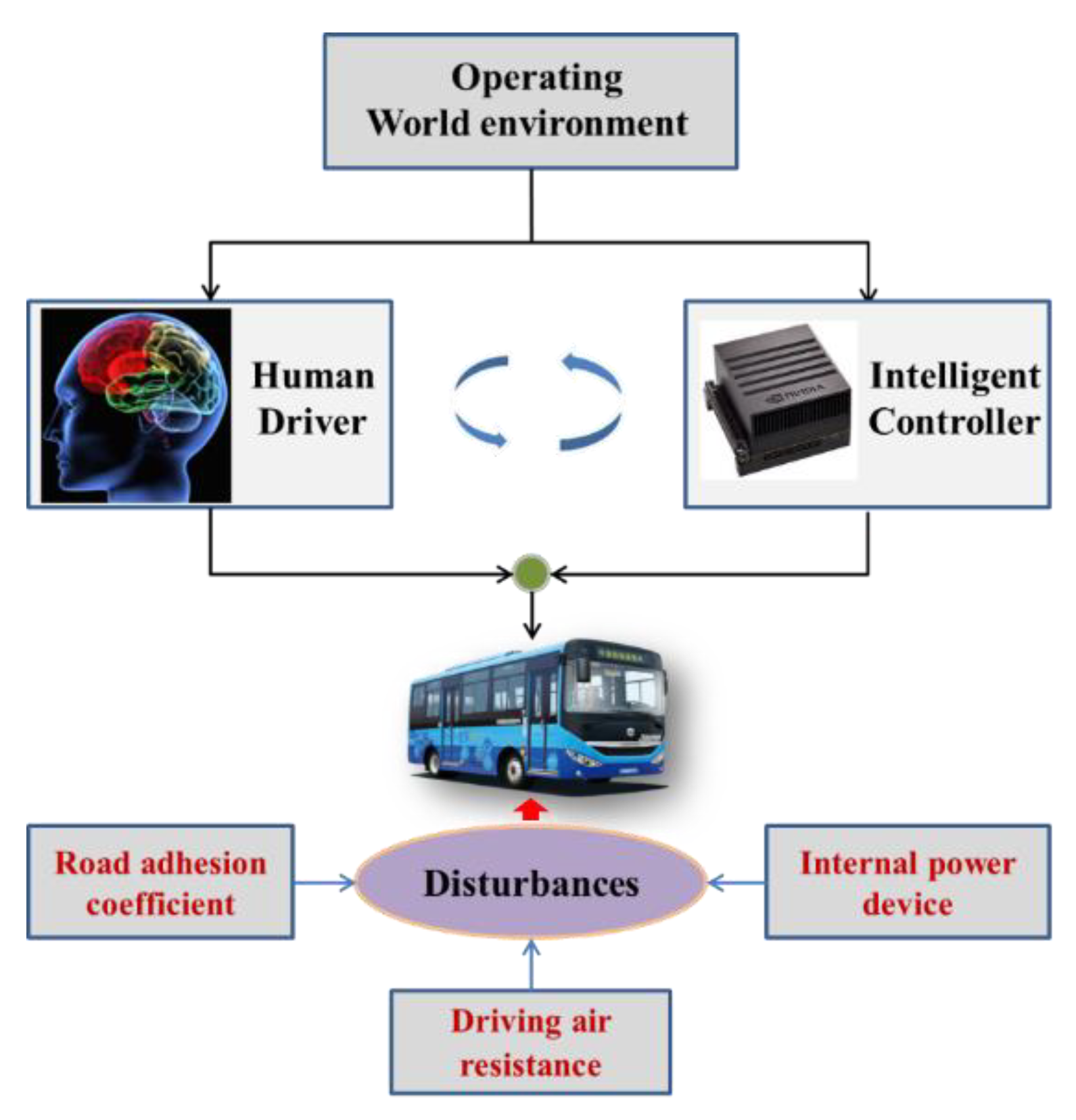
- In this paper, we propose a self-optimized PID controller with a new adaptive updating rule, based on a reinforcement learning framework for autonomous vehicle path tracking control systems, in order to track a predefined path with high accuracy and, simultaneously, provide a comfortable riding experience.
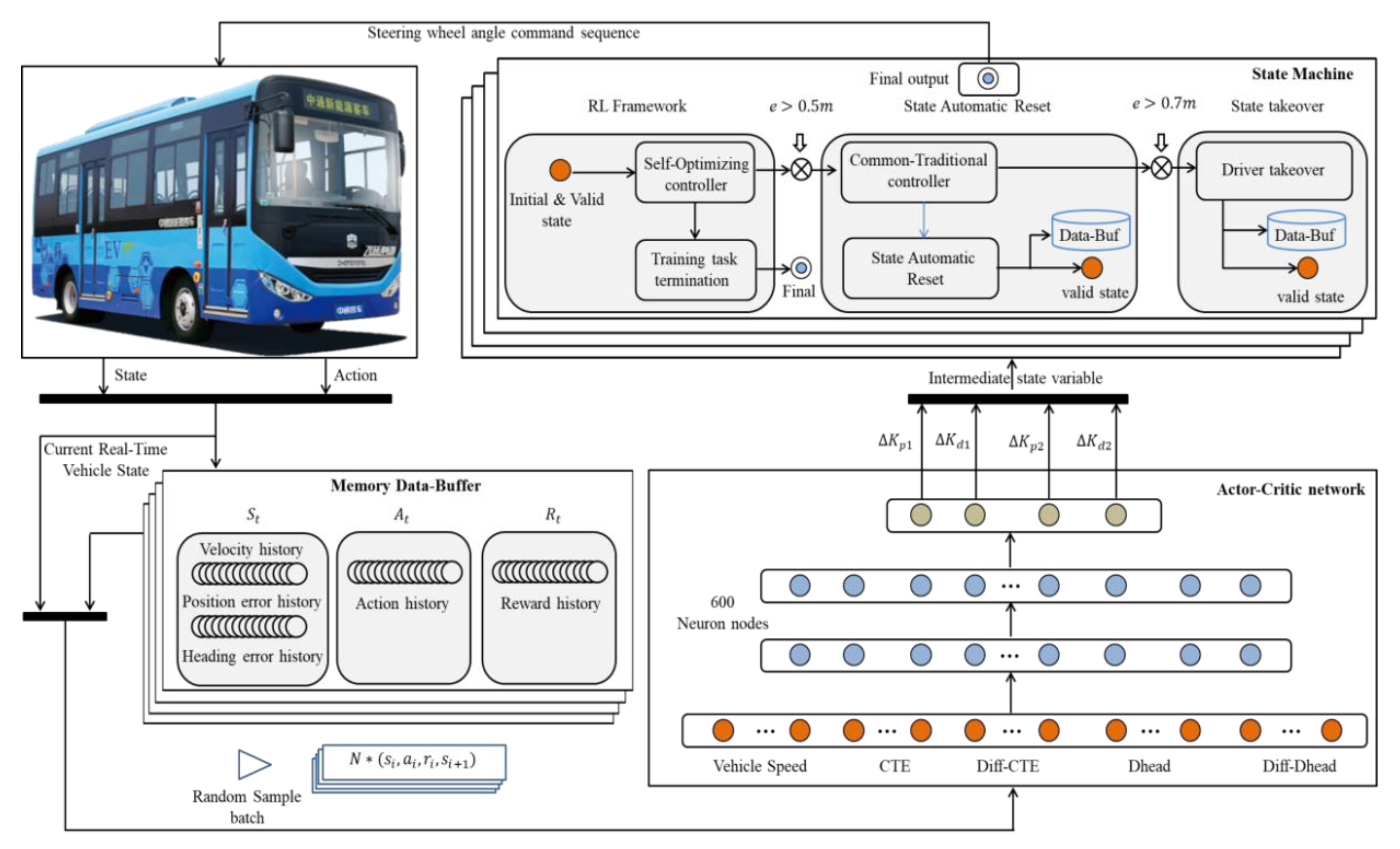
- According to the pre-defined path geometry and the real-time status of the vehicle, the environment interactive learning mechanism, based on RL framework, can realize the online self-tuning of PID control parameters.
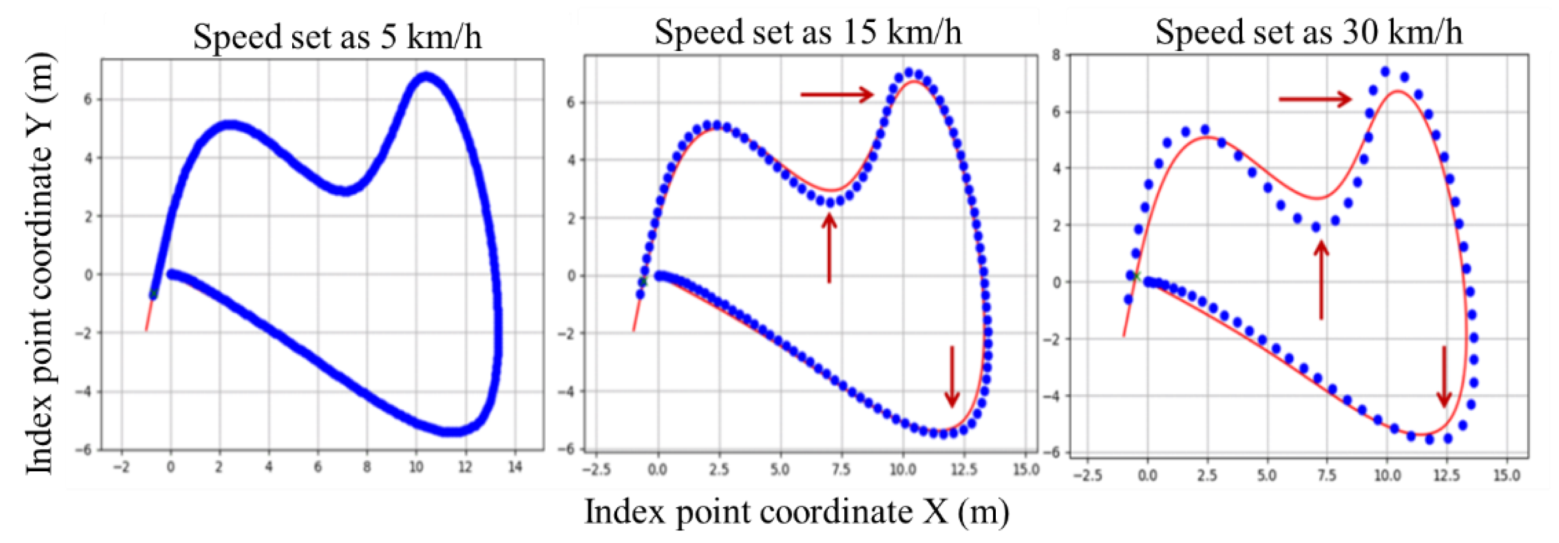
- In order to verify the stability and generalizability of the controller under complex paths and variable speed conditions, the proposed self-optimizing controller was tested in different path tracking scenarios. Finally, a realistic vehicle platform test was carried out to validate the practicability.
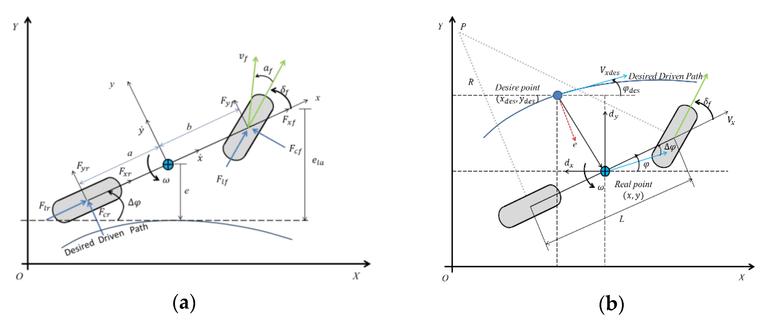
2. Vehicle Dynamic Constraints and Reference Trajectory Generation
- By ignoring the movement in the Z-axis direction, only the movement in the XY horizontal plane is considered; this is referred to as the planar bicycle model.
- By assuming that the rotation angles of the tires on the left and right sides of the vehicle body are identical, the tires on both sides can be combined into one tire.
- The rear wheels are not considered as steering wheels; only the front wheels are.
- The aerodynamic forces are ignored.
- (a)
- State space variable description
- (b)
- Action space variable description
- (c)
- Reward function description
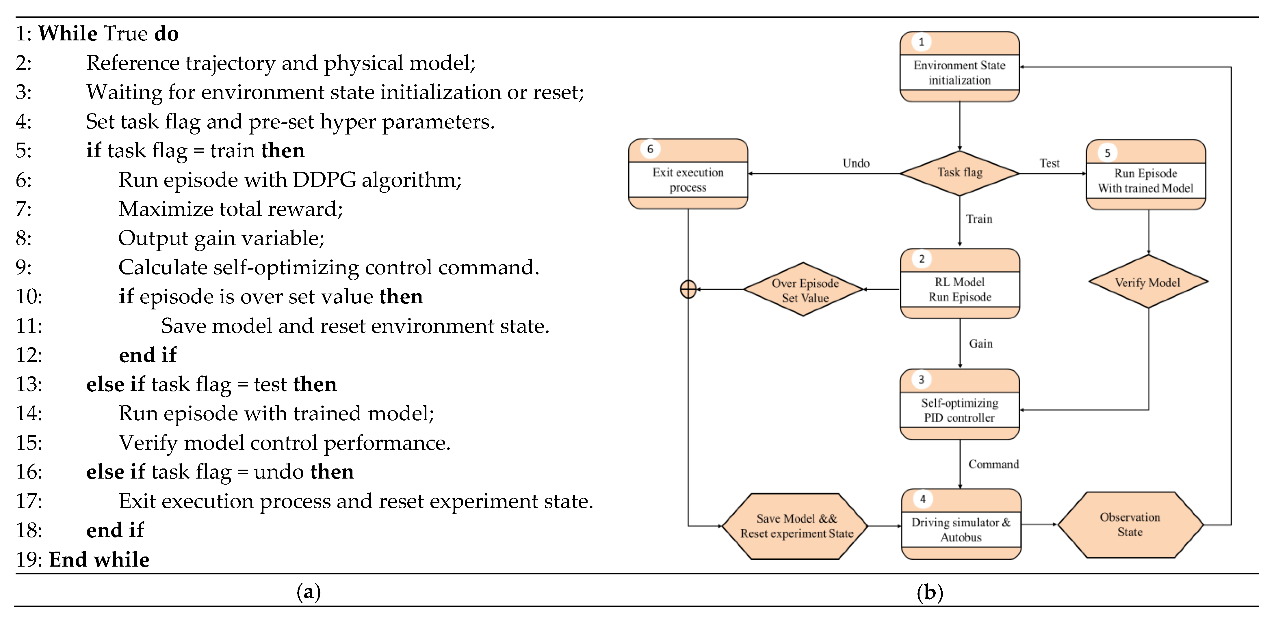
3. Self-Optimizing Path Tracking Controller Based on a Reinforcement Learning (RL) Framework
- (1)
- Initialize the state of the controlled object, including the initial position and heading angle of the vehicle.
- (2)
- Pre-set the parameters for the optimizing controller, including the weight of the actor–critic network, the learning rate, the discount factor, and the selection of the activation function.
- (3)
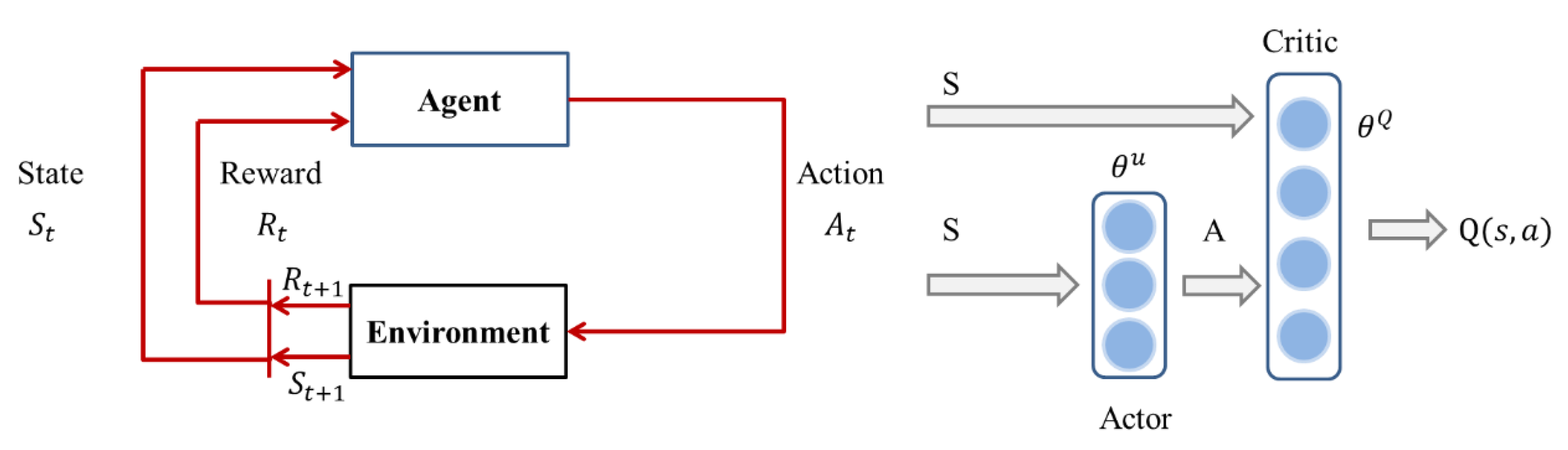
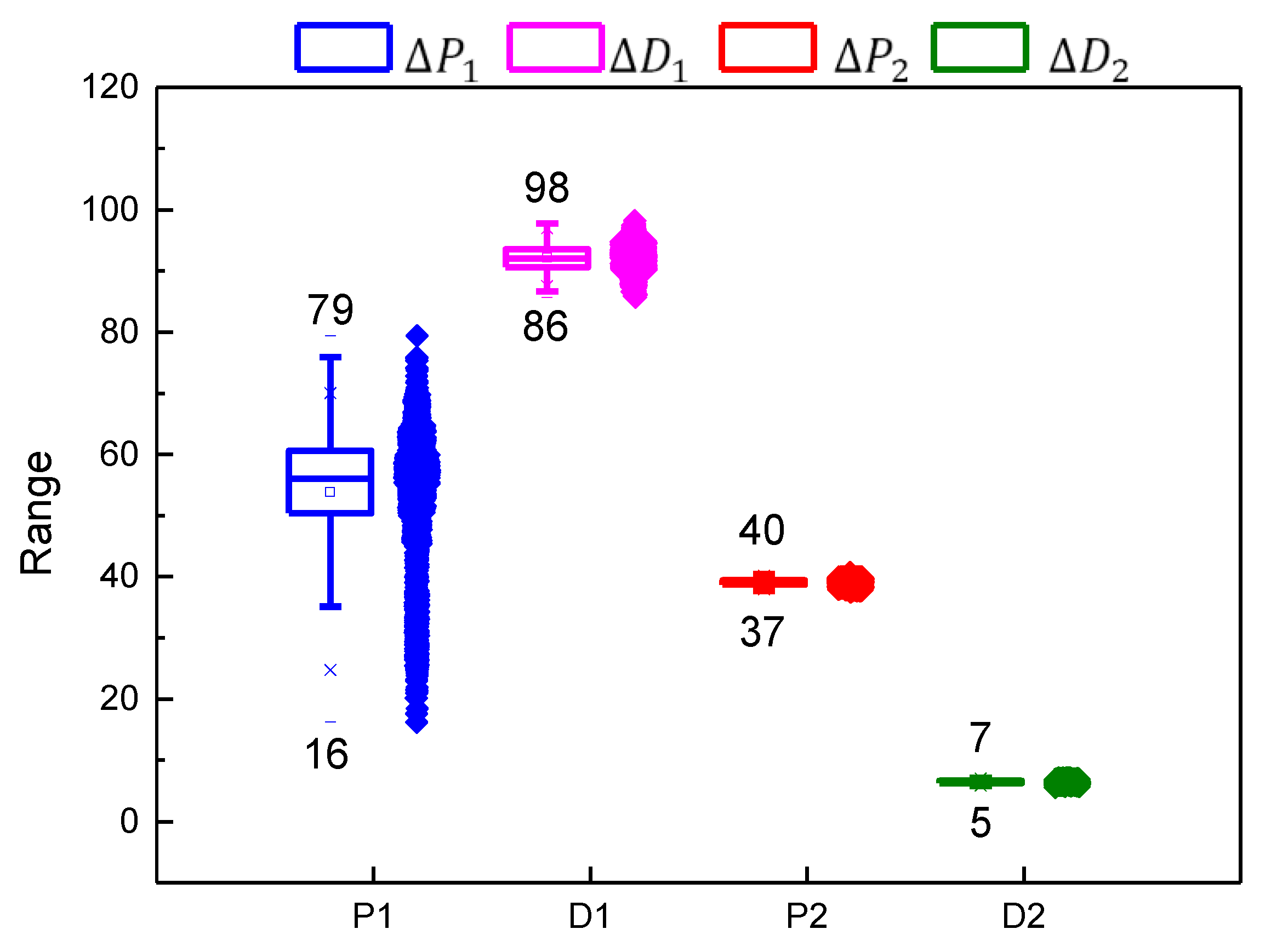
- Adopt the DDPG algorithm to train the model, where the actor network outputs the PID gain, and the critic network maximizes the total reward value.
- (4)
- According to the calculation formula for the self-optimizing PID controller, calculate the control commands.
- (5)
- Use the time series control commands to act on the controlled object, while simultaneously observing the state of the environment at the next moment and calculating the reward function value.
- (6)
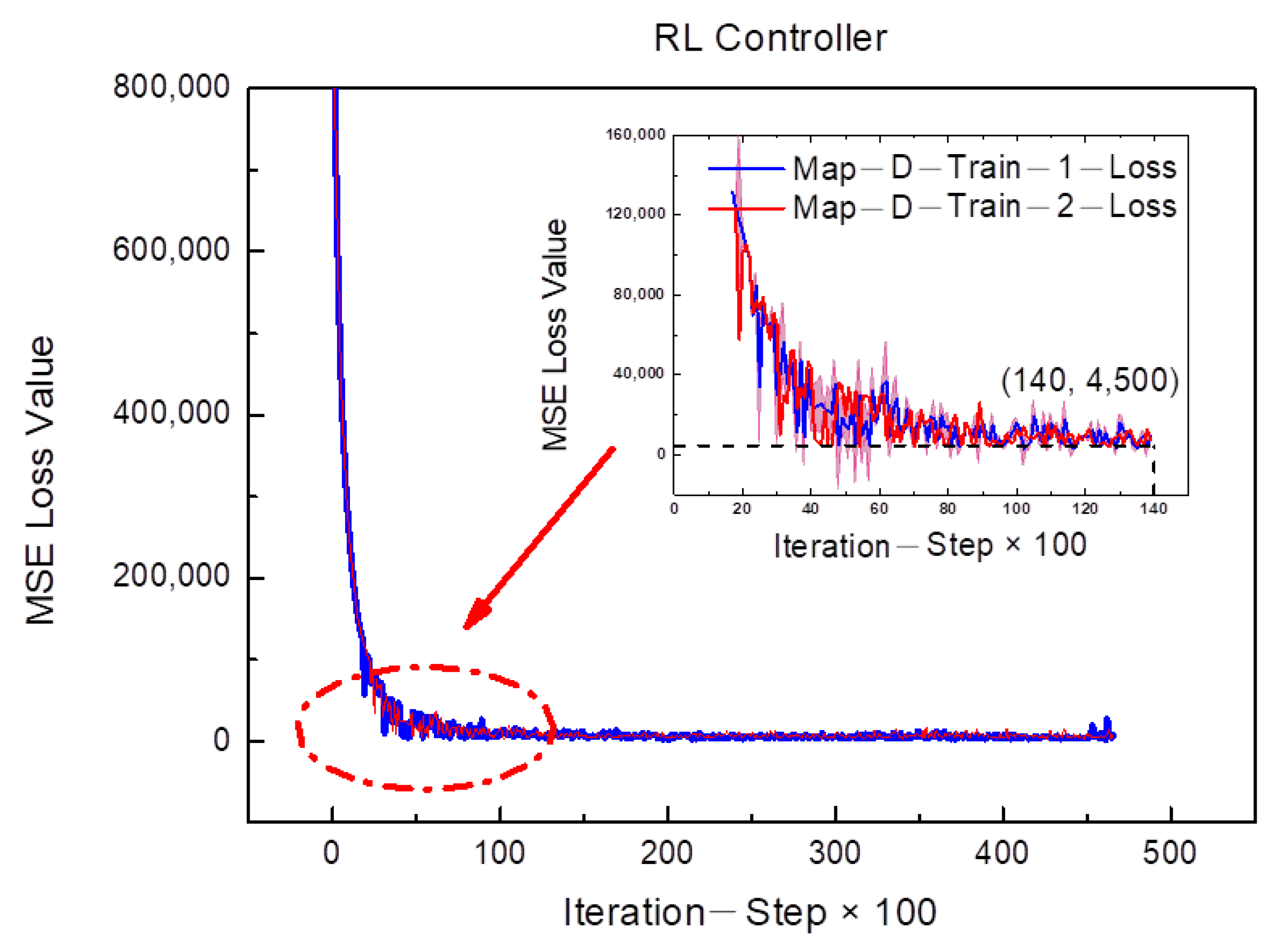
- The actor network uses the DDPG algorithm to update its own weights. The critic network updates its weight, based on the mean squared error (MSE) loss function.
- (7)
- If the system performance indicators meet the given requirements, or the maximum number of run episodes is reached, the training is terminated, the execution process is exited, and the experiment state is reset.
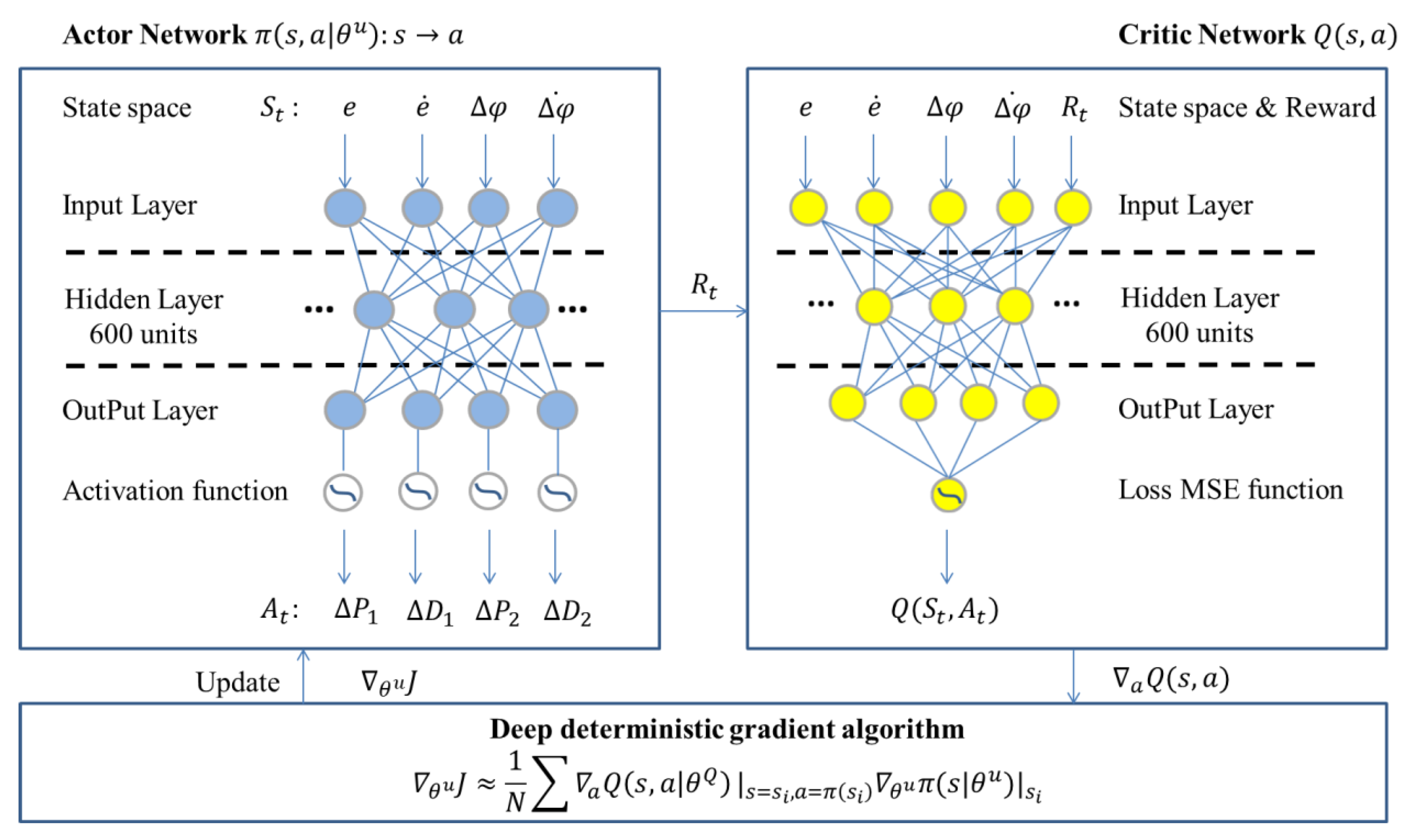
- a.
- Actor–critic network architecture design
- b.
- RL deep deterministic policy gradient (DDPG) algorithm
| Algorithm 1. Pseudo-code programming process of the deterministic policy gradient (DDPG) algorithm |
| Actor uses a gradient algorithm to update the network parameters; Critic uses the mean squared error (MSE) loss function to update the network parameters. Algorithm input: Episode number, T; state dimension, n; action set, A; learning rate, α,β; discount, γ; exploration rate, ; actor–critic network structure; randomly initialize the weighting parameter. |
| Algorithm output: Actor network parameters, , critic network parameters, . |
| 1: for Episode from 1 to (Max Episode -1) do |
| 2: Receive initial observation state, obtain environment state vector . |
| 3: Initialize buffer replay data-buff. |
| 3: for t from 1 to T do |
| 4: Select action . |
| 5: Execute action and observe new state . Calculate instant reward feedback. |
| 6: Store transition in data-buff. |
| 7: Random mini-batch of N transitions from data-buff. |
| 8: Set . 9: Update critic by minimizing MSE loss function: 10: . |
| 11: Update the actor policy using the policy gradient function: 12: . 13: Update the target networks: 14: , 15: . 16: End for time step 17: End for Episode |
4. Experiment and Analysis of Results
4.1. Experimental Setting
- a.
- Simulation experiment platform
- b.
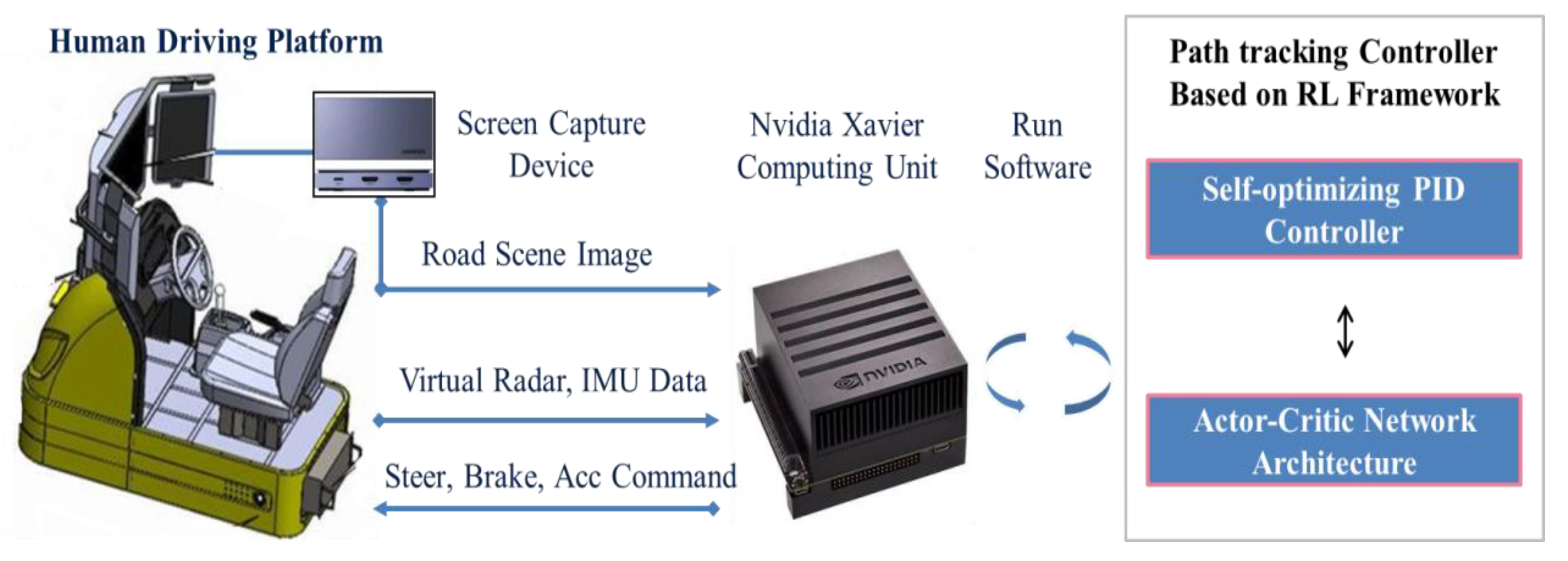
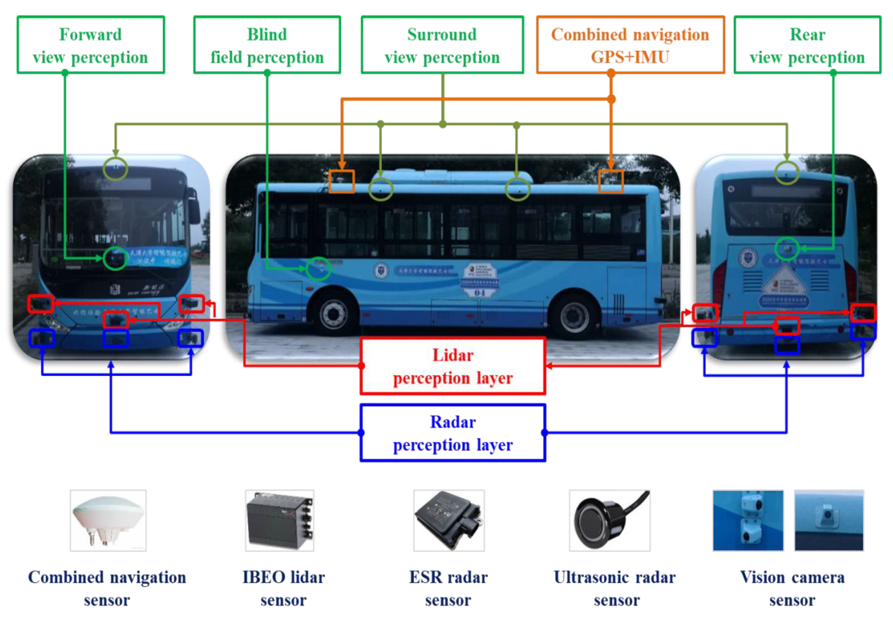
- Realistic autobus experiment platform
- c.
- Software version and hardware computing platform
4.2. Performance Verification and Results Analysis
- a.
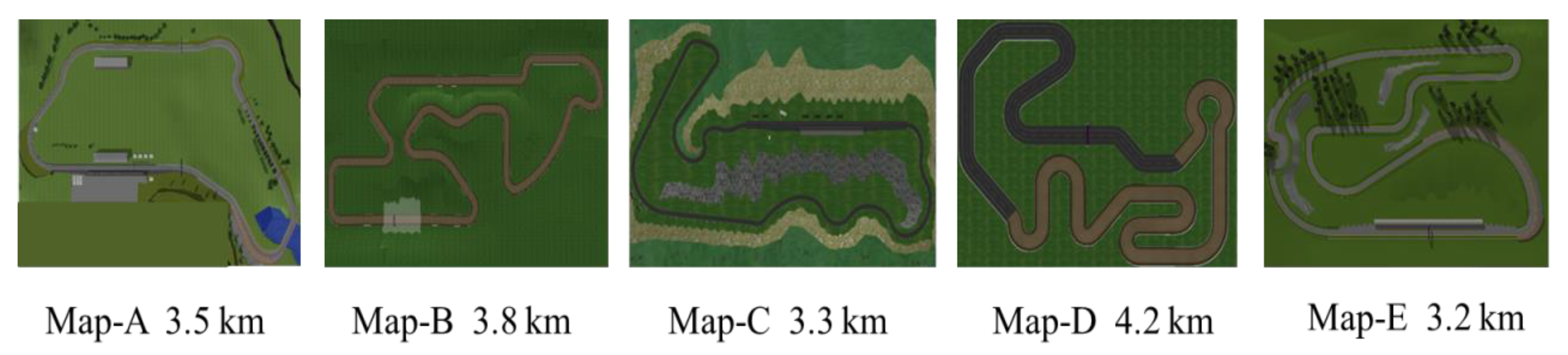
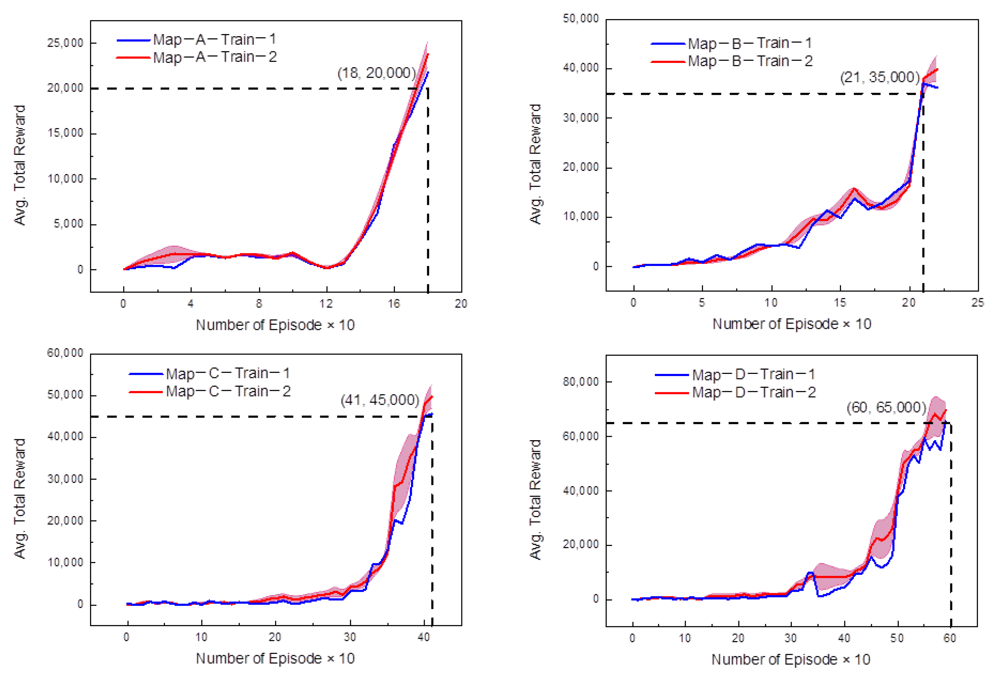
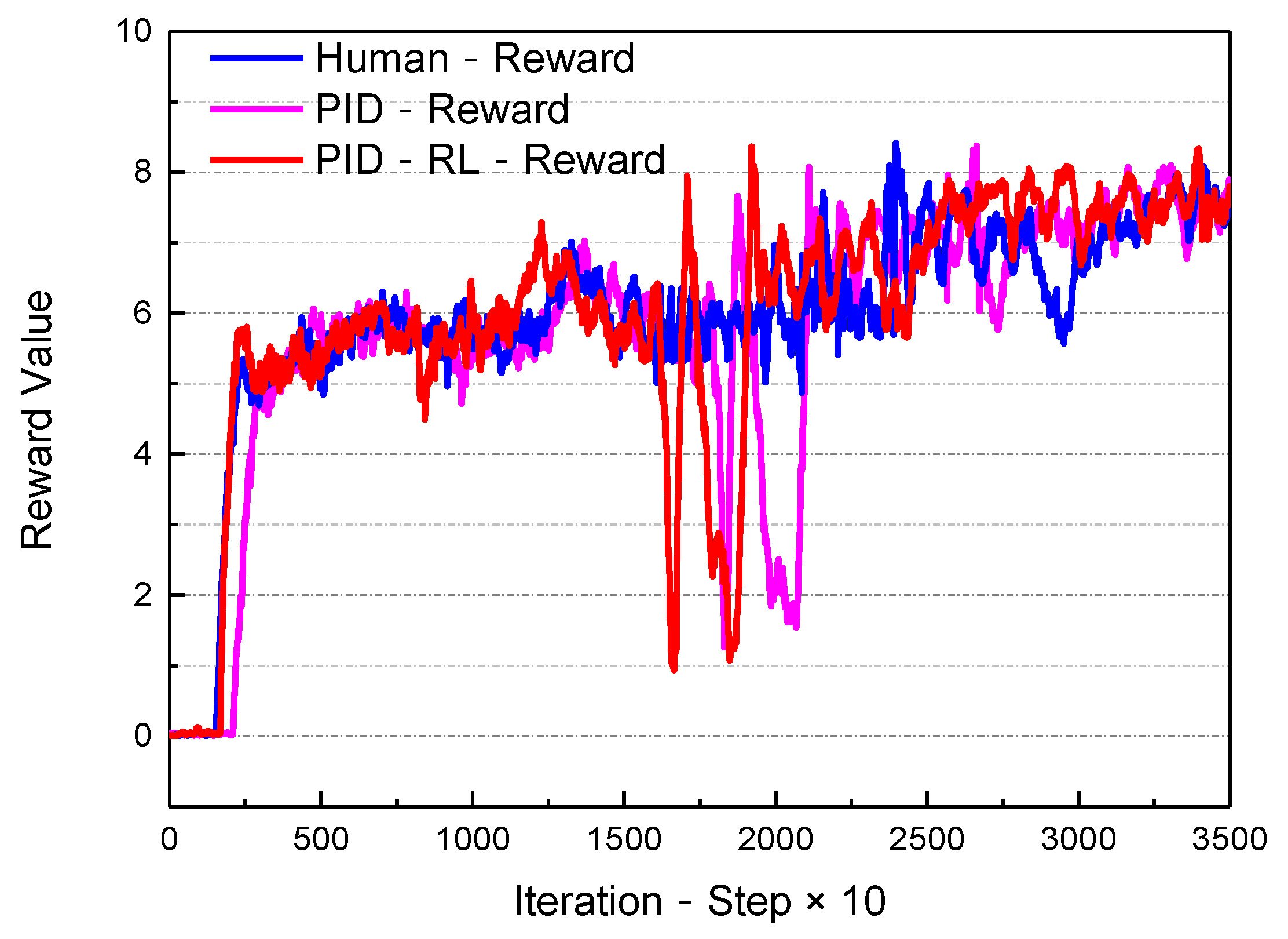
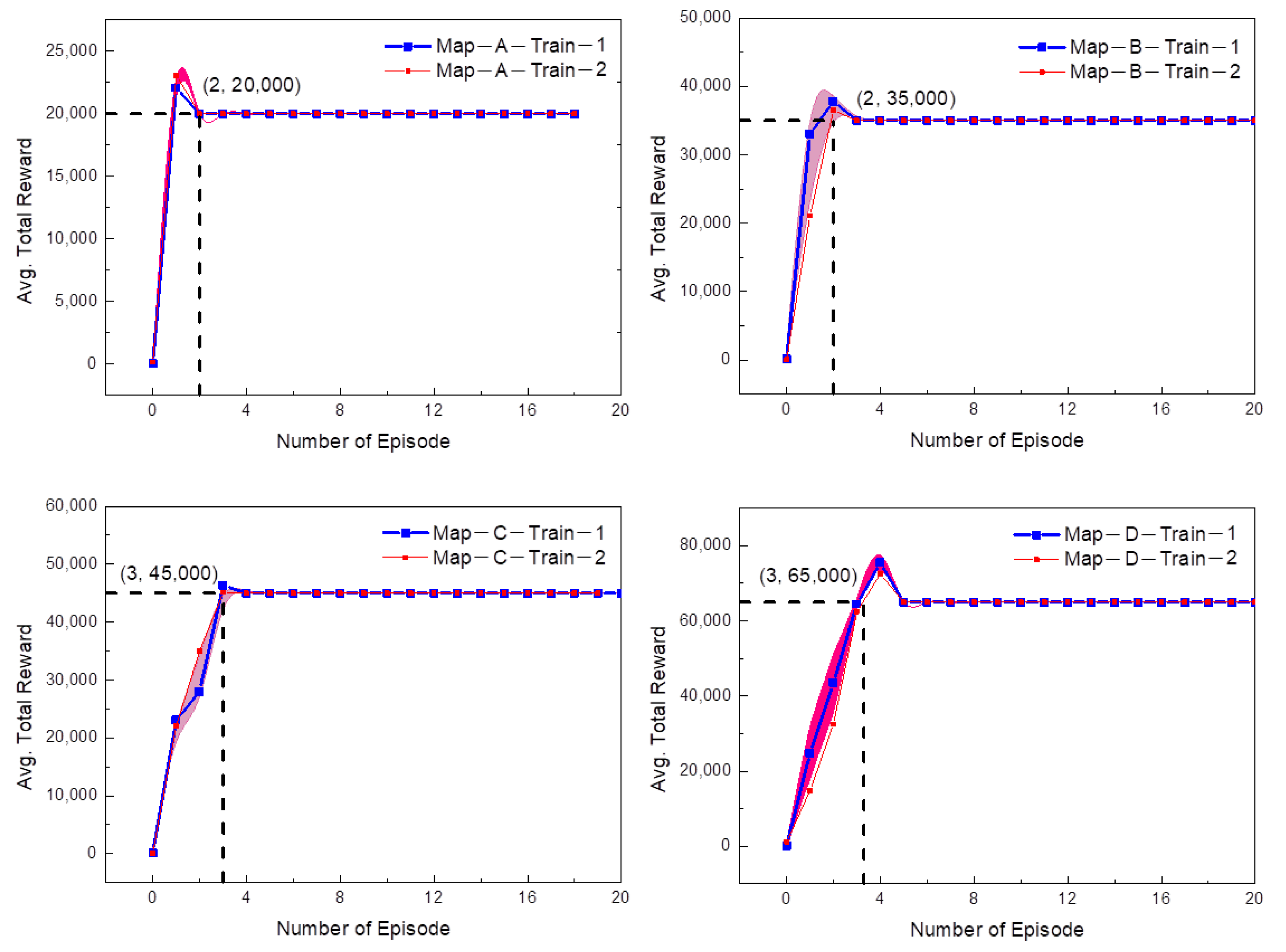
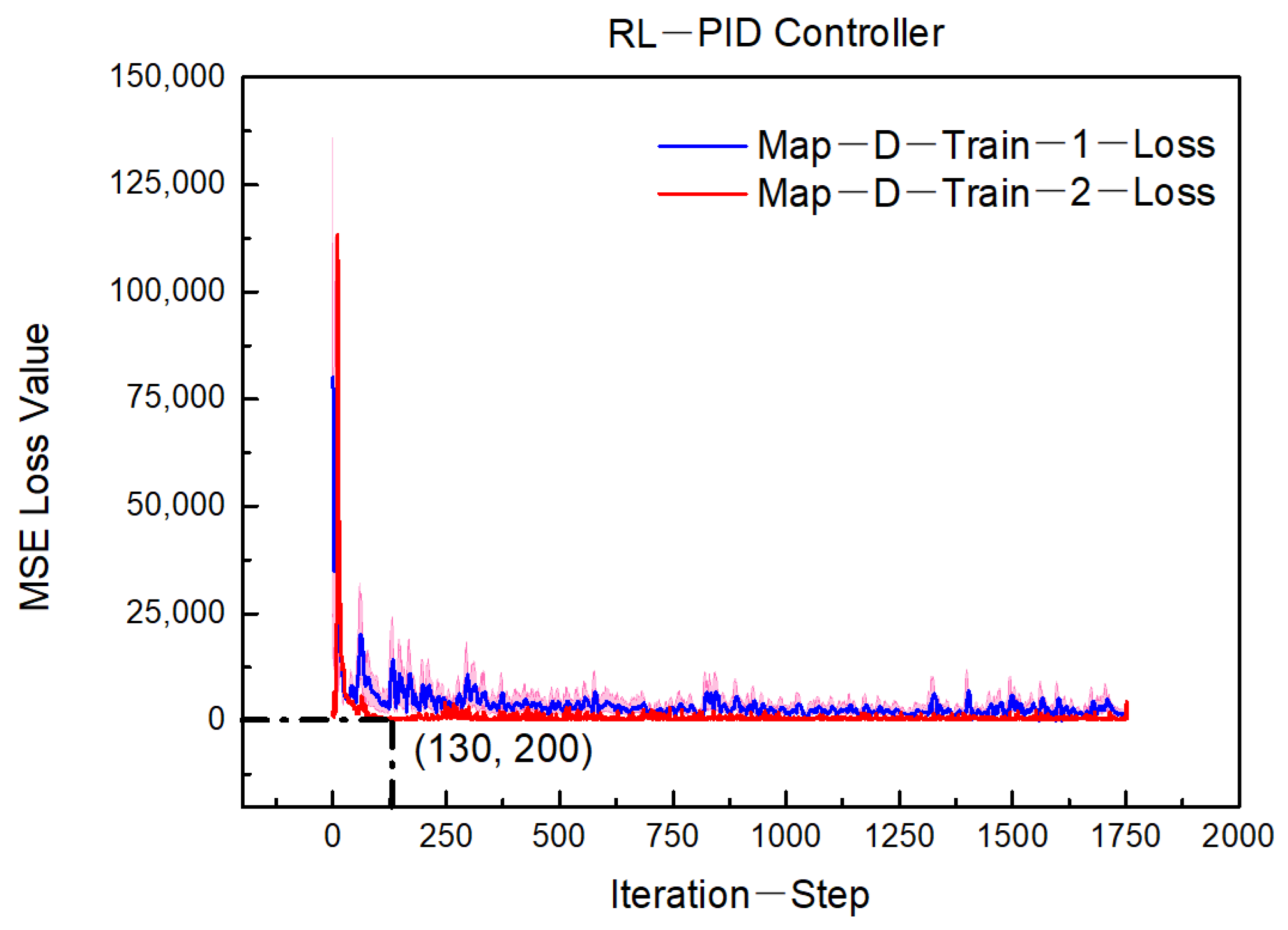
- Simulation experiment setup and performance during training process
- b.
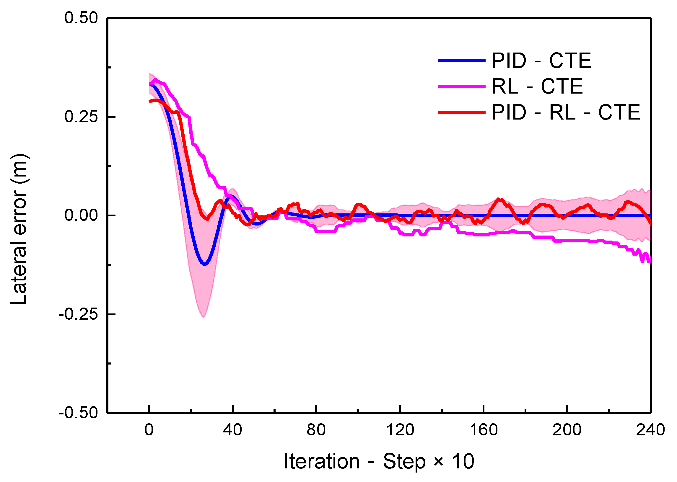
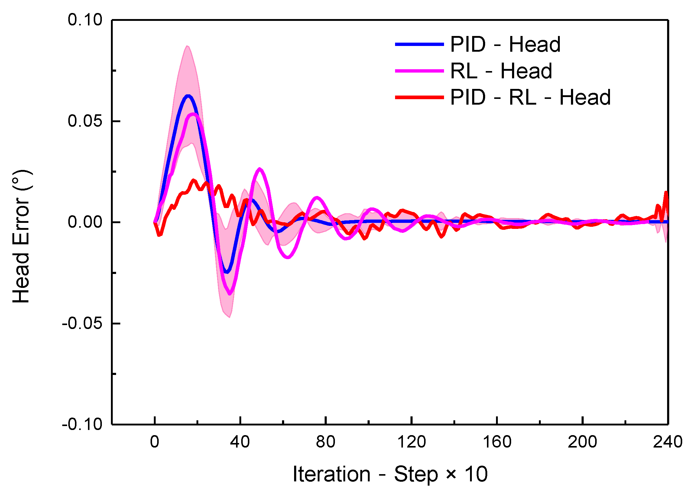
- Evaluating the performance of self-optimizing proportional–integral–derivative (PID) controller, based on RL framework
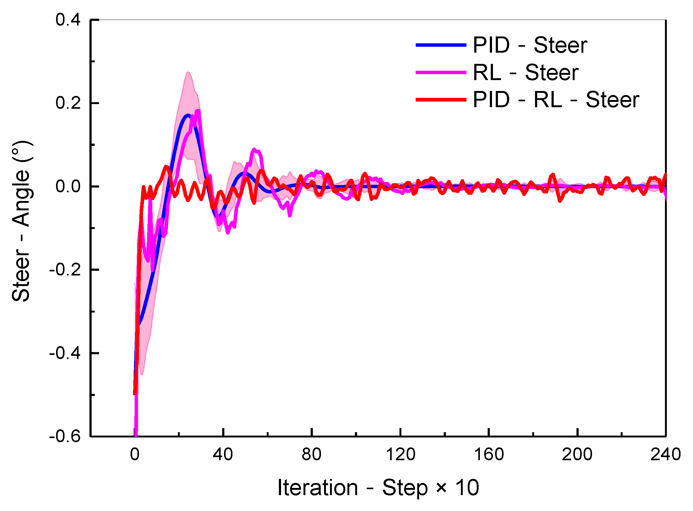
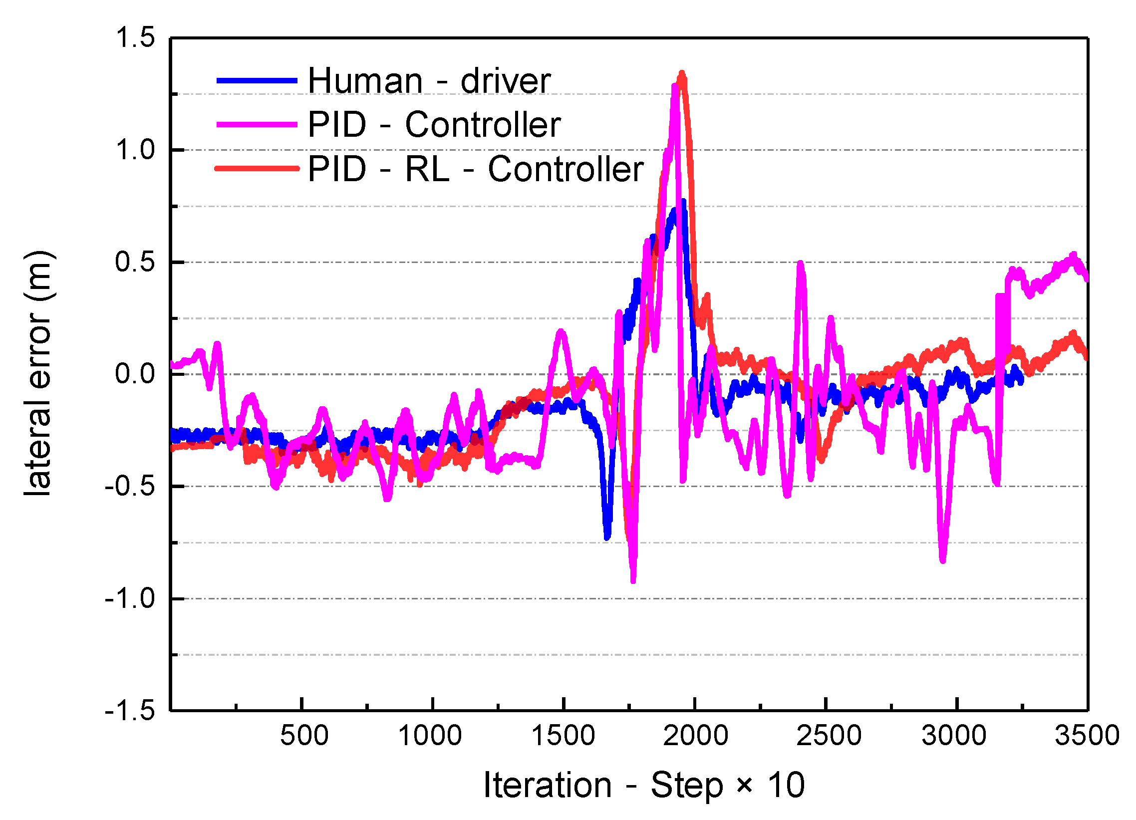
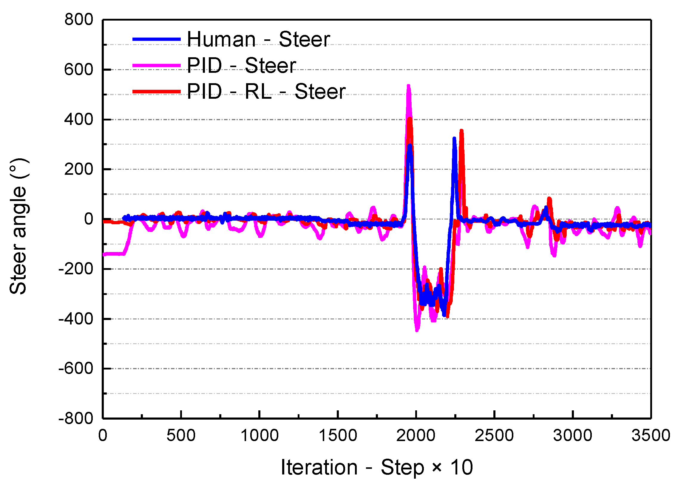
- The smoothness indicator represents the comfort resulting from the path-following control. In this paper, the vibration amplitude of the steering wheel was used to represent the smoothness indicator.
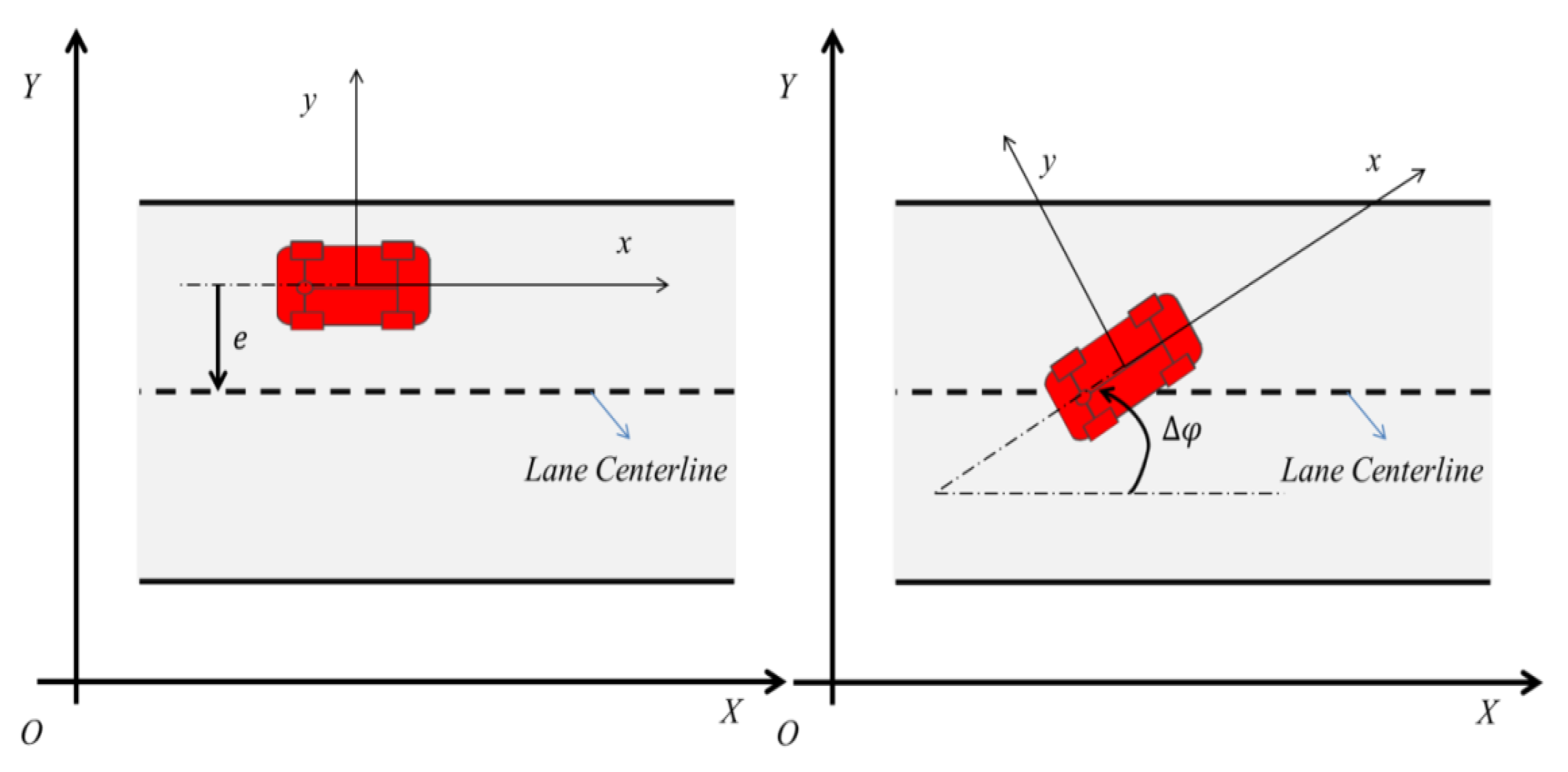
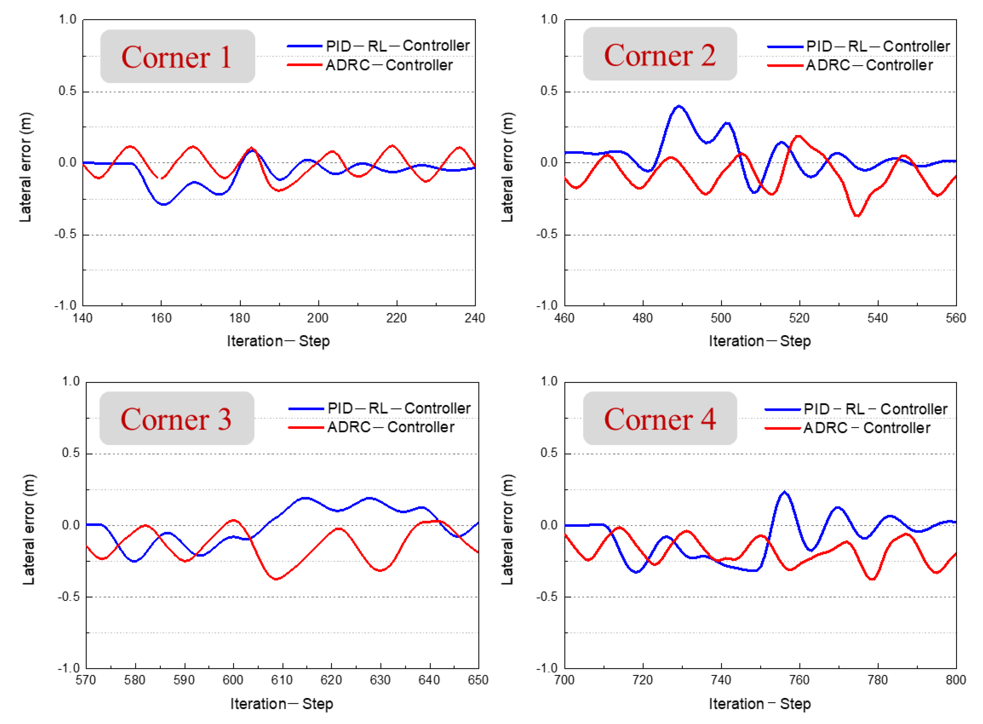
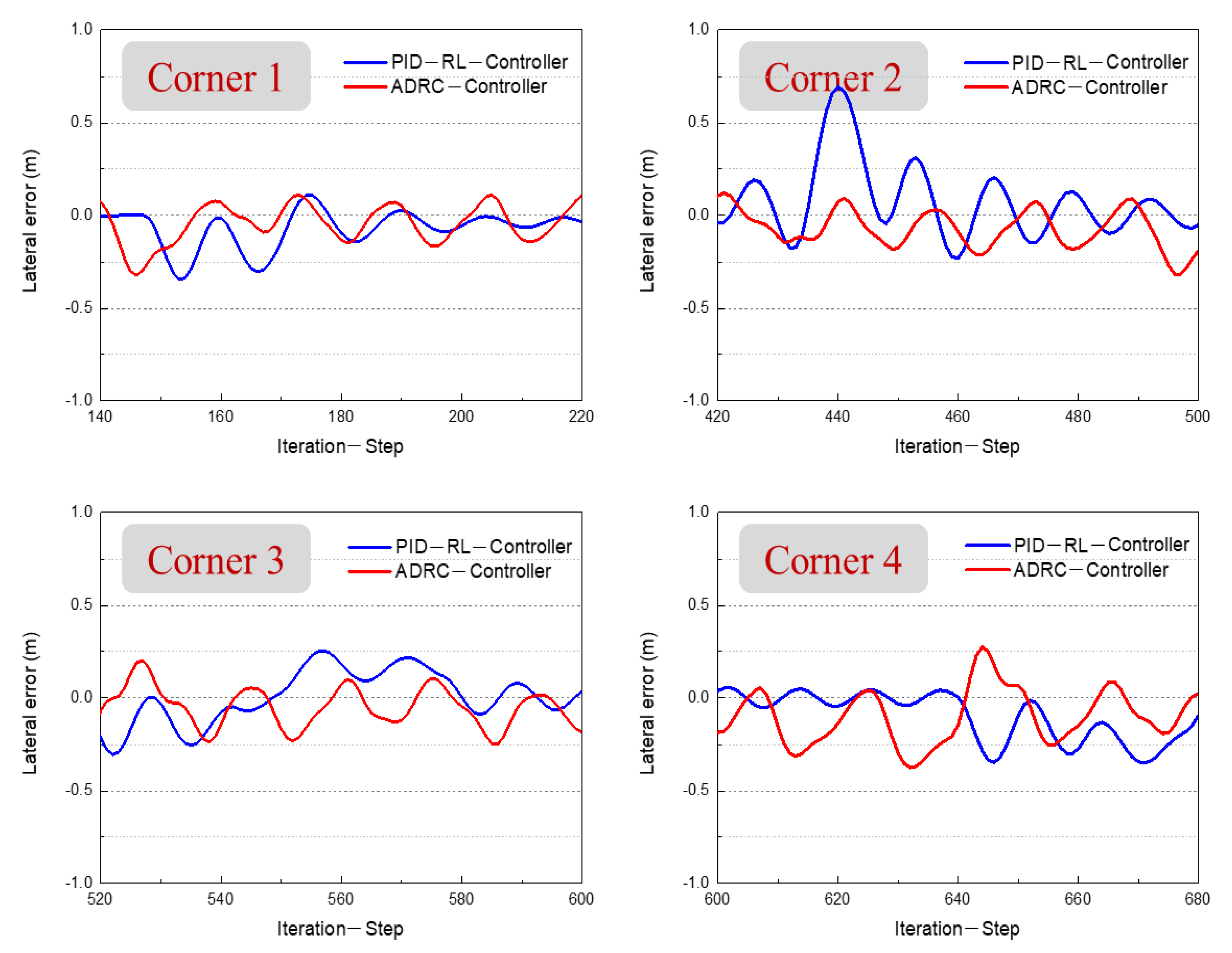
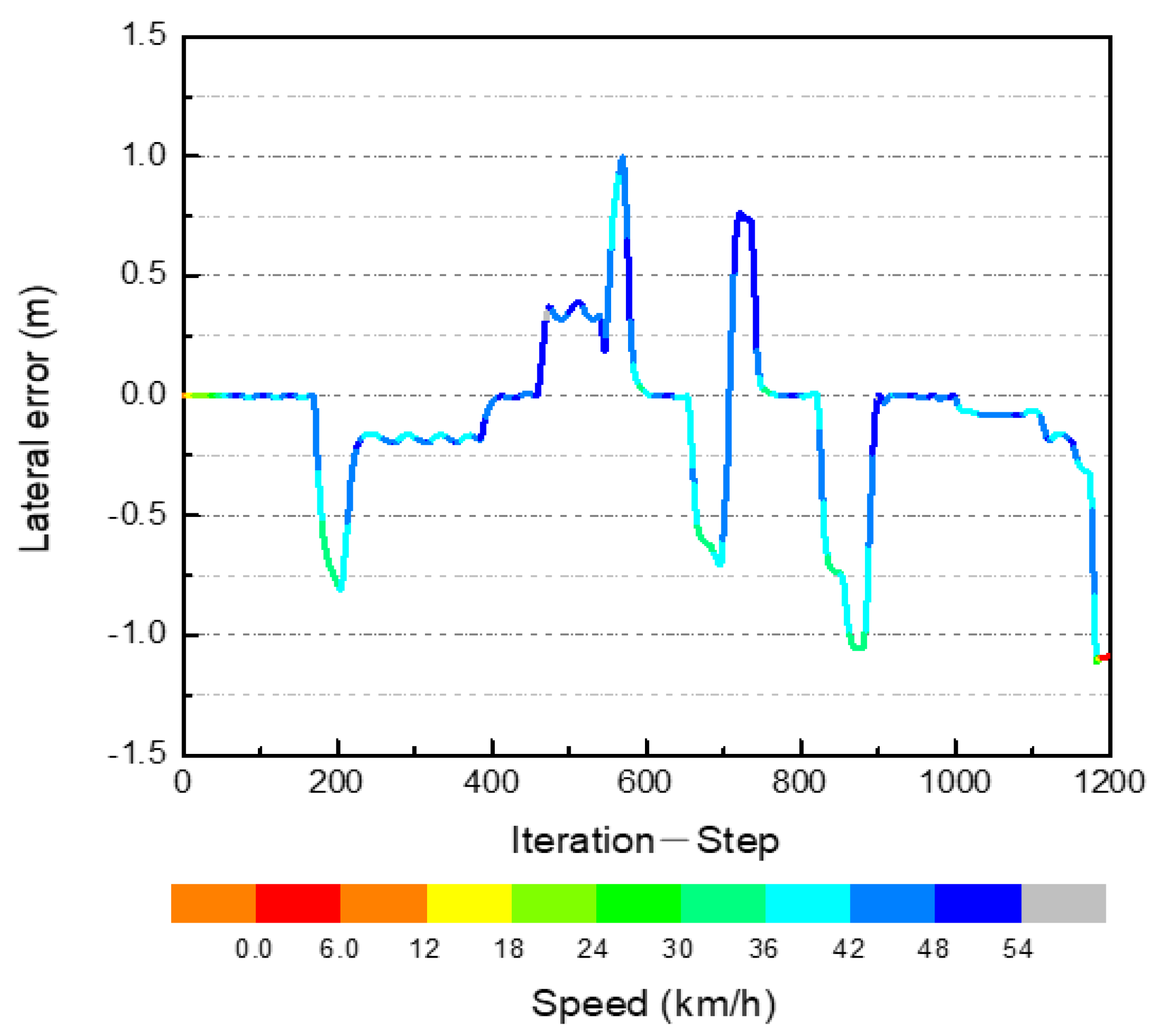
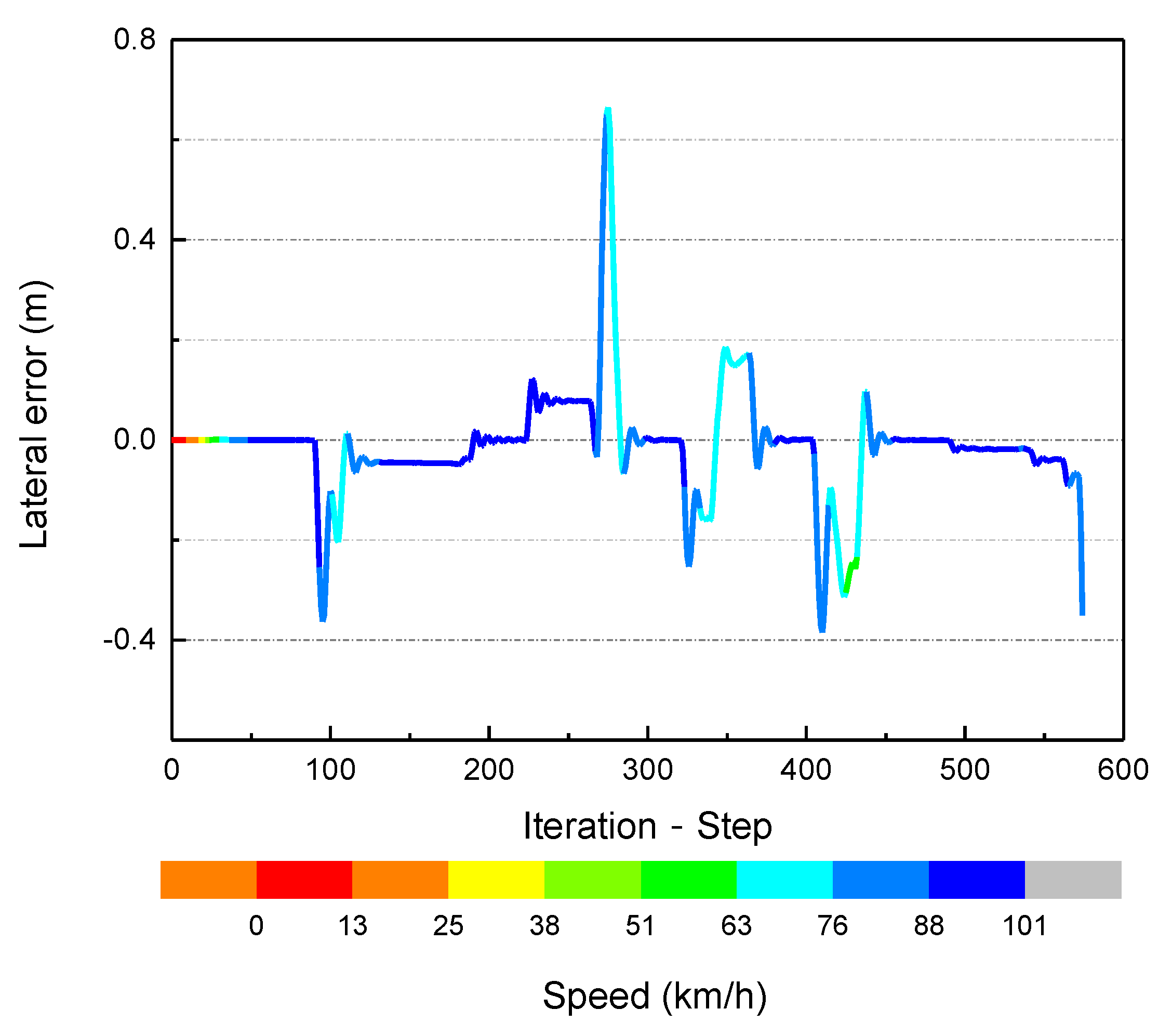
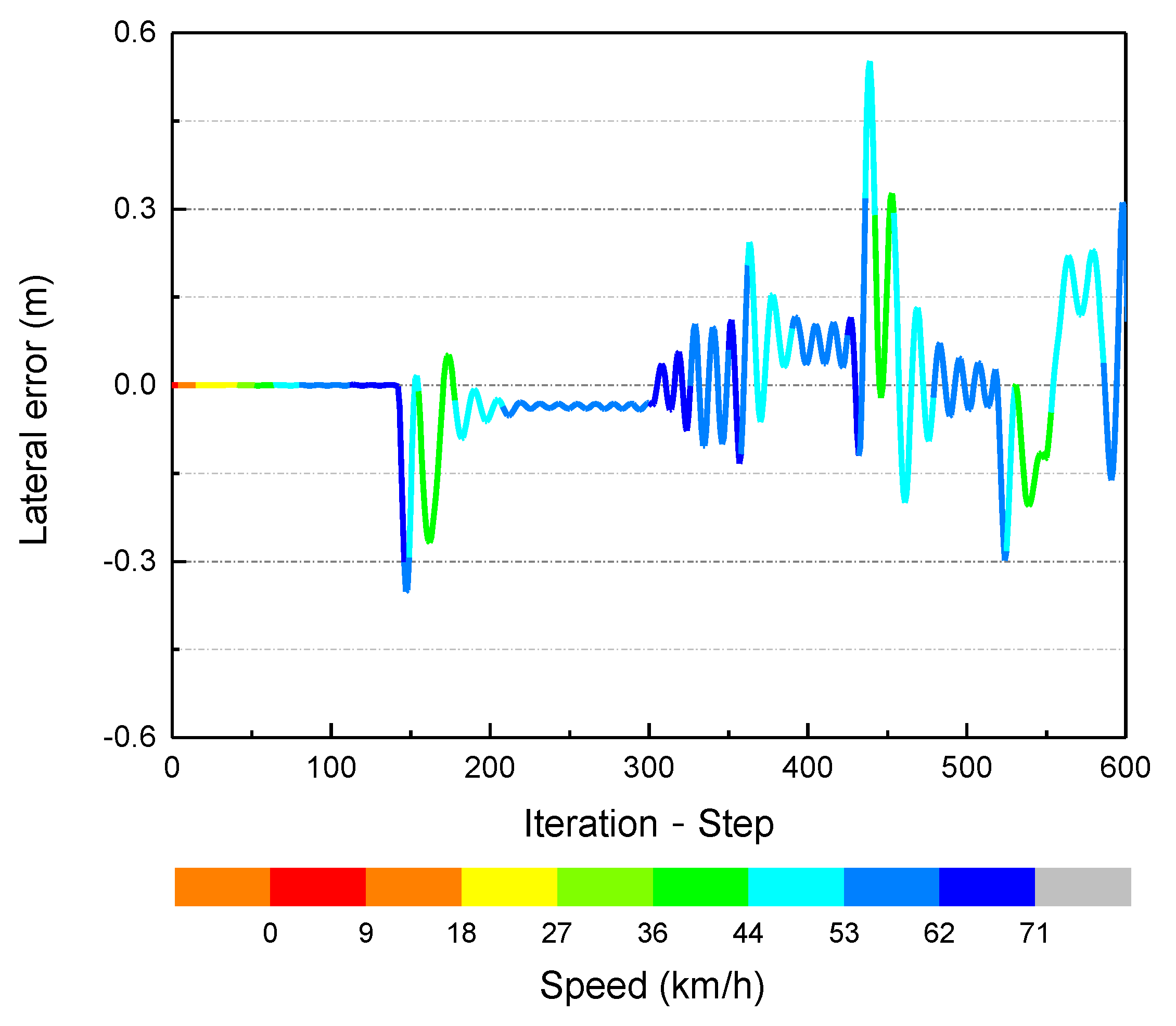
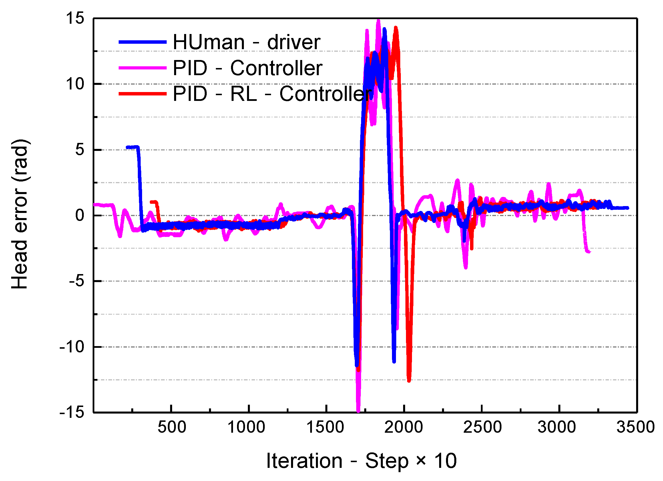
- The lateral track error, , and heading angle error, Δφ, evaluate the effects of the path tracking.
- The maximum speed and average speed indicators characterize the driving efficiency.
- c.
- Generalization of self-optimizing PID controller based on the RL framework
- d.
- Steering of a realistic autobus platform, based on the self-optimizing PID controller
5. Conclusions
6. Discussion of Limitations and Future Work
Author Contributions
Funding
Conflicts of Interest
References
- Visioli, A. Practical PID Control; Springer: Berlin/Heidelberg, Germany, 2006. [Google Scholar]
- Jeffrey, S.; Wit, J.; Crane, C.D., III; Armstrong, D. Autonomous Ground Vehicle Path Tracking; University of Florida: Gainesville, FL, USA, 2000. [Google Scholar]
- Johary, N.M. Path Tracking Algorithm for An Autonomous Ground Robot. Ph.D. Thesis, Universiti Tun Hussein Onn Malaysia, Batu Pahat, Malaysia, 2014. [Google Scholar]
- Goh, J.Y.; Goel, T.; Gerdes, J.C. A controller for automated drifting along complex trajectories. In Proceedings of the 14th International Symposium on Advanced Vehicle Control (AVEC 2018), Beijing, China, 16–20 July 2018. [Google Scholar]
- Goh, J.Y.; Gerdes, J.C. Simultaneous stabilization and tracking of basic automobile drifting trajectories. In Proceedings of the 2016 IEEE Intelligent Vehicles Symposium (IV), Los Angeles, CA, USA, 11–14 June 2017; pp. 597–602. [Google Scholar]
- Hindiyeh, R.Y.; Gerdes, J.C. A controller framework for autonomous drifting: Design, stability, and experimental validation. J. Dyn. Syst. Meas. Control. 2014, 136, 051015. [Google Scholar] [CrossRef]
- Kim, D.; Yi, K. Design of a Path for Collision Avoidance and Path Tracking Scheme for Autonomous Vehicles. IFAC Proc. Vol. 2009, 42, 391–398. [Google Scholar] [CrossRef]
- Chen, S.-P.; Xiong, G.-M.; Chen, H.-Y.; Negrut, D. MPC-based path tracking with PID speed control for high-speed autonomous vehicles considering time-optimal travel. J. Central South Univ. 2020, 27, 3702–3720. [Google Scholar] [CrossRef]
- Wang, H.; Liu, B.; Ping, X.; An, Q. Path Tracking Control for Autonomous Vehicles Based on an Improved MPC. IEEE Access 2019, 7, 161064–161073. [Google Scholar] [CrossRef]
- Kim, D.; Kang, J.; Yi, K. Control strategy for high-speed autonomous driving in structured road. In Proceedings of the 2011 14th International IEEE Conference on Intelligent Transportation Systems (ITSC), Washington, DC, USA, 5–7 October 2011. [Google Scholar]
- Vivek, K.; Sheta, M.A.; Gumtapure, V. A Comparative Study of Stanley, LQR and MPC Controllers for Path Tracking Application (ADAS/AD). In Proceedings of the 2019 IEEE International Conference on Intelligent Systems and Green Technology (ICISGT), Visakhapatnam, India, 29–30 June 2019. [Google Scholar]
- Tiep, D.K.; Lee, K.; Im, D.-Y.; Kwak, B.; Ryoo, Y.-J. Design of Fuzzy-PID Controller for Path Tracking of Mobile Robot with Differential Drive. Int. J. Fuzzy Log. Intell. Syst. 2018, 18, 220–228. [Google Scholar] [CrossRef]
- El Hamidi, K.; Mjahed, M.; El Kari, A.; Ayad, H. Neural Network and Fuzzy-logic-based Self-tuning PID Control for Quadcopter Path Tracking. Stud. Inform. Control 2019, 28, 401–412. [Google Scholar] [CrossRef]
- Liang, X.; Zhang, W.; Wu, Y. Automatic Collimation of Optical Path Based on BP-PID Control. In Proceedings of the 2017 10th International Conference on Intelligent Computation Technology and Automation (ICICTA), Changsha, China, 9–10 October 2017. [Google Scholar]
- Ma, L.; Yao, Y.; Wang, M. The Optimizing Design of Wheeled Robot Tracking System by PID Control Algorithm Based on BP Neural Network. In Proceedings of the 2016 International Conference on Industrial Informatics-Computing Technology, Wuhan, China, 3–4 December 2016. [Google Scholar]
- El Sallab, A.; Abdou, M.; Perot, E.; Yogamani, S. Deep Reinforcement Learning framework for Autonomous Driving. Electron. Imaging 2017, 2017, 70–76. [Google Scholar] [CrossRef] [Green Version]
- Wang, S.; Jia, D.; Weng, X. Deep Reinforcement Learning for Autonomous Driving. arXiv 2018, arXiv:1811.11329. [Google Scholar]
- Dong, L.; Zhao, D.; Zhang, Q.; Chen, Y. Reinforcement Learning and Deep Learning based Lateral Control for Autonomous Driving. arXiv 2018, arXiv:1810.12778. [Google Scholar]
- Wymann, B.; Espié, E.; Guionneau, C.; Dimitrakakis, C.; Coulom, R.; Sumner, A. TORCS, The Open Racing Car Simulator, v1.3.5. 2013. Available online: http://torcs.sourceforge.net/ (accessed on 10 December 2019).
- Ingram, A. Gran Turismo Sport—Exploring Its Impact on Real-World Racing with Kazunori. 2019. Available online: Yamauchi.evo.co.uk (accessed on 1 June 2020).
- Fuchs, F.; Song, Y.; Kaufmann, E.; Scaramuzza, D.; Dürr, P. Super-Human Performance in Gran Turismo Sport Using Deep Reinforcement Learning. arXiv 2020, arXiv:2008.07971. [Google Scholar] [CrossRef]
- Cai, P.; Mei, X.; Tai, L.; Sun, Y.; Liu, M. High-Speed Autonomous Drifting With Deep Reinforcement Learning. IEEE Robot. Autom. Lett. 2020, 5, 1247–1254. [Google Scholar] [CrossRef] [Green Version]
- Dosovitskiy, A.; Ros, G.; Codevilla, F.; Lopez, A.; Koltun, V. Carla: An open urban driving simulator. arXiv 2017, arXiv:1711.03938. [Google Scholar]
- Gao, X.; Gao, R.; Liang, P.; Zhang, Q.; Deng, R.; Zhu, W. A Hybrid Tracking Control Strategy for Nonholonomic Wheeled Mobile Robot Incorporating Deep Reinforcement Learning Approach. IEEE Access 2021, 9, 15592–15602. [Google Scholar] [CrossRef]
- Zhang, Y.; Zhang, Y.; Yu, Z. Path Following Control for UAV Using Deep Reinforcement Learning Approach. Guid. Navig. Control 2021, 1, 2150005. [Google Scholar] [CrossRef]
- Duan, K.; Fong, S.; Chen, C.P. Reinforcement Learning Based Model-free Optimized Trajectory Tracking Strategy Design for an AUV. Neurocomputing 2022, 469, 289–297. [Google Scholar] [CrossRef]
- Li, B.; Wu, Y. Path Planning for UAV Ground Target Tracking via Deep Reinforcement Learning. IEEE Access 2020, 8, 29064–29074. [Google Scholar] [CrossRef]
- Wang, S.; Yin, X.; Li, P.; Zhang, M.; Wang, X. Trajectory Tracking Control for Mobile Robots Using Reinforcement Learning and PID. Iran. J. Sci. Technol. Trans. Electr. Eng. 2020, 44, 1059–1068. [Google Scholar] [CrossRef]
- Xiao, J.; Li, L.; Zou, Y.; Zhang, T. Reinforcement Learning for Robotic Time-optimal Path Tracking Using Prior Knowledge. arXiv 2019, arXiv:1907.00388. [Google Scholar]
- Zhang, S.; Wang, W. Tracking Control for Mobile Robot Based on Deep Reinforcement Learning. In Proceedings of the 2019 2nd International Conference on Intelligent Autonomous Systems (ICoIAS), Singapore, 28 February–2 March 2019. [Google Scholar]
- Arroyo, M.A.; Giraldo, L.F. Data-driven Outer-Loop Control Using Deep Reinforcement Learning for Trajectory Tracking. arXiv 2020, arXiv:2008.13732. [Google Scholar]
- Shan, Y.; Zheng, B.; Chen, L.; Chen, L.; Chen, D. A Reinforcement Learning-Based Adaptive Path Tracking Approach for Autonomous Driving. IEEE Trans. Veh. Technol. 2020, 69, 10581–10595. [Google Scholar] [CrossRef]
- Puccetti, L.; Köpf, F.; Rathgeber, C.; Hohmann, S. Speed Tracking Control using Online Reinforcement Learning in a Real Car. In Proceedings of the 6th IEEE International Conference on Control, Automation and Robotics (ICCAR), Singapore, 20–23 April 2020. [Google Scholar]
- Wang, N.; Gao, Y.; Yang, C.; Zhang, X. Reinforcement Learning-based Finite-time Tracking Control of an Unknown Unmanned Surface Vehicle with Input Constraints. Neurocomputing 2021. Available online: https://www.sciencedirect.com/science/article/abs/pii/S0925231221015733 (accessed on 10 June 2021). [CrossRef]
- Jiang, L.; Wang, Y.; Wang, L.; Wu, J. Path tracking control based on Deep reinforcement learning in Autonomous driving. In Proceedings of the 2019 3rd Conference on Vehicle Control and Intelligence (CVCI), Hefei, China, 21–22 September 2019. [Google Scholar]
- Kamran, D.; Zhu, J.; Lauer, M. Learning Path Tracking for Real Car-like Mobile Robots From Simulation. In Proceedings of the 2019 European Conference on Mobile Robots (ECMR), Prague, Czech Republic, 4–6 September 2019. [Google Scholar]
- Riedmiller, M.; Montemerlo, M.; Dahlkamp, H. Learning to Drive a Real Car in 20 Minutes. In Proceedings of the Frontiers in the Convergence of Bioscience & Information Technologies IEEE Computer Society, Jeju City, Korea, 11–13 October 2007. [Google Scholar]
- Kendall, A.; Hawke, J.; Janz, D.; Mazur, P.; Reda, D.; Allen, J.-M.; Lam, V.-D.; Bewley, A.; Shah, A. Learning to Drive in a Day. arXiv 2018, arXiv:1807.00412. [Google Scholar]
- Rajamani, R. Vehicle Dynamics and Control; Springer Science & Business Media: Berlin/Heidelberg, Germany, 2011. [Google Scholar]
- Kong, J.; Pfeiffer, M.; Schildbach, G.; Borrelli, F. Kinematic and dynamic vehicle models for autonomous driving control design. In Proceedings of the 2015 IEEE Intelligent Vehicles Symposium (IV), Seoul, Korea, 29 June–1 July 2015. [Google Scholar]
- Zhu, M.; Wang, X.; Wang, Y. Human-like autonomous car-following model with deep reinforcement learning. Transp. Res. Part C Emerg. Technol. 2018, 97, 348–368. [Google Scholar] [CrossRef] [Green Version]
- Kingma, D.P.; Ba, J. Adam: A method for stochastic optimization. arXiv 2014, arXiv:1412.6980. [Google Scholar]
- Lillicrap, T.P.; Hunt, J.J.; Pritzel, A.; Heess, N.; Erez, T.; Tassa, Y.; Silver, D.; Wierstra, D. Continuous control with deep reinforcement learning. arXiv 2015, arXiv:1509.02971. [Google Scholar]
- Yu, A.; Palefsky-Smith, R.; Bedi, R. Course Project Reports: Deep Reinforcement Learning for Simulated Autonomous Vehicle Control. Course Proj. Rep. Winter 2016. Available online: http://cs231n.stanford.edu/reports/2016/pdfs/112_Report.pdf (accessed on 10 June 2021).
- Yu, R.; Shi, Z.; Huang, C.; Li, T.; Ma, Q. Deep reinforcement learning based optimal trajectory tracking control of autonomous underwater vehicle. In Proceedings of the 2017 36th Chinese Control Conference (CCC), Dalian, China, 26–28 July 2017. [Google Scholar]
- Monahan, G.E. A Survey of Partially Observable Markov Decision Processes: Theory, Models, and Algorithms. Manag. Sci. 1982, 28, 1–16. [Google Scholar] [CrossRef] [Green Version]
- Sutton, R.S.; Barto, A.G. Reinforcement Learning: An Introduction; MIT Press: Cambridge, MA, USA, 2018. [Google Scholar]
- Konda, V.R.; Tsitsiklis, J.N. Actor-critic algorithms. SIAM J. Control Optim. 2002, 42, 1143–1166. [Google Scholar] [CrossRef]
- Yan, Z.; Zhuang, J. Active Disturbance Rejection Algorithm Applied to Path Tracking in Autonomous Vehicles. J. Chongqing Univ. Technol. Nat. Sci. 2020, 1–10. (In Chinese). Available online: http://kns.cnki.net/kcms/detail/50.1205.T.20200522.1459.004.html (accessed on 10 June 2021).
- Chao, C.; Gao, H.; Ding, L.; Li, W.; Yu, H.; Deng, Z. Trajectory tracking control of wmrs with lateral and longitudinal slippage based on active disturbance rejection control. Robot. Auton. Syst. 2018, 107, 236–245. [Google Scholar]
- Gao, Y.; Xia, Y. Lateral path tracking control of autonomous land vehicle based on active disturbance rejection control. In Proceedings of the 32nd Chinese Control Conference, Xian, China, 26–28 July 2013. [Google Scholar]
- Pan, X.; You, Y.; Wang, Z.; Lu, C. Virtual to Real Reinforcement Learning for Autonomous Driving. In Proceedings of the 2017 British Machine Vision Conference, London, UK, 4–7 September 2017. [Google Scholar]
- Hu, H.; Zhang, K.; Tan, A.H.; Ruan, M.; Agia, C.; Nejat, G. A Sim-to-Real Pipeline for Deep Reinforcement Learning for Autonomous Robot Navigation in Cluttered Rough Terrain. IEEE Robot. Autom. Lett. 2021, 6, 6569–6576. [Google Scholar] [CrossRef]
- Chaffre, T.; Moras, J.; Chan-Hon-Tong, A.; Marzat, J. Sim-to-Real Transfer with Incremental Environment Complexity for Reinforcement Learning of Depth-based Robot Navigation. In Proceedings of the 17th International Conference on Informatics in Control, Automation and Robotics, Paris, France, 7–9 July 2020. [Google Scholar]
- Suenaga, R.; Morioka, K. Development of a Web-Based Education System for Deep Reinforcement Learning-Based Autonomous Mobile Robot Navigation in Real World. In Proceedings of the 2020 IEEE/SICE International Symposium on System Integration (SII), Honolulu, HA, USA, 12–15 January 2020. [Google Scholar]


| Symbol | Parameter | Units |
|---|---|---|
| Front and rear tires longitudinal force | N | |
| Front and rear tires lateral force | N | |
| Front and rear tires force in the x direction | N | |
| Front and rear tires force in the y direction | N | |
| a | Front axle to center of gravity (CG) | m |
| b | Rear axle to CG | m |
| Steer angle input | Rad | |
| Front tire slip | rad | |
| Yaw rate | rad/s | |
| e | Lateral path deviation | m |
| Vehicle heading deviation | rad | |
| Longitudinal velocity | m/s |
| Hyper-Parameter | Pre-Set Value |
|---|---|
| Actor network learning rate | 0.001 |
| Critic network learning rate | 0.01 |
| State space dimension | 4 |
| Action space dimension | 4 |
| Discount factor | 0.95 |
| Run max episode | 200,000 |
| Sensors | Position | Function Description | Precision |
|---|---|---|---|
| GPS+IMU *1 | Top | Precise location of the vehicle. | Positioning accuracy: 5 cm |
| IBEO Lidar *6 | Front, Rear | 1. Vehicle, pedestrian detection. 2. Relative distance, speed, angle | Detection accuracy: 90% Effective distance: 80 m |
| ESR Radar *6 | Front, Rear | 1. Long-distance obstacle detection. 2. Road edge detection. | Detection accuracy: 90% Effective distance: 120 m |
| Vision Camera *12 | Front, Rear Top sides | 1. Traffic light status detection. 2. Lane line detection. | Detection accuracy: 95% Effective angle: 178° |
| Ultrasonic radar *8 | Front, Rear, Both sides | 1. Short-distance obstacle detection. 2. Blind field detection. | Detection accuracy: 90% 360° coverage |
| Vehicle Information Parameters | |||
|---|---|---|---|
| Length (mm) | 8010 | Maximum Total Mass (kg) | 13000 |
| Width (mm) | 2390 | Front Suspension/Rear Suspension (mm) | 1820/1690 |
| Height (mm) | 3090 | Approach Angle/Departure Angle (°) | 8/12 |
| Wheelbase (mm) | 4500 | Maximum Speed (km/h) | 69 |
| Turning Radius (mm) | 9000 | Tire Size × Number | 245/70R19.5 × 4 |
| Software and Hardware Technical Parameters of the On-Board Computing Unit | ||
|---|---|---|
 | GPU | 512-core Volta GPU with Tensor Core |
| CPU | 8-core ARM 64-bit CPU | |
| RAM | 32 GB | |
| Compute DL-TOPs | 30 TOPs | |
| Operating system | Ubuntu 18.04 | |
| RL framework | Tensorflow-1.14 | |
| Number Episode | Iteration Step | Drive Distance | Training Time | |
|---|---|---|---|---|
| Map-A | 180 | 8858 | 2387.64 | 0.75 h |
| Map-B | 210 | 16,139 | 3242.83 | 1.2 h |
| Map-C | 410 | 38,926 | 2935.72 | 2.3 h |
| Map-D | 600 | 61,538 | 6470.38 | 3.6 h |
| Number Episode | Iteration Step | Drive Distance | Training Time | |
|---|---|---|---|---|
| Map-A | 2 | 3858 | 2987.4 | 9.8 min |
| Map-B | 2 | 5139 | 3642.3 | 11.2 min |
| Map-C | 3 | 6926 | 4732.8 | 13.1 min |
| Map-D | 3 | 8738 | 6870.2 | 18.3 min |
| Standard Deviation | Minimum | Maximum | |
|---|---|---|---|
| PID−Steer | 0.11785 | −0.5 | 0.17068 |
| RL−Steer | 0.13907 | −0.96124 | 0.18131 |
| PID−RL−Steer |
| Standard Deviation | Minimum | Maximum | |
|---|---|---|---|
| PID−cross−track error (CTE) | 0.1616 | −0.12305 | 0.33338 |
| RL−CTE | 0.1220 | −0.17023 | 0.34481 |
| PID−RL−CTE |
| Standard Deviation | Minimum | Maximum | |
|---|---|---|---|
| PID-Head | 0.0343 | −0.0247 | 0.0625 |
| RL-Head | 0.0349 | −0.0353 | 0.0534 |
| PID–RL-Head |
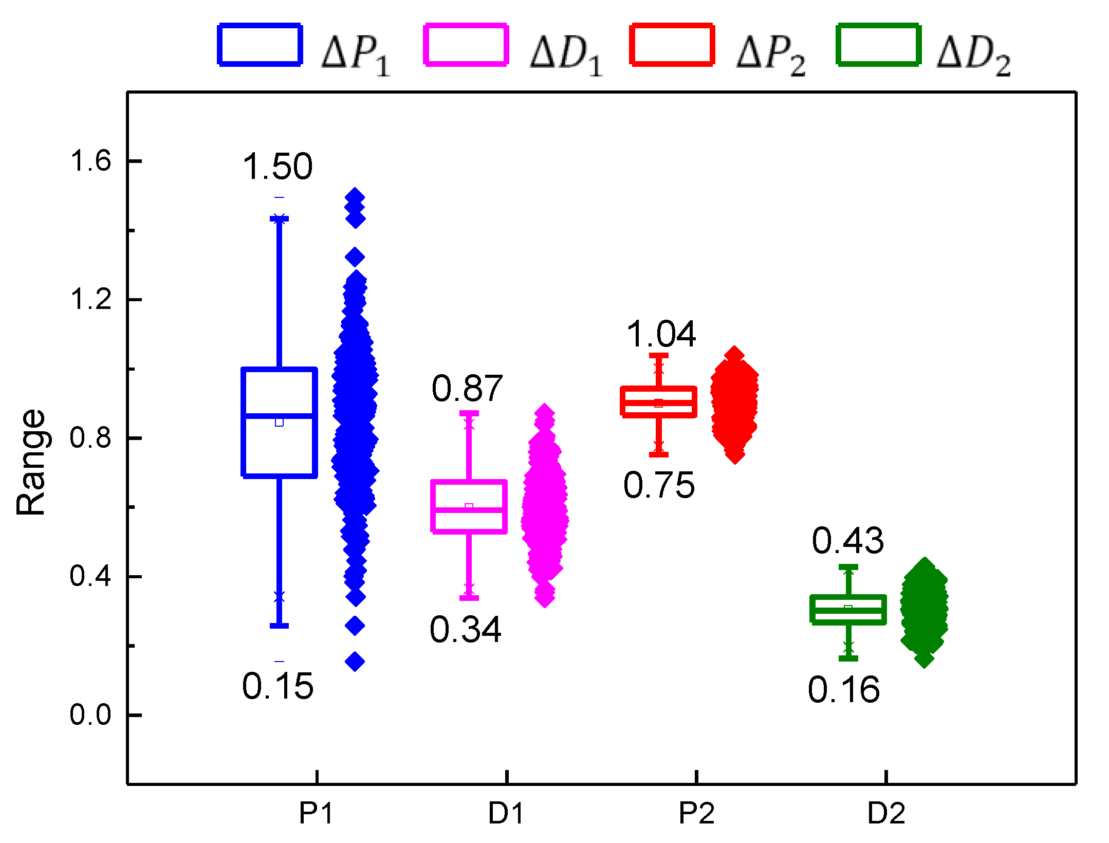
| Mean | Standard Deviation | Sum | Minimum | Median | Maximum | |
|---|---|---|---|---|---|---|
| 0.84623 | 0.21836 | 206.48024 | 0.15364 | 0.86328 | 1.49518 | |
| 0.59826 | 0.10214 | 145.97583 | 0.33797 | 0.59185 | 0.87246 | |
| 0.90078 | 0.05179 | 219.78983 | 0.75222 | 0.90156 | 1.0384 | |
| 0.30479 | 0.05151 | 74.36867 | 0.16412 | 0.30233 | 0.42815 |
| 50 km/h Driving Condition on the Road of Map-E | ||||
| Mean | Standard Deviation | Minimum | Maximum | |
| PID–RL Controller | 0.09325 | −0.32759 | ||
| ADRC-Controller | −0.06622 | 0.10941 | −0.37658 | 0.18714 |
| 60 km/h Driving Condition on Road of Map-E | ||||
| Mean | Standard Deviation | Minimum | Maximum | |
| PID–RL Controller | 0.10994 | −0.35013 | ||
| ADRC-Controller | −0.04492 | 0.10508 | −0.37490 | 0.27655 |
| Indicators | Mean | Standard Deviation | Minimum | Maximum | |
|---|---|---|---|---|---|
| PID Controller | Speed | 41.0455 | 8.4158 | 0 | 55 |
| Lateral error | −0.1030 | 0.3573 | −1.1125 | 0.9966 | |
| PID–RL Controller | Speed | 84.6887 | 16.9462 | 0 | 101 |
| Lateral error | −0.0137 | 0.1089 | −0.3844 | 0.6640 | |
| Human Driver | Speed | 51.5378 | 11.8857 | 0 | 71 |
| Lateral error | −0.0014 | 0.1135 | −0.6068 | 0.5521 |
| Mean | Standard Deviation | Minimum | Maximum | |
|---|---|---|---|---|
| Human−steer | −22.15445 | 69.05777 | −386 | 325 |
| PID−Steer | −42.81777 | 88.80323 | −447 | 536 |
| PID−RL−Steer | −22.06958 ↓ | 80.69866 ↓ | −390.8 ↓ | 403.2 ↓ |
| Mean | Standard Deviation | Minimum | Median | Maximum | |
|---|---|---|---|---|---|
| 53.84405 | 10.34426 | 16.2258 | 56.0301 | 79.3932 | |
| 92.10457 | 2.05332 | 85.6766 | 92.0764 | 98.2066 | |
| 39.07703 | 0.49852 | 37.5222 | 39.0849 | 40.747 | |
| 6.46417 | 0.24382 | 5.6081 | 6.46435 | 7.1453 |
Publisher’s Note: MDPI stays neutral with regard to jurisdictional claims in published maps and institutional affiliations. |
© 2021 by the authors. Licensee MDPI, Basel, Switzerland. This article is an open access article distributed under the terms and conditions of the Creative Commons Attribution (CC BY) license (https://creativecommons.org/licenses/by/4.0/).
Share and Cite
Ma, J.; Xie, H.; Song, K.; Liu, H. Self-Optimizing Path Tracking Controller for Intelligent Vehicles Based on Reinforcement Learning. Symmetry 2022, 14, 31. https://doi.org/10.3390/sym14010031
Ma J, Xie H, Song K, Liu H. Self-Optimizing Path Tracking Controller for Intelligent Vehicles Based on Reinforcement Learning. Symmetry. 2022; 14(1):31. https://doi.org/10.3390/sym14010031
Chicago/Turabian StyleMa, Jichang, Hui Xie, Kang Song, and Hao Liu. 2022. "Self-Optimizing Path Tracking Controller for Intelligent Vehicles Based on Reinforcement Learning" Symmetry 14, no. 1: 31. https://doi.org/10.3390/sym14010031
APA StyleMa, J., Xie, H., Song, K., & Liu, H. (2022). Self-Optimizing Path Tracking Controller for Intelligent Vehicles Based on Reinforcement Learning. Symmetry, 14(1), 31. https://doi.org/10.3390/sym14010031