A Continuous Terminal Sliding-Mode Observer-Based Anomaly Detection Approach for Industrial Communication Networks

Abstract

Dynamic traffic monitoring is a critical part of industrial communication network cybersecurity, which can be used to analyze traffic behavior and identify anomalies. In this paper, industrial networks are modeled by a dynamic fluid-flow model of TCP behavior. The model can be described as a class of systems with unmeasurable states. In the system, anomalies and normal variants are represented by the queuing dynamics of additional traffic flow (ATF) and can be considered as a disturbance. The novel contributions are described as follows: (1) a novel continuous terminal sliding-mode observer (TSMO) is proposed for such systems to estimate the disturbance for traffic monitoring; (2) in TSMO, a novel output injection strategy is proposed using the finite-time stability theory to speed up convergence of the internal dynamics; and (3) a full-order sliding-mode-based mechanism is developed to generate a smooth output injection signal for real-time estimations, which is directly used for anomaly detection. To verify the effectiveness of the proposed approach, the real traffic profiles from the Center for Applied Internet Data Analysis (CAIDA) DDoS attack datasets are used.

1. Introduction

An industrial network is a communication network that applied in an industrial environment, i.e., manufacturing, power generation, energy distribution, and transportation, with protocols to provide real-time control and monitoring of industrial systems. Due to the development of the Industrial Internet of Things (IIoT), a variety of technologies, such as sensors, wireless communications, and computing, have paved the way from local to remote networks for performing remote operations, monitoring, and maintenance through the Internet. Security concerns about the IIoT have been raised. On 21 October 2016, attackers utilize the Mirai IoT botnet to launch high-impact distributed denial of service (DDoS) attacks against the Dyn DNS service, which caused an extended Internet outage [1]. Therefore, the vulnerability of industrial networks have reinforced the importance of safety and security to protect industrial systems against cyber threats [2]. To detect and prevent the attacks, researchers are focused on designing traffic monitoring devices, such as firewalls and intrusion detection systems (IDSs), placed at different levels of industrial networks to detect and prevent attacks [3].

In the past years, many IDS methods have been proposed for monitoring malicious activities in industrial networks. By the types of information source, IDSs can be classified into two types: host-based IDSs (HIDSs) and network-based IDSs (NIDSs). HIDSs monitor the characteristics of information in hosts to detect anomalous behavior. A data stream mining-based HIDS is proposed for the advanced metering infrastructure to collect and analyze energy usage data [4]. A novel multiattribute HIDS is developed in supervisory control and data acquisition (SCADA) cybersystems [5]. On the other hand, NIDSs analyze network activities in terms of traffic volume, protocol usage, IP address, and so on. Several NIDSs are proposed at network gateways, e.g., firewalls or routers, to online monitor the whole networks. For example, a deep packet inspection method is proposed to deal with high-layer protocols in terms of performance indexes at firewalls [6]. However, the typical case of limited-size data packets are not considered. A Markov chain NIDS is investigated to study the performance of rule-based IP traffic include throughput, packet loss, and packet delay at firewalls [7]. Furthermore, a filtering system-based NIDS is developed to block spurious traffic by using an IP packet queuing engine [8]. With the increased complexity and the growing amount network usages, the static analytical approach fails to meet the monitoring criteria in accuracy and efficiency. Thus, the real-time monitoring approach is needed to analyze network traffic at network gateways to detect malicious attacks. The dynamics of industrial TCP networks in routers can be expressed as a fluid-flow model by using stochastic differential nonlinear equations [9]. Based on the model, some observers have been proposed for the dynamical network monitoring system [10]. The observers are capable to detect anomalies. Since the anomalies are being considered as perturbations in the systems, observers can be designed to estimate the anomalies [11].

The current observers for traffic monitoring can be classified into two categories: linear observers and nonlinear observers. The linear observer strategy is developed to feed back the output errors in a linear manner. For example, the Luenberger observers (LOs) are developed to monitor the TCP traffic flows [12]. Moreover, LOs are synthesized to reconstruct the unmeasurable congestion window, i.e., $C_{wnd}$, for traffic estimations. The time-delay observers are applied to supervise the network via TCP flow estimations and detecting anomalies. However, they are unable to accurately estimate the system states in the presence of unknown signals or uncertainties [13]. Thus, the fuzzy observers (FOs) are designed by using a Takagi-Sugeno (T-S) system that consists of a number of linear time-invariant models to achieve global performance [14], whereas the local linear observers of FOs are still hardly able to force the estimation errors to zero. The nonlinear observers, such as sliding-mode observers (SMOs), are applied for traffic monitoring [15,16]. SMOs are designed using sliding-mode control (SMC) method. SMC has unique properties, such as low sensitivity to parameter variations and strong robustness to external disturbances, and has been applied in many areas [17,18,19,20]. The existing SMOs can be classified into two types, i.e., linear SMOs and terminal SMOs. The linear SMOs that include conventional SMOs (CSMOs) and super-twisting observers (STOs) use the linear hypersurface with asymptotic stability. For example, CSMOs are proposed for traffic monitoring and detecting anomalies [21]. In the CSMOs, low-pass filters are used to soften the signals with high frequency components, which cause a phase lag and delay. To deal with the chattering phenomenon, STOs are proposed to estimate ATF without any low-pass filters [22]. However, the STOs are activated when the estimate errors converged to zero, which results in a long start-up time. In contrast, terminal SMOs employ the nonlinear a hypersurface and drive the estimate errors to the hypersurface in finit-time [23,24,25,26,27].

Different from the existing observer methods for anomaly detection under the network communication scenario [28,29,30], the novel terminal sliding-mode observer (TSMO) is proposed with the contributions described as: (1) TSMO is designed for disturbance estimation with the properties of finite-time convergence of the estimation error; (2) the proposed TSMO can increase the convergence speed of the internal dynamics to meet the criteria for real-time anomaly detection; (3) a full order sliding mode is designed to achieve a smooth output injection and is directly applied for estimation; and (4) the TSMO is proposed to increase the estimation dynamics of the abnormal traffic, in which the estimation error will converge to a bounded small area within a finite-time and then converge to zero asymptotically. For the network communication scenarios, it is required to meet two criterias: robustness and smooth output injection signals. The results of the estimation for ATF can be further used for the anomaly detection. The paper aims at overcoming the following three challenges from the theoretical viewpoints:

• How to develop an observer for a class of systems where parts of states are unmeasurable.
• How to increase the convergence speed of the internal dynamics in the observer.
• How to design a smooth output injection of the observer and apply it directly for the estimation algorithm.

The remainder of the paper is organized as follows. The fluid-flow model of industrial networks is described in Section 3. The sliding-mode observer for the system is proposed in Section 4. In Section 5, the practical traffic replay is carried out to illustrate the effectiveness of the proposed method. Finally, conclusions are given in Section 6.

2. Problem Formulation and Preliminaries

Consider a class of linear time-varying delay systems represented by

$$\dot{\mathit{x}}\left(t\right)=\mathit{A}\mathit{x}\left(t\right)+{\mathit{A}}_d\mathit{x}(t-\tau )+\mathit{b}u\left(t\right)+\mathit{d}\delta \left(t\right),$$

(1)

where $\mathit{x}\left(t\right)={\left[x_1\left(t\right),x_2\left(t\right)\right]}^T\in {\mathbb{R}}^2$ is the system state, $u\left(t\right)\in \mathbb{R}$ is the control input, $\tau =\tau \left(t\right)\in \mathbb{R}$ is the time delay, $\delta \left(t\right)\in \mathbb{R}$ is the disturbance, and $\mathit{A}=\left[a_{11},a_{12};a_{21},a_{22}\right]$, ${\mathit{A}}_d=\left[a_{11d},a_{12d};a_{21d},a_{22d}\right]$, $\mathit{b}={\left[1,0\right]}^T$, and $\mathit{d}={\left[0,1\right]}^T$ are time invariant system parameters.

Some assumptions are made as: (1). the system (1) is stable; (2). the state $x_2$ is measurable; and (3). the state $x_1$ is unmeasurable.

The objective in the paper is to design an observer for estimating the disturbance $\delta \left(t\right)$ in (1). Now, an observer is proposed for the system (1) in the form

$$\begin{array}{c}\hfill \dot{\hat{\mathit{x}}}\left(t\right)=\mathit{A}\hat{\mathit{x}}\left(t\right)+{\mathit{A}}_d\hat{\mathit{x}}(t-\tau )+\mathit{b}u\left(t\right)+\mathit{v}\left(t\right),\end{array}$$

(2)

where $\hat{\mathit{x}}\left(t\right)={\left[{\hat{x}}_1\left(t\right),{\hat{x}}_2\left(t\right)\right]}^T\in {\mathbb{R}}^2$ is the estimate of $\mathit{x}\left(t\right)$, and $\mathit{v}\left(t\right)={\left[v_1\left(t\right),v_2\left(t\right)\right]}^T\in {\mathbb{R}}^2$ is the output injection of the observer.

If the errors between the estimates and the true states are written as $\mathit{e}\left(t\right)=\hat{\mathit{x}}\left(t\right)-\mathit{x}\left(t\right)$, then, from (1) and (2), the following error system is obtained

$$\begin{array}{c}\hfill \dot{\mathit{e}}\left(t\right)=\mathit{A}\mathit{e}\left(t\right)+{\mathit{A}}_d\mathit{e}(t-\tau )-\mathit{d}\delta \left(t\right)+\mathit{v}\left(t\right),\end{array}$$

(3)

and the estimate of the disturbance $\delta \left(t\right)$ follows that

$$\begin{array}{c}\hfill \widehat{\delta }\left(t\right)=\underset{\mathit{e}\left(t\right)\to 0}{lim}{v}_2\left(t\right).\end{array}$$

(4)

The estimation process includes the following two steps:

• The error system (3) converges to zero asymptotically or in finite-time by using the output injection of the observer.
• Once the error system (3) converges to zero, the disturbance in (1) can be estimated using (4).

The output injection of the observer $\mathit{v}\left(t\right)$ in (2) can only utilize the measurable error $e_2$, i.e., $v_1=v_1\left(e_2\right)$, $v_2=v_2\left(e_2\right)$. The output injection $v_2=v_2\left(e_2\right)$ can be designed to force $e_2$ converging to zero, although there exists unmeasurable $e_1$ and disturbance $\delta \left(t\right)$ in the error system (3). However, in the conventional observer [22], there is no output injection $v_1$ for the internal dynamics of error system (3). In such a case, the error state $e_1$ will converge to zero asymptotically due to the assumption 1. As a result, the convergence of $e_1$ cannot be affected by the signal $v_2$ and may be very slow. To address this problem in the conventional methods, an output injection signal $v_1$ is proposed to the error system (3), which aims at speeding up the convergence of the internal dynamics of the error system (3).

When the error system (3) converges to zero, the estimate of the disturbance can be obtained using (4). Hence, the output injection of the observer $v_2\left(t\right)$ is required to be smooth, which is a challenge to the design of the SMO.

Two Lemmas are stated below and will be used in the proof of the Theorems later.

Lemma 1

([31]). Given a nonlinear system $\dot{\mathit{x}}=\mathit{f}\left(\mathit{x}\right)$, where $\mathit{x}\in {\mathbb{R}}^n$, $\mathit{f}\left(0\right)=0$, and $\mathit{f}\left(·\right):{\mathbb{R}}^n\to {\mathbb{R}}^n$ is a continuous function. If there exists a continuous positive definite function $V\left(\mathit{x}\right)$ such that $\dot{V}\left(\mathit{x}\right)+c{V}^{\alpha }\left(\mathit{x}\right)\le 0$, where $c>0$ and $\alpha \in (0,1)$ are two constants. Then, $V\left(\mathit{x}\right)$, $\forall V\left({\mathit{x}}_0\right)\ne 0$, approaches to zero in a finite-time T, where $T\le {V^1}^{-\alpha }\left(\mathit{x}\left(0\right)\right)/\left(c(1-\alpha )\right)$.

To prove the Theorems in the paper, the stability of the following form of linear systems with time-varying delay is considered:

$$\begin{array}{c}\hfill \left\{\begin{array}{c}\dot{\mathit{x}}\left(t\right)=\mathit{A}\mathit{x}\left(t\right)+{\mathit{A}}_d\mathit{x}(t-\tau \left(t\right)),t>0,\hfill \\ \mathit{x}\left(t\right)=\mathit{\phi }\left(t\right),t\in [-{\tau }_2,0]\hfill \end{array},\right.\end{array}$$

(5)

where $\mathit{x}\left(t\right)\in {\mathbb{R}}^n$ is the state, $\mathit{A}$ and ${\mathit{A}}_d$ are constant matrices with appropriate dimensions, the time delay, $\tau \left(t\right)$, is a time-varying continuous function that satisfies ${\tau }_1<\tau \left(t\right)<{\tau }_2$ and $\dot{\tau }\left(t\right)\le \mu$, where ${\tau }_1$, ${\tau }_2$, and $\mu$ are all known positive constants, and the initial condition, $\phi \left(t\right)\in {\mathbb{R}}^n$, is a continuous function of $t\in [-{\tau }_2,0]$.

Lemma 2

([32]). The system (5) is asymptotically stable if there exist matrices $\mathit{P}>0$; ${\mathit{Q}}_i>0$, ${\mathit{Z}}_j>0$, for $i=1,2,3$, and $j=1,2$; ${\mathit{N}}_i$, ${\mathit{M}}_i$, and ${\mathit{S}}_i$, $i=1,2$ with appropriate dimensions such that the following LMI holds:

$$\begin{array}{c}\hfill \Phi ={\left[{\mathit{\varphi }}_{\iota \nu }\right]}_{8\times 8}<0,\end{array}$$

(6)

whereΦis the symmetric matrix, $\iota ,\nu =1,2,\cdots ,8$, ${\mathbf{\varphi }}_{11}=2\mathit{PA}+{\mathit{Q}}_1+{\mathit{Q}}_2+{\mathit{Q}}_3+2{\mathit{N}}_1$, ${\mathbf{\varphi }}_{12}={\mathit{PA}}_d+{\mathit{N}}_2-{\mathit{N}}_1+{\mathit{S}}_1-{\mathit{M}}_1$, ${\mathbf{\varphi }}_{13}={\mathit{M}}_1$, ${\mathbf{\varphi }}_{14}=-{\mathit{S}}_1$, ${\mathbf{\varphi }}_{15}={\tau }_2{\mathit{N}}_1$, ${\mathbf{\varphi }}_{16}={\tau }_{12}{\mathit{S}}_1$, ${\mathbf{\varphi }}_{17}={\tau }_{12}{\mathit{M}}_1$, ${\mathbf{\varphi }}_{18}={\mathit{A}}_{11}\upsilon$, ${\mathbf{\varphi }}_{22}=-(1-\mu ){\mathit{Q}}_3+2{\mathit{S}}_2-2{\mathit{N}}_2-2{\mathit{M}}_2$, ${\mathbf{\varphi }}_{23}={\mathit{M}}_2$, ${\mathbf{\varphi }}_{24}=-{\mathit{S}}_2$, ${\mathbf{\varphi }}_{25}={\tau }_2{\mathit{N}}_2$, ${\mathbf{\varphi }}_{26}={\tau }_{12}{\mathit{S}}_2$, ${\mathbf{\varphi }}_{27}={\tau }_{12}{\mathit{M}}_2$, ${\mathbf{\varphi }}_{28}={{\mathit{A}}_{11}}_d\upsilon$, ${\mathbf{\varphi }}_{33}=-{\mathit{Q}}_1$, ${\mathbf{\varphi }}_{44}=-{\mathit{Q}}_2$, ${\mathbf{\varphi }}_{55}=-{\tau }_2{\mathit{Z}}_1$, ${\mathbf{\varphi }}_{66}=-{\tau }_{12}({\mathit{Z}}_1+{\mathit{Z}}_2)$, ${\mathbf{\varphi }}_{77}=-{\tau }_{12}{\mathit{Z}}_2$, ${\mathbf{\varphi }}_{88}=-\upsilon$, ${\mathbf{\varphi }}_{\iota \nu }=0$, for $\nu >\iota$ and $\iota =3,4,\cdots ,7$, $\upsilon ={\tau }_2{\mathit{Z}}_1+{\tau }_{12}{\mathit{Z}}_2$, and ${\tau }_{12}={\tau }_2-{\tau }_1$.

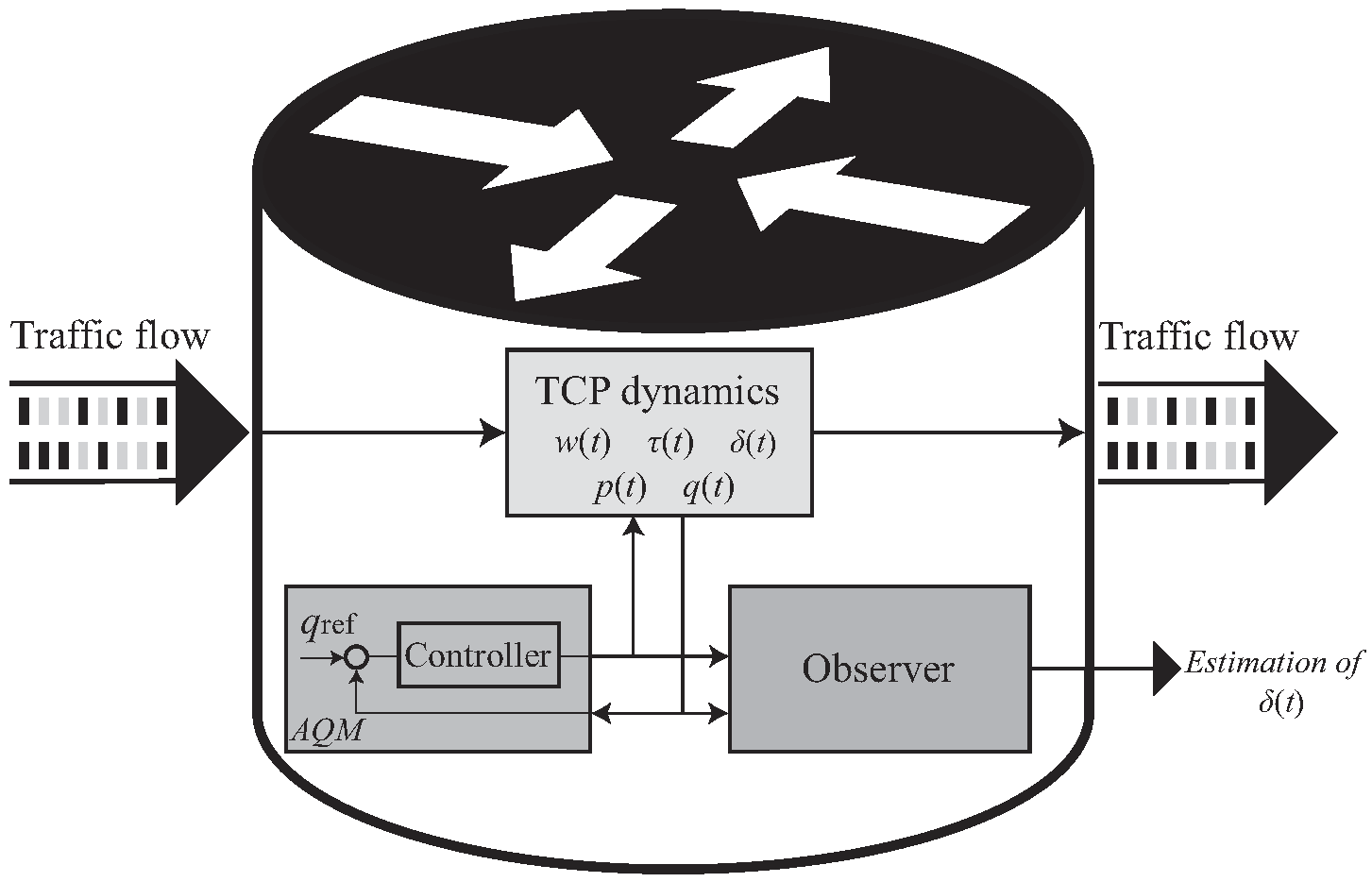
3. Fluid-Flow Model of Industrial Networks

Industrial networks interconnect various industrial control systems (ICS), e.g., local-area switched networks, such as distributed control systems, and wide-area routed networks, such as SCADA, to support the communication between devices. Most ICSs adopt some specialized protocols, such as Open Platform Communications, Modbus, Distributed Network Protocol, Inter-Control Center Protocol, Profibus, etc. However, these protocols were initially designed for serial communications and must been adapted to operate over TCP/IP networks, which is a standard Ethernet link layer and has been widely implemented at common network infrastructures. To this end, the industrial TCP/IP networks will be studied in the paper.

An industrial TCP/IP network consists of multiple hosts and clients in industrial control systems, which are physically connected in any number of topologies including star, tree, and even full-mesh. In industrial networks, a star topology is extremely common to connect to end devices [33]. So, a typical industrial TCP/IP network in a star topology is adopted in this study. In the topology, all nodes (hosts or any other industrial control systems peripherals) are connected to an industrial router. Each connected host has a dedicated, point-to-point connection between the host and the router. It is assumed that there are N homogeneous sources, i.e., all sources are the same in structure, nature, parameters, and software implementations. They connect to a destination (a host or a client devices) through a router, where two mechanisms are embedded: an Active Queue Management (AQM) and an observer. The AQM regulates the queue length in the router buffer with a randomization of choosing connections to notify the congestion, so that the network utilization can be improved. The observer is used to estimate the traffic flow and further detect its abnormal behavior of the traffics in industrial TCP/IP networks.

To describe the behavior of the traffics in industrial networks, the following fluid-flow model of TCP behavior can be used [9]:

$$\begin{array}{c}\hfill \left\{\begin{array}{cc}\hfill \dot{w}\left(t\right)=& \frac{1}{\tau \left(t\right)}-\frac{w\left(t\right)}{2}\frac{w(t-\tau (t\left)\right)}{\tau (t-\tau (t\left)\right)}p(t-\tau \left(t\right))\hfill \\ \hfill \dot{q}\left(t\right)=& N\frac{w\left(t\right)}{\tau \left(t\right)}-C+\delta \left(t\right)\hfill \\ \hfill \tau \left(t\right)=& \frac{q\left(t\right)}{C}+T_p\hfill \end{array},\right.\end{array}$$

(7)

where $w\left(t\right)$ is the average TCP congestion window size in packets. Congestion Window ($C_{wnd}$) is a TCP state variable that limits the amount of data the TCP can send into the network before receiving an ACK. $q\left(t\right)$ is expected queue length in packets. w and q are positive and bounded, i.e., $w\in \left[0,\overline{w}\right]$ and $q\in \left[0,\overline{q}\right]$, where $\overline{w}$ and $\overline{q}$ are known and denote maximum window size and buffer size, respectively. $\tau \left(t\right)$ is the round-trip time in seconds which induces time varying delay in the communication channel. $p\left(t\right)$ is the probability of packet loss and takes value at $\left[0,1\right]$. $T_p$ is the propagation delay in seconds. N and C are the numbers of TCP sections and the link bandwidth in packets/second, respectively.

In system (7), $\delta \left(t\right)$ represents the unmeasurable queuing dynamics of ATF in the network. It includes the modeling errors and anomalies. Both of them are uncertain and perturb the normal TCP/IP network behavior at the router level. In normal working conditions, $\delta \left(t\right)$ is around a fixed value, which forms a layer near the value; however, when an anomaly intrusion happens, it will suddenly increase.

The purpose of the paper is to estimate $\delta \left(t\right)$ only using $q\left(t\right)$ in (7). After obtaining the estimate of $\delta \left(t\right)$, we can detect and further analyze the anomalies.

The equilibrium point of system (7) is assumed as $(w_0,q_0)$, where $w_0$ is the equilibrium window size, and $q_0$ is the required queue length set by the AQM. $p_0$ is the equilibrium input value, and ${\tau }_0$ is the equilibrium round-trip time. They can be determined as follows by $\dot{w}\left(t\right)=0$ and $\dot{q}\left(t\right)=0$:

$$\begin{array}{c}\hfill \left\{\begin{array}{cc}\hfill {\tau }_0=& q_0/\phantom{q_{0}C}C+T_p\hfill \\ \hfill w_0=& {\tau }_{0}C/\phantom{{\tau }_{0}CN}N\hfill \\ \hfill p_0=& 2/\phantom{2{w_0}^2}{w}_0^2\hfill \end{array}.\right.\end{array}$$

The system (7) can be linearized around its equilibrium point. Defining the perturbation of the equilibrium point as $\Delta w\left(t\right)=w\left(t\right)-w_0$ and $\Delta q\left(t\right)=q\left(t\right)-q_0$, the dynamics of the industrial TCP networks (7) can be linearized to

$$\begin{array}{c}\hfill \left\{\begin{array}{cc}\hfill \Delta \dot{w}\left(t\right)=& -\frac{N}{{\tau }_0^{2}C}\left(\Delta w\left(t\right)+\Delta w(t-\tau (t\left)\right)\right)-\frac{1}{{\tau }_0^{2}C}(\Delta q\left(t\right)\hfill \\ \hfill & -\Delta q(t-\tau \left(t\right)))-\frac{{\tau }_0{C}^2}{2N^2}\Delta p(t-\tau \left(t\right))\hfill \\ \hfill \Delta \dot{q}\left(t\right)=& \frac{N}{{\tau }_0}\Delta w\left(t\right)-\frac{1}{{\tau }_0}\Delta q\left(t\right)+\delta \left(t\right)\hfill \end{array},\right.\end{array}$$

(8)

where $q\left(t\right)$ and $p\left(t\right)$ are available in the router. Some software programs, such as Netflow, PacketScope, and Loss Measurement Management, have been installed in routers. They can monitor and measure $p\left(t\right)$ [34]. The congestion window $w\left(t\right)$ cannot be used in the AQM or the observer because it is unmeasurable.

To simplify the design of the observer for the linearized model of the industrial TCP/IP network (8), a state transformation is made first.

Define a new state variable $x\left(t\right)=\Delta w\left(t\right)\in \mathbb{R}$, an output $y\left(t\right)=\Delta q\left(t\right)\in \mathbb{R}$, and a control $u\left(t\right)=\Delta p\left(t\right)\in \mathbb{R}$. Then, system (8) can be rewritten as

$$\begin{array}{c}\hfill \left\{\begin{array}{cc}\hfill \dot{x}\left(t\right)=& -a_{11}x\left(t\right)-a_{11}x(t-\tau \left(t\right))-a_{12}y\left(t\right)\hfill \\ \hfill & +a_{12}y(t-\tau \left(t\right))-b_{d}u(t-\tau \left(t\right))\hfill \\ \hfill \dot{y}\left(t\right)=& a_{21}x\left(t\right)-a_{22}y\left(t\right)+\delta \left(t\right)\hfill \end{array},\right.\end{array}$$

(9)

where $a_{11}=N/{{\tau }_0}^{2}C$, $a_{12}=1/{{\tau }_0}^{2}C$, $b_d={\tau }_0{C}^2/2N^2$, $a_{21}=N/{\tau }_0$, and $a_{22}=1/{\tau }_0$. C and N are defined in (7).

The time-delay $\tau \left(t\right)$ in (9) satisfies the following inequality:

$$\begin{array}{c}\hfill T_p\le \tau \left(t\right)\le \overline{q}/\phantom{\overline{q}C}C+T_p,\end{array}$$

(10)

where $\overline{q}$, C and $T_p$ are defined in (7).

It should be noted that the lower bound of $\tau \left(t\right)$ is $T_p$ as defined in (10). $T_p$ is the propagation delay at the circumstance of neither congestion nor queuing delay in a router. In addition, the upper bound of $\tau \left(t\right)$ in (10) is the combination of the propagation delay and the maximum queuing delay under the worst case of congestion in the router buffer, i.e., $\tau \left(t\right)$, cannot exceed $\overline{q}/C+T_p$.

The derivative of $\tau \left(t\right)$ can be assumed to satisfy

$$\begin{array}{c}\hfill \dot{\tau }\left(t\right)\le \mu ,\end{array}$$

(11)

where $\mu$ is a known positive constant.

The condition of (10) and (11) can be obtained as below. Differentiating the last equation in (7) with the time t gives

$$\begin{array}{c}\hfill \dot{\tau }\left(t\right)=\frac{1}{C}\left(\frac{Nw\left(t\right)+\delta \left(t\right)\tau \left(t\right)}{\tau \left(t\right)}-C\right).\end{array}$$

(12)

The term $Nw\left(t\right)+\delta \left(t\right)\tau \left(t\right)$ in (12) is actually the amount of data being transmitted in the TCP/IP network, which is physically constrained to the TCP/IP network capacities, namely $Nw\left(t\right)+\delta \left(t\right)\tau \left(t\right)\le BDP+\overline{q}$ where $\overline{q}$ is the buffer capacity defined in (7). BDP is the Bandwidth-Delay Product, which represents the amount of data that can be in transit [35]. BDP refers to the product of a data link’s capacity C and its round-trip delay time $\tau \left(t\right)$, i.e., $BDP=C\tau \left(t\right)$, where C and $\tau \left(t\right)$ are defined in (7). Normally, the buffer capacity of a router in (7) $\overline{q}$ is dependent on the BDP, i.e., $\overline{q}=\mu C\tau \left(t\right)$, where $\mu =1/\sqrt{N}$ is a constant [36]. Then, it can be obtained that $Nw\left(t\right)+\delta \left(t\right)\tau \left(t\right)\le C\tau \left(t\right)+\mu C\tau \left(t\right)$ and furthermore, we have the condition (11) is true.

The state variable $x\left(t\right)$ in the linearized model of the TCP/IP network (9) satisfies the inequality as follows:

$$\begin{array}{c}\hfill \left|x\left(t\right)\right|\le \overline{w},\end{array}$$

(13)

where $\overline{w}$ is the known positive constant, i.e., the maximum window size, and is defined in (7).

In TCP/IP networks, the window size refers to the amount of dada that a host is currently willing to send. Normally, the maximum window size $\overline{w}$ at a host is configured as a constant, i.e., $\overline{w}$ is set as $65,535$ (0xFFFF) bytes [37]. As seen as in (8) and (9), $x\left(t\right)$ is the perturbation around the equilibrium point of $w\left(t\right)$ that is limited to the known constant maximum window size $\overline{w}$. As $x\left(t\right)=\delta w\left(t\right)$, so $\left|x\right(t\left)\right|$ cannot exceed the maximum value of $w\left(t\right)$, i.e., the inequality (13) is true.

The aformentioned amount of data being transmitted in the TCP/IP network, $Nw\left(t\right)+\delta \left(t\right)\tau \left(t\right)$, in (12) includes traffic flow of all N TCP sections $Nw\left(t\right)$, as well as the dynamics of ATF$\delta \left(t\right)\tau \left(t\right)$. It is physically constrained to the TCP/IP network capacities, namely $\frac{Nw\left(t\right)}{\tau \left(t\right)}+\delta \left(t\right)\le C+\mu C$, which means that $\left|\delta \left(t\right)\right|\le (1+\mu )C$ holds because of $w\left(t\right)>0$, $\tau \left(t\right)>0$, i.e., $\left|\delta \left(t\right)\right|\le d_m$, where $d_m\le (1+\mu )C$ is a known positive constant which can be determined in the experiments.

As $\delta \left(t\right)$ is physically limited to the router communication capacity, its change rate is always constrained to $\left|\dot{\delta }\left(t\right)\right|\le d_m/T$, where T is the sampling period and kept as a constant $1/C$ [9]. Hence, we have $\left|\dot{\delta }\left(t\right)\right|\le d_m/T\le (1+\mu )C^2$, i.e., $\left|\dot{\delta }\left(t\right)\right|\le d_1$, where $d_1\le (1+\mu )C^2$ is a known positive constant. Summarizing the analysis above gives

$$\begin{array}{c}\hfill \left|\delta \left(t\right)\right|\le d_m,\left|\dot{\delta }\left(t\right)\right|\le d_1,\end{array}$$

(14)

where both $d_m$ and $d_1$ are known positive constants.

The block diagram of the AQM and observer in a router is shown in Figure 1. The AQM is utilized to control the queue length $q\left(t\right)$ to a required value by regulating the probability of packets loss $p\left(t\right)$. The inputs of the observer, i.e., $q\left(t\right)$ and $p\left(t\right)$, are measurable states. The outputs of the observer is the estimate of $\delta \left(t\right)$. The paper aims to design an observer for estimating the dynamics of ATF in real-time and further detecting anomalies in industrial networks.

Figure 1. Block diagram of the AQM and observer in an industrial switch/router.

4. Design of the TSM Observer

In the fluid-flow model of TCP/IP networks in (9), the ATF dynamics $\delta \left(t\right)$ can be considered as a disturbance. The estimate of $\delta \left(t\right)$ can be used for anomaly detection. To estimate $\delta \left(t\right)$, an observer is proposed as

$$\begin{array}{c}\hfill \left\{\begin{array}{cc}\hfill \dot{\hat{x}}\left(t\right)=& -a_{11}\hat{x}\left(t\right)-a_{11}\hat{x}(t-\tau \left(t\right))-a_{12}y\left(t\right)\hfill \\ \hfill & +a_{12}y(t-\tau \left(t\right))-b_{d}u(t-\tau \left(t\right))+v_1\left(t\right)\hfill \\ \hfill \dot{\widehat{y}}\left(t\right)=& a_{21}\hat{x}\left(t\right)-a_{22}y\left(t\right)+v_2\left(t\right)\hfill \end{array},\right.\end{array}$$

(15)

where $\hat{x}\left(t\right)$ and $\hat{y}\left(t\right)$ represent the estimates of the system state $x\left(t\right)$ and output $y\left(t\right)$, respectively, and $v_1\left(t\right)$ and $v_2\left(t\right)$ are output injection for the observer.

Define ${\xi }_1\left(t\right):=\hat{x}\left(t\right)-x\left(t\right)$ and ${\xi }_2\left(t\right):=\hat{y}\left(t\right)-y\left(t\right)$ as the errors between the system states and their estimates. The error system can be obtained from (9) and (15) as follows:

$$\begin{array}{c}\hfill \left\{\begin{array}{cc}\hfill {\dot{\xi }}_1\left(t\right)=& -a_{11}{\xi }_1\left(t\right)-a_{11}{\xi }_1(t-\tau \left(t\right))+v_1\left(t\right)\hfill \\ \hfill {\dot{\xi }}_2\left(t\right)=& a_{21}{\xi }_1\left(t\right)+v_2\left(t\right)-\delta \left(t\right)\hfill \end{array}.\right.\end{array}$$

(16)

It should be noted that the state ${\xi }_2$ in error system (16) is measurable and can be used in the design of the output injection. However, the state ${\xi }_1$ is unmeasurable and cannot be used in the design of the output injection, i.e., $v_1$ and $v_2$ in (16) can include only ${\xi }_2$.

4.1. Measurable Error Subsystem

The measurable error subsystem in (16) is firstly considered, namely

$$\begin{array}{c}\hfill {\dot{\xi }}_2\left(t\right)=a_{21}{\xi }_1\left(t\right)+v_2\left(t\right)-\delta \left(t\right).\end{array}$$

(17)

A TSM manifold is chosen as the following form [38,39]:

$$\begin{array}{c}\hfill s\left(t\right)={\dot{\xi }}_2\left(t\right)+\alpha {\xi }_2\left(t\right)+\beta {{\xi }_2}^{\varphi /\phantom{\varphi \rho }\rho }\left(t\right),\end{array}$$

(18)

where $\alpha ,\beta >0$ are constants, and $\rho$ and $\varphi$ are positive odd integers which satisfy $1<\rho /\varphi <2$.

Theorem 1.

The measurable error subsystem (17) will reach the ideal sliding manifold $s\left(t\right)=0$ firstly from any nonzero initial condition $s\left(0\right)\ne 0$ in a finite-time $t_r\le \left|s\left(0\right)\right|/{\eta }_2$, then converge to zero along $s\left(t\right)=0$ in another finite-time $t_s=\rho /\phantom{\rho \left(\alpha (\rho -\varphi )\right)}\left(\alpha (\rho -\varphi )\right)\left(ln(\alpha {\xi }_2^{(\rho -\varphi )/\phantom{(\rho -\varphi )\rho }\rho }\left(t_r\right)+\beta )-ln\beta \right)$, if $s\left(t\right)$ is selected as (18), and the output injection is given by

$$\begin{array}{cc}\hfill v_2\left(t\right)=& v_{2eq}\left(t\right)+v_{2n}\left(t\right)\hfill \end{array}$$

(19)

$$\begin{array}{cc}\hfill v_{2eq}\left(t\right)=& -a_{21}\hat{x}\left(t\right)-\alpha {\xi }_2\left(t\right)-\beta {\xi }_2{\left(t\right)}^{\varphi /\phantom{\varphi \rho }\rho }\hfill \\ \hfill {\dot{v}}_{2n}\left(t\right)=& -a_{12}{a}_{21}y\left(t\right)+a_{12}{a}_{21}y(t-\tau \left(t\right))\hfill \end{array}$$

(20)

$$\begin{array}{cc}\hfill & -a_{21}{b}_{d}u(t-\tau \left(t\right))-k_2\mathrm{sgn}\left(s\left(t\right)\right),\hfill \end{array}$$

(21)

where $k_2=2a_{11}{a}_{21}\overline{w}+d_1+{\eta }_2$, ${\eta }_2>0$ is a constant, and $\overline{w}$ and $d_1$ are defined in (7) and (14), respectively.

Proof. 

From (17), the manifold (18) can be rewritten as

$$\begin{array}{c}\hfill s\left(t\right)=a_{21}{\xi }_1\left(t\right)+v_2\left(t\right)-\delta \left(t\right)+\alpha {\xi }_2\left(t\right)+\beta {{\xi }_2}^{\varphi /\phantom{\varphi \rho }\rho }\left(t\right).\end{array}$$

Substituting (19) and (20) into the above gives

$$\begin{array}{c}\hfill s\left(t\right)=-a_{21}x\left(t\right)+v_{2n}\left(t\right)-\delta \left(t\right).\end{array}$$

(22)

Differentiating $s\left(t\right)$ in (22) with respect to time t along the measurable error subsystem (17) yields

$$\begin{array}{c}\hfill \begin{array}{cc}\hfill \dot{s}\left(t\right)=& -a_{21}\dot{x}\left(t\right)+{\dot{v}}_{2n}\left(t\right)-\dot{\delta }\left(t\right)\hfill \\ \hfill =& -a_{21}(-a_{11}x\left(t\right)-a_{11}x(t-\tau \left(t\right))-a_{12}y\left(t\right)\hfill \\ \hfill & +a_{12}y(t-\tau \left(t\right))-b_{d}u(t-\tau \left(t\right)))+{\dot{v}}_{2n}\left(t\right)-\dot{\delta }\left(t\right).\hfill \end{array}\end{array}$$

Further substituting (21) into the above equation gives

$$\begin{array}{c}\hfill \begin{array}{cc}\hfill \dot{s}\left(t\right)=& -a_{21}(-a_{11}x\left(t\right)-a_{11}x(t-\tau \left(t\right)))-(2a_{11}{a}_{21}\overline{w}\hfill \\ \hfill & +d_1+{\eta }_2)\mathrm{sgn}\left(s\left(t\right)\right)-\dot{\delta }\left(t\right).\hfill \end{array}\end{array}$$

Introduce a candidate Lyapunov function given by $V_1\left(t\right)=0.5s^2\left(t\right)$. Taking the derivative of $V_1\left(t\right)$ along the trajectories of (16), and using the above expression, it follows that

$$\begin{array}{c}\hfill \begin{array}{cc}\hfill s\left(t\right)\dot{s}\left(t\right)=& -a_{21}(-a_{11}x\left(t\right)-a_{11}x(t-\tau \left(t\right)))s\left(t\right)\hfill \\ \hfill & -(2a_{11}{a}_{21}\overline{w}+d_1+{\eta }_2)\left|s\left(t\right)\right|-\dot{\delta }\left(t\right)s\left(t\right)\hfill \\ \hfill \le & a_{21}(a_{11}\left|x\left(t\right)\right|+a_{11}\left|x(t-\tau (t\left)\right)\right|-2a_{11}\overline{w})\left|s\left(t\right)\right|\hfill \\ \hfill & +(\left|\dot{\delta }\left(t\right)\right|-d_1)\left|s\left(t\right)\right|-{\eta }_2\left|s\left(t\right)\right|\hfill \end{array}.\end{array}$$

From the conditions (13), (14) and the above, we have

$$\begin{array}{c}\hfill {\dot{V}}_1\left(t\right)=s\left(t\right)\dot{s}\left(t\right)\le -{\eta }_2\sqrt{2}{V_1}^{1/\phantom{12}2}\left(t\right)<0,\mathrm{for}s\left(t\right)\ne 0;\end{array}$$

it can be seen that measurable error subsystem (17) will reach to $s\left(t\right)=0$ within the finite-time $t_r\le \left|s\left(0\right)\right|/{\eta }_2$; in other words, $s\left(t\right)=0$, $\forall t\ge t_r.$ Once the ideal sliding-mode $s\left(t\right)=0$ is established, the measurable error subsystem (17) will maintain on $s\left(t\right)=0$ thereafter and behaves in an identical fashion as ${\dot{\xi }}_2\left(t\right)=-\alpha {\xi }_2\left(t\right)-\beta {{\xi }_2}^{\varphi /\phantom{\varphi \rho }\rho }\left(t\right)$, which will converge to zero along $s\left(t\right)=0$ in the finite-time $t_s$. □

Theorem 1 yields a method of designing the output injection in (17) by only using the measurable ${\xi }_2\left(t\right)$, which forces ${\xi }_2\left(t\right)$ to converge to zero in a finite-time, although there exist unmeasurable ${\xi }_1\left(t\right)$ and unknown disturbance $\delta \left(t\right)$ in (17).

4.2. Unmeasurable Error Subsystem

For the unmeasurable error subsystem in (16), namely

$$\begin{array}{c}\hfill {\dot{\xi }}_1\left(t\right)=-a_{11}{\xi }_1\left(t\right)-a_{11}{\xi }_1(t-\tau \left(t\right))+v_1\left(t\right).\end{array}$$

(23)

Define an area $\Gamma$ for unmeasurable ${\xi }_1$ near zero as

$$\begin{array}{c}\hfill \Gamma =\left\{{\xi }_1:\left|{\xi }_1-a_{21}^{-1}\delta \right|\le \phi \right\},\end{array}$$

(24)

where $\phi$ is a positive constant and defined as $\phi =a_{21}^{-1}{d}_m+\epsilon$, $d_m$ is defined in (14), and $\epsilon$ is a positive constant, which can be chosen by $0<\epsilon <a_{21}^{-1}{d}_m/2$.

The purpose of introducing the area $\Gamma$ is to design a output injection strategy in the following Theorem for increasing the convergence speed of the error ${\xi }_1$, when it is outside $\Gamma$.

Theorem 2.

The unmeasurable error subsystem (23) will converge to zero asymptotically, if the output injection is given by

$$\begin{array}{cc}\hfill v_1\left(t\right)=& \left\{\begin{array}{c}0,\left|{\tilde{\xi }}_1\left(t\right)\right|\le \phi \hfill \\ -k_1\mathrm{sgn}\left({\tilde{\xi }}_1\left(t\right)\right),\left|{\tilde{\xi }}_1\left(t\right)\right|>\phi \hfill \end{array}\right.\hfill \end{array}$$

(25)

$$\begin{array}{cc}\hfill {\tilde{\xi }}_1\left(t\right)=& \hat{x}\left(t\right)-a_{21}^{-1}{v}_{2n}\left(t\right)\hfill \end{array}$$

(26)

where $k_1=a_{11}\overline{w}+{\eta }_1$, $\overline{w}$ is a constant defined in (7), and ${\eta }_1>0$ is a constant.

Proof. 

The error state space of ${\xi }_1$ can be divided into two different areas, ${\Gamma }_o$ and $\Gamma$, and defined, respectively, as ${\Gamma }_o=\left\{{\xi }_1:\left|{\xi }_1-a_{21}^{-1}\delta \right|>\phi \right\}$ and $\Gamma =\left\{{\xi }_1:\left|{\xi }_1-a_{21}^{-1}\delta \right|\le \phi \right\}$, where $\phi >0$ is defined in (24). So, two different cases, i.e., Case 1 and 2, are considered.

Case 1: the error state ${\xi }_1$ is in area ${\Gamma }_o$. The measurable error subsystem (17) will move toward the sliding manifold $s=0$ under the output injection (19)–(21). When the measurable error subsystem reaches and stays on the sliding manifold, $s\left(t\right)=0$, under the output injection in Theorem 1, it follows from (22) that

$$\begin{array}{c}\hfill s\left(t\right)=a_{21}{\xi }_1\left(t\right)-a_{21}\hat{x}\left(t\right)+v_{2n}\left(t\right)-\delta \left(t\right)=0.\end{array}$$

(27)

From the above equation and (26), it gives that

$$\begin{array}{c}\hfill {\tilde{\xi }}_1\left(t\right)={\xi }_1\left(t\right)-a_{21}^{-1}\delta \left(t\right).\end{array}$$

(28)

As ${\xi }_1$ is in area ${\Gamma }_o$, the inequality $\left|{\xi }_1-a_{21}^{-1}\delta \right|>\phi$ holds. According to (28) and the above inequality, we can have that $\left|{\tilde{\xi }}_1\left(t\right)\right|>\phi$. So, the output injection (25) can be rewritten as

$$\begin{array}{c}\hfill v_1\left(t\right)=-k_1\mathrm{sgn}\left({\tilde{\xi }}_1\left(t\right)\right).\end{array}$$

(29)

As we have that ${\tilde{\xi }}_1\left(t\right)={\xi }_1\left(t\right)-a_{21}^{-1}\delta \left(t\right)<-\phi <0$, where $\phi =a_{21}^{-1}{d}_m+\epsilon$ is defined in (24), and $d_m$ is defined in (14), further, we can obtain that ${\xi }_1\left(t\right)<-\phi +a_{21}^{-1}\delta \left(t\right)=-a_{21}^{-1}(d_m-\delta \left(t\right))-\epsilon <0$. For the case of ${\tilde{\xi }}_1\left(t\right)={\xi }_1\left(t\right)-a_{21}^{-1}\delta \left(t\right)>\phi >0$, similarly, we can have that ${\xi }_1\left(t\right)>a_{21}^{-1}(d_m+\delta \left(t\right))+\epsilon >0$. So, it can be concluded that

$$\begin{array}{c}\hfill \mathrm{sgn}\left({\tilde{\xi }}_1\left(t\right)\right)=\mathrm{sgn}\left({\xi }_1\left(t\right)\right).\end{array}$$

(30)

According to the above equation, the output injection (29) can be rewritten as

$$\begin{array}{c}\hfill v_1\left(t\right)=-k_1\mathrm{sgn}\left({\xi }_1\left(t\right)\right);\end{array}$$

(31)

further substituting (31) into (23), the unmeasurable error subsystem (23) can be reformed as

$$\begin{array}{c}\hfill {\dot{\xi }}_1\left(t\right)=-a_{11}{\xi }_1\left(t\right)-a_{11}{\xi }_1(t-\tau \left(t\right))-k_1\mathrm{sgn}\left({\xi }_1\left(t\right)\right).\end{array}$$

(32)

Consider a candidate Lyapunov function $V_2\left(t\right)=0.5{\xi }_1^2\left(t\right)$. Taking the time-derivative of $V_2\left(t\right)$ yields

$$\begin{array}{c}\hfill \begin{array}{cc}\hfill {\dot{V}}_2=& {\xi }_1\left(t\right){\dot{\xi }}_1\left(t\right)=-a_{11}{\xi }_1^2\left(t\right)-a_{11}{\xi }_1(t-\tau \left(t\right)){\xi }_1\left(t\right)\hfill \\ \hfill & -k_1\left|{\xi }_1\left(t\right)\right|\hfill \\ \hfill \le & -{\eta }_1\left|{\xi }_1\left(t\right)\right|<0,\mathrm{for}\left|{\xi }_1\left(t\right)\right|\ne 0,\hfill \end{array}\end{array}$$

which means that, in Case 1, the error state ${\xi }_1$ in area ${\Gamma }_o$ must converge into the area $\Gamma$ in a finite-time.

Case 2: ${\xi }_1$ is in area $\Gamma$. The inequality $\left|{\xi }_1-a_{21}^{-1}\delta \right|\le \phi$ holds. According to (28) and the above inequality, it can be obtained that $\left|{\tilde{\xi }}_1\left(t\right)\right|\le \phi$. Therefore, the output injection (25) becomes $v_1\left(t\right)=0$, and the system (23) is rewritten as

$$\begin{array}{c}\hfill {\dot{\xi }}_1\left(t\right)=-a_{11}{\xi }_1\left(t\right)-a_{11}{\xi }_1(t-\tau \left(t\right)).\end{array}$$

(33)

To prove the stability of the system (33), consider the Lyapunov function [32] as

$$\begin{array}{c}\hfill \begin{array}{cc}\hfill V_3=& g{\xi }_1^2\left(t\right)+h_1{\int }_{t-T_p}^t{\xi }_1^2\left(s\right)ds+h_2{\int }_{t-\left(\overline{q}/\phantom{\overline{q}C}C+T_p\right)}^t{\xi }_1^2\left(s\right)ds\hfill \\ \hfill & +h_3{\int }_{t-\tau \left(t\right)}^t{\xi }_1^2\left(s\right)ds+{\int }_{-\left(\overline{q}/\phantom{\overline{q}C}C+T_p\right)}^0{\int }_{t+\theta }^t{z}_1{{\dot{\xi }}_1}^2\left(s\right)d\theta \hfill \\ \hfill & +{\int }_{-\left(\overline{q}/\phantom{\overline{q}C}C+T_p\right)}^{-T_p}{\int }_{t+\theta }^t{z}_2{{\dot{\xi }}_1}^2\left(s\right)d\theta \hfill \end{array},\end{array}$$

where g, $h_i$, for $i=1,2,3$, and $z_j$, for $j=1,2$, are all positive constants to be determined.

Define $X={[{\xi }_1\left(t\right),{\xi }_1(t-\tau \left(t\right)),{\xi }_1(t-T_p),{\xi }_1(t-(\overline{q}/C+T_p))]}^T$, $A={[-a_{11},-a_{11},0,0]}^T$, and $\Phi ={\left[{\varphi }_{\iota \nu }\right]}_{4\times 4}$ is the symmetric matrix, where $\iota ,\nu =1,2,\cdots ,4$, ${\varphi }_{11}=-2g{a}_{11}+h_1+h_2+h_3+2n_1$, ${\varphi }_{12}=-2g{a}_{11}+n_2-n_1+s_1-m_1$, ${\varphi }_{13}=m_1$, ${\varphi }_{13}=-s_1$, ${\varphi }_{22}=-(1-\mu )h_3+2s_2-2n_2-2m_2$, ${\varphi }_{23}=m_2$, ${\varphi }_{24}=-s_2$, ${\varphi }_{33}=-q_1$, ${\varphi }_{34}=0$, ${\varphi }_{44}=-q_2$, $M={[m_1,m_2,0,0]}^T$, $N={[n_1,n_2,0,0]}^T$, $S={[s_1,s_2,0,0]}^T$, and $\gamma$ is a sufficient small positive value.

Differentiating $V_3\left(t\right)$ with respect to time t along the error subsystem (33) gives

$$\begin{array}{c}\hfill \begin{array}{cc}\hfill {\dot{V}}_3=& 2g{\xi }_1\left(t\right){\dot{\xi }}_1\left(t\right)+h_1\left({{\xi }_1}^2\left(t\right)-{{\xi }_1}^2(t-T_p)\right)+h_2({{\xi }_1}^2\left(t\right)\hfill \\ \hfill & -{{\xi }_1}^2\left(t-(\overline{q}/\phantom{\overline{q}C}C+T_p))\right)-(1-\dot{\tau }\left(t\right))h_3{{\xi }_1}^2(t-\tau \left(t\right)))\hfill \\ \hfill & +(\overline{q}/\phantom{\overline{q}C}C+T_p)z_1{{\dot{\xi }}_1}^2\left(t\right)+\frac{\overline{q}}{C}{z}_2{{\dot{\xi }}_1}^2\left(t\right)+h_3{{\xi }_1}^2\left(t\right)\hfill \\ \hfill & -z_1{\int }_{t-\left(\overline{q}/\phantom{\overline{q}C}C+T_p\right)}^t{{\dot{\xi }}_1}^2\left(s\right)ds-{\int }_{t-\left(\overline{q}/\phantom{\overline{q}C}C+T_p\right)}^{t-T_p}{z}_2{{\dot{\xi }}_1}^2\left(s\right)ds\hfill \end{array},\end{array}$$

$$\begin{array}{c}\hfill \begin{array}{cc}\hfill \le & X^T[\Phi +A\left((\overline{q}/\phantom{\overline{q}C}C+T_p)z_1+\frac{\overline{q}}{C}{z}_2\right)A^T+\frac{\overline{q}}{C}M{z_2}^{-1}{M}^T\hfill \\ \hfill & +(\overline{q}/\phantom{\overline{q}C}C+T_p)N{z_1}^{-1}{N}^T+\frac{\overline{q}}{C}S{(z_1+z_2)}^{-1}{S}^T]X\hfill \\ \hfill & -{\int }_{t-\left(\overline{q}/\phantom{\overline{q}C}C+T_p\right)}^{t-\tau \left(t\right)}{(z_1+z_2)}^{-1}[X^{T}S+{\dot{\xi }}_1\left(s\right)(z_1+z_2)]\hfill \\ \hfill & \times \left[S^{T}X+(z_1+z_2){\dot{\xi }}_1\left(s\right)\right]ds\hfill \\ \hfill & -{\int }_{t-\tau \left(t\right)}^t{z_1}^{-1}\left[X^{T}N+{\dot{\xi }}_1\left(s\right)z_1\right]\left[N^{T}X+z_1{\dot{\xi }}_1\left(s\right)\right]ds\hfill \\ \hfill & -{\int }_{t-\tau \left(t\right)}^{t-T_p}{z_2}^{-1}\left[{\mathrm{X}}^{T}M+{\dot{\xi }}_1\left(s\right)z_2\right]\left[M^{T}X+z_2{\dot{\xi }}_1\left(s\right)\right]ds\hfill \end{array}.\end{array}$$

From (6) in Lemma 2 and the above inequality, it can be obtained as

$$\begin{array}{c}\hfill {\dot{V}}_3<-\gamma {\left|{\xi }_1\left(t\right)\right|}^2<0,\end{array}$$

(34)

which ensures the asymptotic stability of the error system (33), i.e., ${\xi }_1\left(t\right)$, will converge to zero asymptotically.

The state space of ${\xi }_1$ can be divided into two different areas, ${\Gamma }_o$ and $\Gamma$. In Case 1, when the state ${\xi }_1$ is in ${\Gamma }_0$, the output injection strategies (25)–(26) drive the error system (32) converging to the area $\Gamma$ in a finite time. Once the state ${\xi }_1$ reached and entered the area $\Gamma$, namely Case 2 occurred, and the error system (33) will converge to zero asymptotically. That means the the unmeasurable error subsystem (23) will converge to zero asymptotically. □

Remark 1.

In practice, the output injection strategies (25)–(26) are implemented by ${\prod }_{-\sigma ,\sigma }\left(s\right)\times v_1$, where ${\prod }_{-\sigma ,\sigma }\left(s\right)$ is a boxcar function and expressed by

$$\begin{array}{c}\hfill {\prod }_{-\sigma ,\sigma }\left(s\right)=\left\{\begin{array}{ccc}\hfill 1,& \hfill & \hfill \left|s\right|\le \sigma \\ \hfill 0,& \hfill & \hfill \left|s\right|>\sigma \end{array},\right.\end{array}$$

where $\sigma >0$ is a constant.

The whole state space of ${\xi }_1$ and ${\xi }_2$ can be divided into two different areas, ${\Omega }_1$ and ${\Omega }_2$, defined as ${\Omega }_1=\left\{({\xi }_1,{\xi }_2):\left|s\right|>\sigma \right\}$ and ${\Omega }_2=\left\{({\xi }_1,{\xi }_2):\left|s\right|\le \sigma \right\}$.

When the system states ${\xi }_1,{\xi }_2$ are in ${\Omega }_1$, the boxcar function ${\prod }_{-\sigma ,\sigma }\left(s\right)=0$, and then $v_1\left(t\right)$ in (25) is equal to zero, which means that the measurable error subsystem (17) has not reached to the sliding manifold $s\left(t\right)=0$. In this case, the output injection (25) has not been applied in the unmeasurable error subsystem (23).

The measurable error subsystem (17) will move toward the sliding manifold $s=0$ under the output injection (19)–(21). Once it reaches to $s=0$, the system states ${\xi }_1,{\xi }_2$ enter into the area ${\Omega }_2=\left\{({\xi }_1,{\xi }_2):\left|s\right|\le \sigma \right\}$. σ is selected as a small constant for practical implementation.

The output injection strategies (19)–(21) in Theorem 1 drive the error subsystem (17) toward the sliding manifold $s=0$ and remain on the manifold thereafter, which guarantees the system states ${\xi }_1,{\xi }_2$ to converge into the area ${\Omega }_2$ in a finite-time. Then, the unmeasurable error system (23) will converge to zero asymptotically.

In ideal condition, $\sigma =0$, i.e., the ideal sliding-mode $s=0$ can be detected. However, in practical environments, detecting ideal $s=0$ is not possible. So, we can just only detect an area near zero, $\left|s\right|<\sigma$. In this case, substituting (19) and (20) into (18), we have $a_{21}{\xi }_1\left(t\right)-\delta \left(t\right)=a_{21}\hat{x}\left(t\right)-v_{2n}\left(t\right)+s\left(t\right)$, where $\left|s\left(t\right)\right|<\sigma$. Hence, it can be chosen σ as $\sigma =\kappa \left|a_{21}{\tilde{\xi }}_1\left(t\right)\right|$, where $\kappa =0.02-0.05$. It should be noted that σ can affect only the convergence speed in dynamical process but cannot affect the final observation.

Theorem 3.

If the two output injection signals in the error system (16) are designed using Theorems 1 and 2, respectively, the estimation errors $\underset{t\to (t_r+t_s)}{lim}{\xi }_2\left(t\right)=0$ and $\underset{t\to \infty }{lim}{\xi }_1\left(t\right)=0$. Then, the ATF dynamics $\delta \left(t\right)$ in (9) can be estimated by as

$$\begin{array}{c}\hfill \underset{t\to \infty }{lim}{v}_2\left(t\right)=\underset{t\to \infty }{lim}\delta \left(t\right),\end{array}$$

(35)

where $v_2\left(t\right)$ is designed in (19).

Proof. 

Based on Theorem 1, the measurable error subsystem (16) under the output injection (19) will reach to the sliding manifold $s\left(t\right)=0$ in the finite-time $t_r$ and maintain on $s\left(t\right)=0$ thereafter. The unmeasurable error subsystem (17) will converge to zero in the finite-time along $s\left(t\right)=0$. Then, it follows from (17) that

$$\begin{array}{c}\hfill {\dot{\xi }}_2\left(t\right)=a_{21}{\xi }_1\left(t\right)+v_2\left(t\right)-\delta \left(t\right)=0.\end{array}$$

(36)

From Theorem 2, the unmeasurable error state ${\xi }_1\left(t\right)$ under the output injection (25) will converge to zero asymptotically. From (36), the ATF dynamics $\delta \left(t\right)$ can be estimated directly by the smooth $v_2\left(t\right)$ in (19) when the unmeasurable error state ${\xi }_1\left(t\right)$ converges to zero asymptotically. This completes the proof. □

5. Real Traffic Replay Results

The real traffic replay results are given to varify the effectiveness of the proposed TSMO method in real-time.

5.1. Real Traffic Replay Setup

For experimental purposes, we used the real traffic dataset from CAIDA, which is governed by the Regents of the University of California and located at the University of California San Diego (UCSD) [40].

In the paper, the CAIDA “DDoS Attack 2007” dataset is used to test the proposed method. This dataset contains approximately one hour of anonymized traffic traces from a DDoS attack on 4 August 2007 ($20:50:08$ UTC to $21:56:16$ UTC). The DDoS attack attempts to disrupt access to the targeted server and all of the bandwidth of the network connecting the server to the Internet, by consuming computing resources on the server. The 1-h trace is split up into 5-min pcap files, where pcap is an application programming interface for capturing network traffic. The total uncompressed size of the dataset is 21 GB. The traces only include attack traffic to the victim and responses to the attack from the victim. The non-attack traffic in the traces has been removed as much as possible. Traces in this dataset are anonymized using CryptoPAn prefix-preserving anonymization using a single key. The payload has been removed from all packets. These traces can be read with any software that reads the format of packet capture (pcap), including the CoralReef Software Suite, Tcpdump, Wireshark, and many others. The details of traffic features are shown in Table 1. In this experiment, the real-time DDoS attack scenarios for the CAIDA datasets are considered. This collection groups the backscatter datasets, which were created from the massive amount of data continuously collected from the UCSD Network Telescope.

Table 1. Traffic features of Caida “DDoS Attack 2007” dataset [40].

Maximum capture length for interface	0:65,000
First timestamp:	1,186,260,576.487629
Last timestamp:	1,186,260,876.482457
Unknown encapsulation:	0
IPv4 bytes:	37,068,253
IPv4 pkts:	166,448
IPv4 traffic:	8079
Unique IPv4 addresses:	136
Unique IPv4 source addresses:	132
Unique IPv4 destination addresses:	136
Unique IPv4 TCP source ports:	4270
Unique IPv4 TCP destination ports:	3348
Unique IPv4 UDP source ports:	1
Unique IPv4 UDP destination ports:	1
Unique IPv4 ICMP type/codes:	2

To study the network traffic behavior, a network simulator is used to set up network environments. It is a discrete event-based network simulator for networking research, which contains the necessary features, e.g., a traffic trace generator, to replay the real traffic traces profiles.

A typical star topology of the TCP/IP network consisting of a number of hosts and clients with one network gateway is considered in the study. There are N source agents and destination agents being created to represent the hosts and clients in the network, respectively, where $N=60$. The ‘newreno tcp’ agents are used for the sources with ‘ftp’ connections to generate long-lived TCP flows to the destination clients. The maximum value of $C_{wnd}$ in each ‘tcp’ agent is set to be the same as $0.12$ Mb. The link capacity C of the network gateway router is set to be 15 Mb. Moreover, the packet size is set to be 500 bytes. The connections between each host/client and the router are set by ‘full-duplex’, which construct bi-directional links at propagation delay $T_p=200$ ms. The proportional integral (PI) AQM mechanism is applied to regulate the queue length (QL) at a desired value of $q_0=175$ packets in router buffer [41]. The capacity of router buffer $\overline{q}$ is set to be 800 packets. A traffic trace generates payload bursts according to the given trace file of the DDoS attack profile from the CAIDA Dataset. In the network simulator, traffic trace is implemented by using the C++ class ‘TrafficTrace’, which is bound to the specified real DDoS attack traffic trace file in the OTcl domain.

A hundred distributed attackers are created and attached with the real traffic trace files from the CAIDA datasets. In the paper, an increasing rate attack profile of the CAIDA DDoS 2007 datasets is used to test the proposed method. This DoS attack lasts a period of five min.

The parameters in the linearized TCP/IP network model (9) are: $a_{11}=0.2630$, $a_{12}=0.0044$, $b_d=481.7708$, $a_{21}=243.2432$, and $a_{22}=4.0541$.

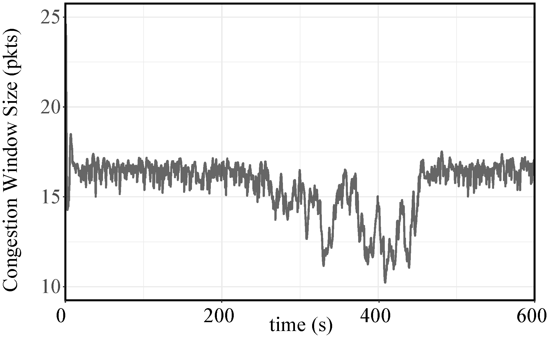
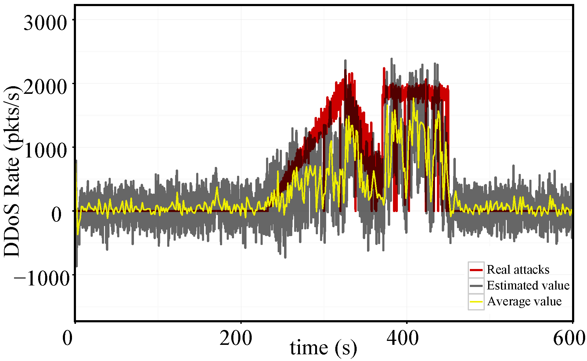
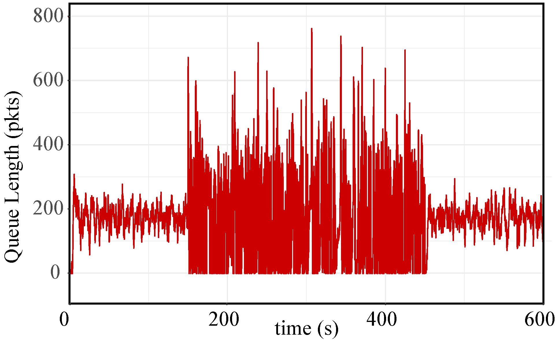
5.2. Real Traffic Replay Results and Discussion

Figure 2, Figure 3, Figure 4, Figure 5, Figure 6 and Figure 7 depict the experimental results of the proposed TSMO-based NTM in the scenarios of CAIDA Dataset-6 and Dataset-11. Figure 2 and Figure 5 shows the traffic dynamics of QL captured at the router, which includes the normal traffic flows and the DDoS attack profiles. With simple observations at this traffic dynamics of QL, the anomalies displayed in the traffic dynamics cannot be identified and detected in real-time. By contrast, the TSMO-based real-time NTM scheme, which is implemented at the router, is capable to extract TCP traffic flows from the total traffic dynamics in the buffer and estimate the dynamics of ATF for anomaly detection.

Figure 2. Queue length measured in router buffer in increasing rate attack profile of CAIDA Dataset-6.

Figure 3. Estimation of $C_{wnd}$ in increasing rate attack profile of CAIDA Dataset-6.

Figure 4. Estimation of attack rate in increasing rate attack profile of CAIDA Dataset-6.

Figure 5. Queue length measured in router buffer in increasing rate attack profile of CAIDA Dataset-11.

Figure 6. Estimation of $C_{wnd}$ in increasing rate attack profile of CAIDA Dataset-11.

Figure 7. Estimation of attack rate in increasing rate attack profile of CAIDA Dataset-11.

As the Theorem 1, the measurable error subsystem (17) will reach to the predesigned manifold (18), i.e., $s\left(t\right)=0$, within the finite-time $t_r$. Therefore the estimation error ${\xi }_2$ of QL is governed by the output injection (19) to converge to zero in the finite-time $t_s$ along $s\left(t\right)=0$.

In addition to forcing the estimation error ${\xi }_2$ to zero in the finite-time, the other aim is to speed up the convergence of the internal dynamics of the error system (16) for precision estimation to meet the real-time criteria. By Theorem 2, the internal dynamics, i.e., the estimation error ${\xi }_2$, is forced to the defined area (24) in the finite-time and then converges to zero asymptotically. As presented in Figure 3 and Figure 6, the congestion window is accurately estimated, which reflects the serious degradations in sending rate, throuput and bandwidth utilization in the networks when the DDoS attacks started in the scenario. From the Theorem 3, the dynamics of ATF, i.e., $\delta \left(t\right)$, which is represented by the increasing rate attack profile and the subgroup attack profile from the CAIDA datasets, is quickly and exactly estimated. The results of the estimated dynamics of DDoS rate are depicted in Figure 4 and Figure 7.

As the experimental results illustrated in Figure 2, Figure 3, Figure 4, Figure 5, Figure 6 and Figure 7, the proposed TSMO-based NTM presents a good tracking performances of the real traffic trace profile for anomaly detection with the main features of the SMC systems. This real traffic replay experimental results demonstrated the effectiveness and efficiency of the proposed TSMO algorithms in a real-time monitoring capability under real traffic profile environments.

5.3. Comparative Studies

Four different observer algorithms are evaluated in the real traffic replay tests.

5.3.1. The Luenberger Observer (LO)

The output injection strategies of the LO can be designed as [12]:

$$\begin{array}{c}\hfill \left\{\begin{array}{cc}\hfill v_1^{\mathrm{lo}}\left(t\right)& =-L_1^{\mathrm{lo}}(y\left(t\right)-{\widehat{y}}_{\mathrm{lo}}\left(t\right)),\hfill \\ \hfill v_2^{\mathrm{lo}}\left(t\right)& =-L_2^{\mathrm{lo}}(y\left(t\right)-{\widehat{y}}_{\mathrm{lo}}\left(t\right)),\hfill \end{array}\right.\end{array}$$

where ${\widehat{y}}_{\mathrm{lo}}\left(t\right)$ is the estimate of $y\left(t\right)$ in (9), $v_1^{\mathrm{lo}}\left(t\right)$ and $v_2^{\mathrm{lo}}\left(t\right)$ are the output injection signals of the observer, and $L_1^{\mathrm{lo}}$ and $L_2^{\mathrm{lo}}$ are the gains of the output injection.

5.3.2. The Conventional Sliding Mode Observer (CSMO)

The CSMO chooses the linear sliding surface by the following:

$s_{\mathrm{csmo}}\left(t\right)=c_{\mathrm{csmo}}{\xi }_2^{\mathrm{csmo}}\left(t\right)$, where $c_{\mathrm{csmo}}>0$ is a constant, and the estimation error ${\xi }_2^{\mathrm{csmo}}\left(t\right)$ is defined by ${\xi }_2^{\mathrm{csmo}}\left(t\right)={\widehat{y}}^{\mathrm{csmo}}\left(t\right)-y\left(t\right)$. The output injection $v_1^{\mathrm{csmo}}\left(t\right)$ is equal to zero, and the output injection $v_2^{\mathrm{csmo}}\left(t\right)$ is designed as [21]:

$$v_2^{csmo}\left(t\right)=L_{\mathrm{csmo}}{\xi }_2^{\mathrm{csmo}}\left(t\right)-k_{\mathrm{csmo}}\mathrm{sgn}\left(s_{\mathrm{csmo}}\left(t\right)\right),$$

with $L_{\mathrm{csmo}}<0$, $k_{\mathrm{csmo}}>0$ is the gain of the output injection.

As highly frequent switching phenomenon existed in $v_2^{csmo}\left(t\right)$ due to the signum function, a low-pass filter is needed to extract the equivalent signal.

5.3.3. The Super-Twisting Observer (STO)

A sliding-mode surface is selected as $s_{\mathrm{sto}}\left(t\right)={\xi }_2^{\mathrm{sto}}\left(t\right)$, where ${\xi }_2^{\mathrm{sto}}\left(t\right)={\widehat{y}}^{\mathrm{sto}}\left(t\right)-y\left(t\right)$. The $v_1^{\mathrm{sto}}\left(t\right)$ is equal to zero, and the $v_2^{\mathrm{sto}}\left(t\right)$ is designed by [22]:

$$\begin{array}{c}\hfill \left\{\begin{array}{cc}\hfill v_2^{\mathrm{sto}}\left(t\right)& =-k_1^{sto}{\left|s_{\mathrm{sto}}\left(t\right)\right|}^{0.5}\mathrm{sgn}\left(s_{\mathrm{sto}}\left(t\right)\right)+v_{2n}^{\mathrm{sto}}\left(t\right)\hfill \\ \hfill {\dot{v}}_{2n}^{\mathrm{sto}}\left(t\right)& =-k_2^{sto}\mathrm{sgn}\left(s_{\mathrm{sto}}\left(t\right)\right)\hfill \end{array},\right.\end{array}$$

where both $k_1^{sto}$ and $k_2^{sto}$ are positive constant.

5.3.4. The Terminal Sliding Mode Observer (TSMO)

The output injection strategies of the proposed TSMO are designed using Theorem 1 and 2.

Four observers are implemented as: (1). The parameters of the LO are designed as $L_1^{\mathrm{lo}}=5$ and $L_2^{\mathrm{lo}}=32$, and (2). for the CSMO, the parameters are designed as: $c_{\mathrm{csmo}}=20$, $L_{\mathrm{csmo}}=-100$, and $k_{\mathrm{csmo}}=1600$. (3). The parameters of the STO are chosen as $k_1^{\mathrm{sto}}=100$ and $k_2^{\mathrm{sto}}=1600$. (4). The proposed TSMO: $\alpha =15$, $\beta =5$, $\rho =5$, $\varphi =3$, $k_1=7.5$, and $k_2=1600$.

In order to make a fair comparison, the parameters of the four types of observer schemes are repeatedly tested, and, thereby, the optimal parameters are obtained. In the processing, the tradeoff between the dynamic performances and the steady-state performances of the closed-loop error system is made. In this condition, the convergence speed and steady-state performances are compared each other for these observers.

To make the quantitative comparisons among the four kinds of observer algorithms in terms of the steady-state performances of closed-loop error systems, Table 2 provides the average displacement error (ADE) and the standard deviation of displacement error (SDE) in the scenario. From the comparative results in Table 2, the proposed TSMO features the fastest dynamical response and the best steady-state accuracies of estimating $w\left(t\right)$ and $\delta \left(t\right)$ compared to other existing three observers.

Table 2. Comparisons of steady-state performances of four observers in scenario I.

Observers		LO	CSMO	STO	TSMO
$t_r$ ($\sec$)		/	$4.2$	$2.5$	$2.1$
$t_s$ ($\sec$)		/	Asymptoticaly	Asymptoticaly	$2.2$
${\xi }_1$ ($\mathrm{pkt}/\mathsf{s}$)	ADE	$1.97$	$1.97$	$1.97$	$0.73$
	SDE	$2.15$	$2.15$	$2.15$	$2.16$
${\xi }_2$ ($\mathrm{pkt}/\mathsf{s}$)	ADE	$6.36$	$35.36$	$3.26$	$0.50$
	SDE	$21.68$	$48.03$	$50.56$	$14.44$
$e_{ATF}$ ($\mathrm{pkt}/\mathsf{s}$)	ADE	$829.43$	$1092.28$	$562.18$	$267.51$
	SDE	$780.45$	$616.56$	$267.61$	$273.54$

6. Conclusions

This paper has proposed an SMO-based network traffic monitoring approach to estimate the ATF dynamics. The main contributions of this work can be summarized as follows: (i) One output injection of the observer is specially designed to be smooth using the full-order SMC technique. It can be directly used for the estimation of traffic flows in real time, does not need any low-pass filter. (ii) The novel strategy for another output injection of the observer is proposed to increase the convergence speed of the internal dynamics of the observer, which can improve the speed of the estimation algorithms. (iii) The proposed TSMO can be used for a class of linear systems with time-varying delay where some system states are unmeasurable. For the proposed observer, the parameters in the algorithms are to be carefully set. The experimental results have verified the efficiency of the proposed TSMO by comparative studies in real traffic profiles from the CAIDA DDoS attack datasets. The future work will focus on anomaly detection applications considering the multiple area communication networks.

References

- Yan, Q.; Huang, W.; Luo, X.; Gong, Q.; Yu, F.R. A multi-level DDoS mitigation framework for the industrial internet of things. IEEE Commun. Mag. 2018, 56, 30–36. [Google Scholar] [CrossRef]
- Sarker, I.H.; Abushark, Y.B.; Alsolami, F.; Khan, A.I. Intrudtree: A machine learning based cyber security intrusion detection model. Symmetry 2020, 12, 754. [Google Scholar] [CrossRef]
- Zegzhda, D.; Lavrova, D.; Pavlenko, E.; Shtyrkina, A. Cyber attack prevention based on evolutionary cybernetics approach. Symmetry 2020, 12, 1931. [Google Scholar] [CrossRef]
- Faisal, M.A.; Aung, Z.; Williams, J.R.; Sanchez, A. Data-stream-based intrusion detection system for advanced metering infrastructure in smart grid: A feasibility study. IEEE Syst. J. 2015, 9, 31–44. [Google Scholar] [CrossRef]
- Yang, Y.; McLaughlin, K.; Sezer, S.; Littler, T.; Im, E.G. Multiattribute SCADA-specific intrusion detection system for power networks. IEEE Trans. Power Del. 2014, 29, 1092–1102. [Google Scholar] [CrossRef] [Green Version]
- Skybakmoen, T. Next Generation Firewall Comparative Analysis- Security; NSS Labs: Austin, TX, USA, 2014; pp. 1–20. [Google Scholar]
- Niu, Y.; Ho, D.W.C. Design of sliding mode control subject to packet losses. IEEE Trans. Autom. Control 2010, 55, 2623–2628. [Google Scholar] [CrossRef]
- Zhang, S.S.; Shang, W.L.; Wan, M.; Zhang, H.; Zeng, P. Security defense module of Modbus TCP communication based on region/enclave rules. Comput. Eng. Des. 2014, 35, 3701–3707. [Google Scholar]
- Misra, V.; Gong, W.; Towsley, D. Fluid-based analysis of a network of AQM routers supporting TCP flows with an application to RED. Comput. Commun. Rev. 2000, 30, 151–160. [Google Scholar] [CrossRef]
- Ariba, Y.; Gouaisbaut, F.; Labit, Y. Feedback control for router management and TCP/IP network stability. IEEE Trans. Netw. Service Manag. 2009, 6, 255–266. [Google Scholar] [CrossRef]
- Hollot, C.V.; Misra, V.; Towsley, D.; Gong, W. Analysis and design of controllers for AQM routers supporting TCP flows. IEEE Trans. Autom. Control 2002, 47, 945–959. [Google Scholar] [CrossRef] [Green Version]
- Ariba, Y.; Gouaisbaut, F.; Rahme, S.; Labit, Y. Traffic monitoring in transmission control protocol/active queue management networks through a time-delay observer. IET Control Theory Appl. 2012, 6, 506–517. [Google Scholar] [CrossRef]
- Cao, L.; Li, H.; Wang, N.; Zhou, Q. Observer-based event-triggered adaptive decentralized fuzzy control for nonlinear large-scale systems. IEEE Trans. Fuzzy Syst. 2018, 27, 1201–1214. [Google Scholar] [CrossRef]
- Wang, Y.; Xie, X.; Chadli, M.; Xie, S.; Peng, Y. Sliding mode control of fuzzy singularly perturbed descriptor systems. IEEE Trans. Fuzzy Syst. 2020. early access. [Google Scholar] [CrossRef]
- Hou, H.; Yu, X.; Xu, L.; Restam, K.; Cao, Z. Finite-time continuous terminal sliding mode control of servo motor systems. IEEE Trans. Ind. Electron. 2020, 67, 5647–5656. [Google Scholar] [CrossRef]
- Hou, H.; Yu, X.; Fu, Z. Sliding-mode control of uncertain time-varying systems with state delays: A non-negative constraints approach. IEEE Trans. Syst. Man, Cybern. Syst. 2020. early access. [Google Scholar] [CrossRef]
- Xu, W.; Qu, S.; Zhao, L.; Zhang, H. An Improved Adaptive Sliding Mode Observer for Middle- and High-Speed Rotor Tracking. IEEE Trans. Power Electron. 2021, 36, 1043–1053. [Google Scholar] [CrossRef]
- Gong, C.; Hu, Y.; Gao, J.; Wang, Y.; Yan, L. An improved delay-suppressed sliding-mode observer for sensorless vector-controlled PMSM. IEEE Trans. Ind. Electron. 2021, 67, 5913–5923. [Google Scholar] [CrossRef]
- Li, H.; Shi, P.; Yao, D. Adaptive Sliding-Mode Control of Markov Jump Nonlinear Systems with Actuator Faults. IEEE Trans. Autom. Control 2017, 62, 1933–1939. [Google Scholar] [CrossRef]
- Wang, Y.; Gao, Y.; Karimi, H.R.; Shen, H.; Fang, Z. Sliding Mode Control of Fuzzy Singularly Perturbed Systems With Application to Electric Circuit. IEEE Trans. Syst. Man, Cybern. Syst. 2018, 48, 1667–1675. [Google Scholar] [CrossRef]
- Rahme, S.; Labit, Y.; Gouaisbaut, F. Sliding mode observer for anomaly detection in TCP/AQM networks. In Proceedings of the IEEE Second International Conference on Communication Theory, Reliability, and Quality of Service (CTRQ’2009), Colmar, France, 20–25 July 2009; pp. 113–118. [Google Scholar]
- Rahme, S.; Labit, Y.; Gouaisbaut, F.; Floquet, T. Sliding modes for anomaly observation in TCP networks: From theory to practice. IEEE Trans. Control Syst. Technol. 2013, 21, 1031–1038. [Google Scholar] [CrossRef] [Green Version]
- Hou, H.; Yu, X.; Xu, L.; Chuei, R.; Cao, Z. Discrete-time terminal sliding-mode tracking control with alleviated chattering. IEEE ASME Trans. Mechatron 2019, 24, 1808–1817. [Google Scholar] [CrossRef]
- Hou, H.; Yu, X.; Fu, Z. Sliding mode control of networked control systems: An auxiliary matrices-based approach. IEEE Trans. Autom. Control 2021. early access. [Google Scholar] [CrossRef]
- Yang, H.; Yin, S. Reduced-Order Sliding-Mode-Observer-Based Fault Estimation for Markov Jump Systems. IEEE Trans. Autom. Control 2019, 64, 4733–4740. [Google Scholar] [CrossRef]
- Chen, S.; Zhang, X.; Wu, X.; Tan, G.; Chen, X. Sensorless Control for IPMSM Based on Adaptive Super-Twisting Sliding-Mode Observer and Improved Phase-Locked Loop. Energies 2019, 12, 1225. [Google Scholar] [CrossRef] [Green Version]
- Zheng, W.; Xia, B.; Wang, W.; Lai, Y.; Wang, M.; Wang, H. State of Charge Estimation for Power Lithium-Ion Battery Using a Fuzzy Logic Sliding Mode Observer. Energies 2019, 12, 2491. [Google Scholar] [CrossRef] [Green Version]
- Khalil, H.K.; Praly, L. High-gain observers in nonlinear feedback control. Int. J. Robust. Nonlinear Control. 2014, 24, 993–1015. [Google Scholar] [CrossRef]
- Beltran-Carbajal, F.; Valderrabano-Gonzalez, A.; Favela-Contreras, A.R.; Rosas-Caro, J.C. Active disturbance rejection control of a magnetic suspension system. Asian J. Control 2015, 17, 842–854. [Google Scholar] [CrossRef]
- Kim, K.S.; Rew, K.H.; Kim, S. Disturbance observer for estimating higher order disturbances in time series expansion. IEEE Trans. Autom. Control 2015, 17, 842–854. [Google Scholar]
- Bhat, S.P.; Bernstein, D.S. Finite-time stability of continuous autonomous systems. SIAM J. Control Optim. 2000, 38, 751–766. [Google Scholar] [CrossRef]
- He, Y.; Wang, Q.; Linb, C.; Wua, M. Delay-range-dependent stability for systems with time-varying delay. Automatica 2007, 43, 371–376. [Google Scholar] [CrossRef]
- Hatzivasilis, G.; Fysarakis, K.; Soultatos, O.; Askoxylakis, I.; Demetriou, G. The Industrial Internet of Things as an enabler for a Circular Economy Hy-LP: A novel IIoT protocol, evaluated on a wind park’s SDN/NFV-enabled 5G industrial network. Comput. Commun. 2018, 119, 127–137. [Google Scholar] [CrossRef]
- Chuck, F.; Moon, S.; Lyles, B.; Cotton, C.; Khan, M.; Moll, D.; Rockell, R.; Seely, T.; Diot, S.C. Packet level traffic measurements from the sprint IP backbone. IEEE Netw. 2003, 17, 6–16. [Google Scholar]
- Jacobson, V.; Braden, R.T. TCP extensions for long-delay paths. Network Working Group Request for Comments: 1072. 1988. Available online: https://www.rfc-editor.org/info/rfc1072 (accessed on 17 May 2020).
- Appenzeller, G.; Keslassy, I.; McKeown, N. Sizing router buffers. Comput. Commun. Rev. 2004, 34, 281–292. [Google Scholar] [CrossRef]
- Stevens, W. TCP slow start, congestion avoidance, fast retransmit, and fast recovery algorithms. Network Working Group Request for Comments: 2001. 1996. Available online: https://datatracker.ietf.org/doc/html/rfc2001 (accessed on 17 May 2020).
- Feng, Y.; Yu, X.; Man, Z. Non-singular terminal sliding mode control of rigid manipulators. Automatica 2002, 38, 2159–2167. [Google Scholar] [CrossRef]
- Feng, Y.; Han, F.; Yu, X. Chattering free full-order sliding-mode control. Automatica 2014, 50, 1310–1314. [Google Scholar] [CrossRef]
- The CAIDA UCSD “DDoS Attack 2007” Dataset. Available online: https://www.caida.org/data/passive/ddos-20070804_dataset.xml (accessed on 17 May 2020).
- Hollot, C.V.; Misra, V.; Towsley, D.; Gong, W. On designing improved controllers for AQM routers supporting TCP flows. In Proceedings of the IEEE INFOCOM’ 2001, Anchorage, AK, USA, 24–26 April 2001; Volume 3, pp. 1726–1734. [Google Scholar]
Publisher’s Note: MDPI stays neutral with regard to jurisdictional claims in published maps and institutional affiliations. |
© 2022 by the authors. Licensee MDPI, Basel, Switzerland. This article is an open access article distributed under the terms and conditions of the Creative Commons Attribution (CC BY) license (https://creativecommons.org/licenses/by/4.0/).