On Enhanced GLM-Based Monitoring: An Application to Additive Manufacturing Process

Abstract

Innovations in technology assist the manufacturing processes in producing high-quality products and, hence, become a greater challenge for quality engineers. Control charts are frequently used to examine production operations and maintain product quality. The traditional charting structures rely on a response variable and do not incorporate any auxiliary data. To resolve this issue, one popular approach is to design charts based on a linear regression model, usually when the response variable shows a symmetric pattern (i.e., normality). The present work intends to propose new generalized linear model (GLM)-based homogeneously weighted moving average (HWMA) and double homogeneously weighted moving average (DHWMA) charting schemes to monitor count processes employing the deviance residuals (DRs) and standardized residuals (SRs) of the Poisson regression model. The symmetric limits of HWMA and DHWMA structures are derived, as SR and DR statistics showed a symmetric pattern. The performance of proposed and established methods (i.e., EWMA charts) is assessed by using run-length characteristics. The results revealed that SR-based schemes have relatively better performance as compared to DR-based schemes. In particular, the proposed SR-DHWMA chart outperforms the other two, namely SR-EWMA and SR-HWMA charts, in detecting shifts. To illustrate the practical features of the study’s proposal, a real application connected to the additive manufacturing process is offered.

1. Introduction

For the surveillance of a process, the samples from a manufacturing line are taken and examined to guarantee that the product’s standard is satisfactory. Commonly, the variations in the quality aspects of any process are of two types. One is assignable cause variation, which can be detected and eliminated. Another is common cause variation, which is the inherent part of a manufacturing process and cannot be removed [1,2]. Control charts are conventional real-time statistical process control (SPC) tools utilized to differentiate such variations in the quality characteristics of a process. One simple control chart incorporates two horizontal lines showing the lower and upper control limits (i.e., LCL and UCL). If the plotted sample points are between the two limits, the process is deemed to be in control (IC), while if they are beyond the limits, the process is regarded as being out of control (OOC) [2,3]. Some production processes generate count data or the data which take only discrete and non-negative integers. The most common method to model the count data is the Poisson distribution [4], which can be employed to find how often the independent events are likely to happen within a specific time frame.

In the literature, many procedures have been recommended to examine Poisson distributed counts. The classical c and u control charts are the most commonly used techniques to surveil the Poisson distributed process [5]. For the count of nonconformities, Khoo [6] discussed the Poisson moving average (MA) control chart and found a new approach better than the c chart. Several researchers introduced different versions of the Poisson Exponentially Weighted Moving Average (EWMA) control chart (i.e., PEWMA chart) and revealed that the PEWMA chart’s ARL capabilities were more satisfactory than the Shewhart c chart’s [7,8,9]. The PEWMA chart’s idea is further extended to the Poisson double EWMA (PDEWMA) structure by Zhang et al. [10]. Shu et al. [11] originated the one-sided Poisson EWMA chart that spots upward shifts in Poisson rates. Shewhart- and EWMA-based control charts were proposed by Yamauchi et al. [12] for examining the ratio of two Poisson rates. Weiß [13] presented a s-EWMA chart to observe the serially dependent Poisson counts. Zhou et al. [14] and Zhou et al. [15] discussed EWMA charts for Poisson procedures in relation to unequal sample sizes. Sheu et al. [16] created generally weighted moving average (GWMA) charts to supervise Poisson observations. Chiu et al. [17] extended the Poisson GWMA chart to the Poisson double GWMA chart with rapid initial response properties. An EWMA control chart formed on ranked set-sampling techniques to observe Poisson processes were discussed by Abujiya et al. [18]. Lucas [19] and White et al. [20] suggested a Poisson cumulative sum (CUSUM) chart to spot small changes in the Poisson process mean level, and found it excellent relative to the c chart. Abujiya et al. [21] developed CUSUM control charts to evaluate the location parameter of a Poisson procedure exerting ranked set sampling. Jiang et al. [22] discussed a class of weighted CUSUM schemes for supervising Poisson processes in relation to unequal sample sizes. Moreover, for effective monitoring of non-confirming objects, Abbasi [23] proposed a Poisson progressive mean (PPM) control chart, which was further continued by Alevizakos et al. [4], utilizing the double progressive mean statistic. The literature on multivariate Poisson processes can be found in References [24,25,26,27].

There are some processes in which the quality is explained by a relationship between the variable of interest and a covariate known as a profile. The Poisson regression model is utilized to fit the data with covariates when the variable of interest follows the Poisson distribution. In this favor, Amiri et al. [28] evaluated the $T^2$ based methods for supervising Poisson response profiles. The influence of parameterization on the surveillance of Poisson regression profiles was analyzed by Maleki et al. [29]. Kuo et al. [30] presented a chart for the multivariate Poisson process by using a multiple linear regression model. Poisson regression based EWMA control chart was studied by Wen et al. [31]. Some other GLM-based control charts are presented in References [32,33,34,35,36]. In the literature, most of the control charts are derived from the residuals calculated by GLM modeling. For instance, Park et al. [37] studied control chart systems formed on estimated randomized quantile residuals of a fitted regression model. Mammadova et al. [38] proposed the control charts that use ridge deviance residuals as a basis for assessing both Poisson and COM-Poisson profiles. Marcondes Filho et al. [39] and Park et al. [40] studied deviance residual control charts for supervising count data by incorporating GLM together with principal component analysis. Jamal et al. [41] designed EWMA and CUSUM structures formulated on deviance and randomized quantile residuals of the COM-Poisson regression model.

Skinner et al. [42] examined a semiconductor process using control charts comprising generalized linear models. They studied complex datasets through multiple inputs and outputs and showed that GLM-based control charts outperform multiple traditional c charts to detect changes in the mean of counts. Skinner et al. [43] suggested a control chart that depends on a generalized linear model known as R-chart to examine deviance residuals resulting from a Poisson regression model. Furthermore, a novel link function for the Poisson regression model is offered by Asgari et al. [44]. They developed Shewhart and EWMA control charts to monitor standardized residuals of Poisson regression (that is, SR-Shewhart and SR-EWMA charts). They found the SR-EWMA chart to be superior to the SR-Shewhart chart.

Moreover, Asgari et al. [44] also extended the R-chart proposed by Skinner et al. [43] into the EWMA structure and called it the R-EWMA chart. The aforementioned GLM-based strategies have focused on Shewhart, EWMA and CUSUM structures. In order to improve the surveillance of the manufacturing process, we designed new homogeneously weighted moving average (HWMA) and double homogeneously weighted moving average (DHWMA) type control charts to monitor deviance and standardized residuals of the Poisson regression model (that is, R/SR-HWMA and R/SR-DHWMA charts). Many researchers have recently discovered that the HWMA structure has a superior detection ability to the EWMA chart [45,46,47,48,49,50,51]. Moreover, another advantage of R/SR-HWMA and R/SR-DHWMA charts is that they have symmetric limits, as deviance and standardized residuals show symmetric behavior. Furthermore, the proposed control charts’ ability is assessed by means of Run Length (RL) and compared with existing R-EWMA and SR-EWMA charts. In addition, the suggested procedures are applied to a real-life dataset that belongs to the 3D manufacturing process.

The remainder of the article is arranged as follows: The count model used in this study is described in Section 2. The formation of the suggested control charts that depend on Poisson model’s deviance residuals and standardized residuals is covered in Section 3. In Section 4, the performance evaluations of the proposed schemes based on a comprehensive simulation study are provided. Moreover, Section 5 comprises an application of proposed schemes to a real-life dataset that belongs to the 3D manufacturing process. Section 6 concludes with a summary, conclusion and recommendations for the future.

2. The Poisson Regression Model

The ordinary least square (OLS) technique is regarded as the root for control charts that are based on a model, but the use of OLS declines when the variable of interest is not normally distributed. The control charts that originated from the generalized linear model come in handy when the variable of interest is a part of the exponential family. Binomial, Gaussian, Gamma, Poisson, Inverse Gaussian and Exponential distributions are all part of the exponential family. If $Y$ is a random variable with a Poisson distribution, the probability mass function for a specified value of $Y_j=y_j$ is defined as follows [52]:

$$pr\left(Y_j=y_j\right)=\frac{e^{-{\mu }_j}{\mu }_j{}^{y_j}}{y_j!};y=0, 1 ,2,\dots ,;j=1, 2,\dots , n,$$

(1)

where ${\mu }_j>0$ denotes the mean rate. Following the property of equi-dispersion, the Poisson distribution’s mean and variance are defined as follows [53]:

$$E\left(Y_j\right)=Var\left(Y_j\right)={\mu }_{j.}$$

(2)

In Poisson regression, the mean of the dependent variable is linked to a linear mixture of covariates by a link function. Let $\left(y_j,x_j\right)$ be an observation and $y_j$, given $x_j$ has Poisson distribution. Thus, the model can be expressed as follows [54]:

$$\ln \left({\mu }_j\right)=X_j^{\prime }\beta ; {\mu }_j=e^{X_j^{\prime }\beta },$$

(3)

where ${\mu }_j$ is the mean vector, $X_j^{\prime }$ indicates the transpose of the covariate vector, and $\beta$ represents the unknown parameter’s vector. The log-likelihood function of Poisson regression is defined as follows:

$$\ln \left(l\left(Y,\beta \right)\right)={{\displaystyle \sum }}_{j=1}^n\left(y_j\left(\acute{X_J}\beta \right)-\exp (\acute{X_J\beta }-\ln y_j!\right).$$

The overall deviance can be formulated as follows:

$$D=2{\displaystyle \sum }_{j=1}^n\left[y_j\log \left(\frac{y_j}{\exp \left(\acute{X_J\beta }\right)}\right)-\left(y_j-\exp \left(\acute{X_J\beta }\right)\right)\right].$$

(4)

Thus, the deviance residuals can be obtained as follows [43]:

$$r_j=sign\left[y_j-\exp \left({X^{\prime }}_j\beta \right)\right]{\left\{2\left[y_j\ln \left(\frac{y_j}{\exp \left({X^{\prime }}_j\beta \right)}\right)-\left[y_j-\exp \left({X^{\prime }}_j\beta \right)\right]\right]\right\}}^{\raisebox{1ex}{$1$}\!\left/ \!\raisebox{-1ex}{$2$}\right.}.$$

(5)

The deviance residuals are asymptotically normally distributed [55]. Furthermore, the Poisson regression model’s standardized residuals can be given by the following [44]:

$$S{R}_j=\frac{y_j-e^{X_j^{\prime }\beta }}{\sqrt{e^{X_j^{\prime }\beta }}}.$$

(6)

3. Monitoring Methods Based on Poisson Model

We provide the description of existing structures named by R-EWMA and SR-EWMA charts in this section. Moreover, we describe the design of the newly suggested methods formed on deviance residuals and standardized residuals of the Poisson regression model (expressed by Equations (5) and (6)).

3.1. Existing Methods Based on the Poisson Model

Asgari et al. [44] presented model-based EWMA control charts to examine deviance residuals $\left(r\right)$ and standardized residuals $\left(SR\right)$ of the Poisson process. The notation $“R”$ is used throughout the text to represent Poisson residuals, such as $R=r$ for deviance residuals, and $R=SR$ is used for standardized residuals. The EWMA statistic for observing $R$ is given as follows:

$$Z_j=\lambda R_j+\left(1-\lambda \right)Z_{j-1},$$

(7)

where $\lambda$ represents the smoothing parameter chosen between zero and one. The target mean that is, $Z_0=E\left(R\right)$ will be used as the initial value for $Z_j$. The control limits of the EWMA model-based control chart are given by the following:

$$\begin{array}{c}LCL=E\left(R\right)-L_{E1}\sqrt{\left(\frac{\lambda }{2-\lambda }\right)Var\left(R\right)},\\ UCL=E\left(R\right)+L_{E2}\sqrt{\left(\frac{\lambda }{2-\lambda }\right)Var\left(R\right)},\end{array}$$

(8)

where $L_{E1}$ and $L_{E2}$ are the control limit constants that are set based on the value of λ and desired in-control average run length, $AR{L}_0$. When any plotting statistic goes beyond the limits, the chart declares an out-of-control condition; otherwise, the process is stated as being in control. It is noticed that the above EWMA charting structure is known by the R-EWMA chart for $R=r$, while it is said to be the SR-EWMA chart for $R=SR$.

3.2. Suggested Methods Based on the Poisson Model

The EWMA chart is one of the memory control charts, as it takes advantage of past information, together with present information [56,57], and is designed to identify small-to-moderate alterations rapidly in the process [58]. For a control chart, one expects to have the smallest viable value of IC average run length, $AR{L}_1$, for a fixed level of OOC average run length $\left(AR{L}_0\right)$. To achieve this goal, various modifications of the EWMA chart were suggested [59,60,61,62,63]. Recently, Abbas [64] proposed an enhancement regarding the EWMA control chart named the homogeneously weighted moving average (HWMA) control chart. Later, to improve the functionality of the HWMA chart, Alevizakos et al. [65] presented a double homogeneously weighted moving average (DHWMA) chart. As we always keep searching for improvements in examining the small and moderate alterations in the process. Therefore, we developed HWMA and DHWMA model-based control charts, and they are discussed in the subsequent section.

3.2.1. R/SR-HWMA Control Charts

The HWMA statistic for the Poisson regression derived from the residuals $R$ (that is $R=r$ or $R=SR$) stated by Equations (5) and (6) is:

$$H_j=\lambda R_j+\left(1-\lambda \right){\overline{R}}_{j-1},$$

(9)

where $R_j$ is the $j^{th}$ residual; $\lambda$ indicates the smoothing parameter, such that $0<\lambda \le 1$; and ${\overline{R}}_{j-1}$ represents the mean of residuals of preceding $\left(j-1\right)$ residuals. The value of ${\overline{R}}_0$ is the same as the target mean, i.e., $E\left(R\right)$. Furthermore, for any value of $j$, the mean of $H_j$ statistic is equal to $E\left(R\right)$, and the variance is stated as follows:

$$Var\left(H_j\right)=\{\begin{array}{l}\sqrt{{\lambda }^{2}Var\left(R\right)}, if j=1,\\ \sqrt{\left({\lambda }^2+\frac{{\left(1-\lambda \right)}^2}{j-1}\right)Var\left(R\right)} , if j>1.\end{array}$$

Hence, the HWMA model-based control chart’s control limits would be as follows:

$$\begin{array}{c}LCL=E\left(R\right)-L_{h1}\sqrt{Var\left(H_j\right)},\\ UCL=E\left(R\right)+L_{h2}\sqrt{Var\left(H_j\right)},\end{array}$$

(10)

where $L_{h1}$ and $L_{h2}$ are the charting constants and are set out according to the required value of $AR{L}_0$. When $R=r$, the chart is called the R-HWMA control chart, whereas, when $R=SR,$ the chart is known as the SR-HWMA control chart. The HWMA chart detects the OOC situation when any plotting statistic $\left(H_j\right)$ lies beyond the limits, or else the process is stated as IC.

3.2.2. R/SR-DHWMA Control Charts

The charting statistic of DHWMA that makes use of current and past values of residuals is defined as follows:

$$\{\begin{array}{c}{H}_j=\lambda R_j+\left(1-\lambda \right){\overline{R}}_{j-1},\\ D{H}_j=\lambda H_j+\left(1-\lambda \right){\overline{H}}_{j-1},\end{array}$$

(11)

where $\lambda$ denotes the smoothing parameter, $R_j$ is the $j^{th}$ residual and ${\overline{R}}_0={\overline{H}}_0=E\left(R\right)$. For any value of $j$, the mean of $D{H}_j$ statistic equals $E\left(R\right),$ and the variance is defined as follows:

$$Var\left(D{H}_j\right)=\{\begin{array}{l}{\lambda }^{4}Var\left(R\right), if j=1,\\ {\lambda }^2({\lambda }^2+4{\left(1-\lambda \right)}^{2}Var\left(R\right), if j=2,\\ [{\lambda }^4+\frac{4{\lambda }^2{\left(1-\lambda \right)}^2}{{\left(j-1\right)}^2}+\\ \frac{{\left(1-\lambda \right)}^2}{{\left(j-1\right)}^2}{\displaystyle {\displaystyle \sum }_{u=1}^{j-2}}{\left(2\lambda +\left(1-\lambda \right){\displaystyle {\displaystyle \sum }_{k=u}^{j-2}}\frac{1}{k}\right)}^2]Var\left(R\right), if j>2.\end{array}$$

The derivation of the variance of DHWMA statistic is given in the appendix of Alevizakos et al. [65]. Moreover, the control limits of the suggested DHWMA-model-based control charts are expressed as follows:

$$\begin{array}{c}LCL=E\left(R\right)-L_{dh1}\sqrt{Var\left(D{H}_j\right)},\\ UCL=E\left(R\right)+L_{dh2}\sqrt{Var\left(D{H}_j\right)},\end{array}$$

(12)

where $L_{dh1}$ and $L_{dh2}$ are the charting constants, which are carefully selected according to the pre-specified value of $AR{L}_0$. When $R=r$, the chart is called the R-DHWMA control chart, whereas when $R=SR$, the chart is known as the SR-DHWMA control chart. If any value of the charting statistic $(D{H}_j)$ surpasses the limits, the procedure is declared to be OOC; otherwise, the procedure is considered to be IC.

4. Assessment of Suggested Methods Using Simulation

This section provides the design of the simulated Poisson model and algorithm for obtaining coefficients of control limits against a pre-specified choice of $AR{L}_0$. Moreover, this section also includes a comparison of the proposed charts to existing R-EWMA and SR-EWMA charts.

4.1. The Simulated Poisson Model

The simulated data are initiated by using the following Poisson model:

$$y_j~Poisson\left({\mu }_j\right)$$

(13)

where ${\mu }_j=\exp \left({\beta }_0+{\beta }_1{X}_{1j}\right)$; $j=1, 2, \dots n$ delineates the mean function. Firstly, 1000 observations (i.e., $n=1000$) for the independent variable $X_1$ are generated by normal distribution (e.g., $X_1~N\left(3,1\right)$), with the parameters ${\beta }_0$ and ${\beta }_1$ being equal to 3 and 2, respectively. As ${\mu }_j$ is the Poisson model parameter, and the key objective is to find an increase in the mean, the ability of the suggested charts is assessed by imposing different shifts in the process mean, ${\mu }_j$. The choice of shifts consists of the following:

(a)

Additive and ablative shifts in the process mean through changing ${\beta }_0$ to ${\beta }_0\pm \delta$ and ${\beta }_1$ to ${\beta }_1\pm \delta$.

(b)

Simultaneous positive and negative shifts in ${\beta }_0$ and ${\beta }_1$. For example, ${\beta }_0$ changes to ${\beta }_0+\delta$, and, at the same time, ${\beta }_1$ changes to ${\beta }_1-\delta$.

To analyze the detection ability of control charts, several evaluation measures have been suggested in previous studies. Mahmood [2], Kinat et al. [34] and Jamal et al. [41] utilized run-length (RL) features, including the average of run length (ARL), median of run length (MDRL) and standard deviation of run length (SDRL) to evaluate the control charts emanated from models under COM-Poisson, Inverse Gaussian and Zero-inflated models. This work also analyzes the proposed HWMA and DHWMA charts, utilizing ARL and SDRL measures. The mean number of points prior to a prompt is known as the ARL. An in-control average run length is indicated by $AR{L}_0$, and $AR{L}_1$ is used to denote out-of-control average run-length, $AR{L}_0$ is assumed to be fixed when comparing the two charts, while the $AR{L}_1$ is compared. The chart with smaller values of $AR{L}_1$ is taken into consideration as a superior chart, while the SDRL is utilized to define the dispersion in a run length.

4.2. Algorithm for Control Limit Constants

All charts’ control limits, as described in Section 3, rely on constants, including $L_{E1}$, $L_{E2}$, $L_{h1}$, $L_{h2}$, $L_{dh1}$ and $L_{dh2}$. The steps for obtaining the control-limit constants for each chart at fixed $AR{L}_0=200$ are as follows:

a.

Firstly, use the simulated Poisson model described in Section 4.1 to create a sample data collection of size $n$.

b.

Run the Poisson regression model to the simulated dataset and calculate the deviance residuals ($r)$ by Equation (5) and standardized residuals $\left(SR\right)$ by using Equation (6). Moreover, determine the mean and standard error of $r$ and $SR$.

c.

For all EWMA charts, specify the arbitrary values of $L_{E1}$ and $L_{E2}$ and decide on $L_{h1}$ and $L_{h2}$ for the HWMA charts. In the same way, set the arbitrary values of $L_{dh1}$ and $L_{dh2}$ for the DHWMA charts. Furthermore, get the control chart statistics and control limits by utilizing the calculations of step b and fixed values.

d.

For EWMA charts, use the particular $r$ and $SR$ for the calculation of EWMA statistics given in Equation (7) and plot them over the specific control limits stated in Equation (8). For HWMA charts, exert the specific $r$ and $SR$ to obtain HWMA statistics given by Equation (9) and plot them against their respective control limits in Equation (10). Likewise, for DHWMA control charts, utilize the specific $r$ and $SR$ for getting DHWMA statistics from Equation (11) and plot them against the control limits in Equation (12).

e.

Iterate steps a–d several times to obtain the desired $AR{L}_0$.

f.

If the desired $AR{L}_0$ is not attained, then change the prior random values and perform steps a–e repeatedly until the desired $AR{L}_0$ is achieved.

The control limit constants with respect to fixed $AR{L}_0=200$ and smoothing parameter $\lambda =0.25$ are described in

Table 1. Control limit constants for existing and proposed control charts.

	EWMA		HWMA		DHWMA
R	LE1	3.783	Lh1	7	Ldh1	8.807
	LE2	3.783	Lh2	4.936	Ldh2	8.807
SR	LE1	2.686	Lh1	2.766	Ldh1	1.7385
	LE2	2.686	Lh2	2.766	Ldh2	1.7385

.

4.3. Analysis and Evaluation

This section compares the efficiency of the suggested and existing chart structures. We used the findings of a large-scale simulation study with ${10}^4$ repetitions under two sorts of shifts to compare the charts (see Section 4.2).

Table 2. ARLs and SDRLs for control charts under changes in ${\beta }_0$.

Shift	EWMA				HWMA				DHWMA
	R		SR		R		SR		R		SR
	ARL	SDRL	ARL	SDRL	ARL	SDRL	ARL	SDRL	ARL	SDRL	ARL	SDRL
${\mathit{\beta }}_0+\mathit{\delta }$
0	200.30	197.56	200.11	192.53	200.72	155.21	201.48	183.24	200.18	28.16	200.73	95.50
0.0000005	198.89	194.83	145.74	142.73	198.89	153.03	134.17	122.36	200.46	28.62	133.08	76.71
0.000001	204.99	201.90	95.91	94.36	200.68	154.80	85.38	77.62	200.07	28.65	76.00	45.75
0.0000025	201.42	197.27	42.48	41.66	204.36	162.10	37.75	33.30	200.32	29.07	27.28	16.14
0.000005	201.98	197.45	21.66	20.48	198.69	152.78	20.47	17.48	200.42	28.82	10.77	6.38
0.00001	199.27	193.77	11.23	9.92	199.02	152.93	11.05	9.36	199.83	28.67	4.19	2.25
0.00005	199.98	198.76	3.68	2.81	198.01	152.17	3.64	2.85	200.19	28.42	1.59	0.50
0.0005	185.27	182.98	1.50	0.79	184.90	140.58	1.44	0.81	195.80	27.75	1.20	0.40
${\mathit{\beta }}_0-\mathit{\delta }$
0	196.43	194.35	202.66	193.58	200.98	155.92	198.10	181.73	199.99	28.68	199.82	96.20
0.0000005	201.47	197.90	146.90	142.62	197.77	153.54	132.18	121.61	199.41	28.35	131.76	76.82
0.000001	201.21	197.32	97.14	95.43	199.06	154.11	85.01	76.44	200.29	28.74	76.11	46.67
0.0000025	202.73	198.56	42.41	41.40	197.94	155.06	38.32	33.85	200.46	28.34	27.27	16.38
0.000005	202.70	196.03	21.85	20.24	201.45	153.51	19.77	17.15	200.32	28.55	10.86	6.37
0.00001	200.78	195.53	11.32	10.20	199.34	156.31	10.97	9.25	200.12	28.67	4.24	2.24
0.00005	199.72	195.51	3.68	2.73	199.56	156.37	3.67	2.88	200.41	28.75	1.58	0.50
0.0005	184.43	180.99	1.49	0.78	186.49	142.91	1.44	0.81	195.59	27.78	1.21	0.40

,

Table 3. ARLs and SDRLs for control charts under changes in ${\beta }_1$.

Shift	EWMA				HWMA				DHWMA
	R		SR		R		SR		R		SR
	ARL	SDRL	ARL	SDRL	ARL	SDRL	ARL	SDRL	ARL	SDRL	ARL	SDRL
${\mathit{\beta }}_1+\mathit{\delta }$
0	200.14	196.16	201.74	191.29	201.90	156.34	200.78	183.48	199.94	28.83	199.87	97.03
0.00000005	203.31	199.50	175.05	167.66	202.61	155.76	164.11	149.41	199.88	28.65	171.99	91.65
0.0000001	202.51	200.28	138.87	135.78	198.28	153.52	126.51	115.16	200.50	28.99	129.64	77.71
0.00000015	200.51	196.32	112.28	111.56	201.04	158.15	99.76	90.61	200.41	28.83	97.03	61.19
0.0000003	198.69	196.46	67.03	65.81	199.21	155.28	60.56	54.37	199.69	28.51	50.54	32.26
0.000001	199.89	194.59	23.30	21.69	198.74	153.55	21.89	18.98	200.30	28.34	11.48	7.12
0.00001	201.19	196.18	4.39	3.50	202.03	157.18	4.47	3.62	200.18	28.16	1.66	0.50
0.0001	183.82	181.25	1.75	1.04	184.40	142.18	1.73	1.10	195.74	27.70	1.31	0.46
${\mathit{\beta }}_1-\mathit{\delta }$
0	198.39	192.64	201.09	194.72	197.18	153.36	201.01	184.64	200.16	28.73	199.19	95.66
0.00000005	203.13	200.23	172.29	170.78	200.93	154.26	163.21	152.95	200.18	28.23	171.51	91.44
0.0000001	202.01	197.53	137.85	135.22	202.95	157.51	123.82	113.51	200.06	28.36	131.38	76.47
0.00000015	199.36	194.81	112.78	110.66	199.94	154.91	100.46	91.45	199.74	28.52	96.65	61.40
0.0000003	199.37	194.32	66.90	64.74	201.29	155.11	59.67	54.14	199.67	28.69	50.25	31.29
0.000001	203.90	201.18	23.99	22.84	198.49	152.52	22.13	19.49	200.50	28.58	11.52	7.04
0.00001	200.41	196.42	4.47	3.56	198.20	153.96	4.37	3.57	199.89	28.55	1.66	0.50
0.0001	182.13	178.22	1.76	1.07	187.37	144.56	1.69	1.09	195.53	27.80	1.30	0.46

and

Table 4. ARLs and SDRLs for control charts under simultaneous changes in ${\beta }_0$ and ${\beta }_1$.

Shift	EWMA				HWMA				DHWMA
	R		SR		R		SR		R		SR
	ARL	SDRL	ARL	SDRL	ARL	SDRL	ARL	SDRL	ARL	SDRL	ARL	SDRL
${\mathit{\beta }}_0+\mathit{\delta }, {\mathit{\beta }}_1-\mathit{\delta }$
0	199.59	197.78	200.86	189.18	198.53	155.62	196.38	180.34	200.46	28.75	200.76	96.81
0.0000005	199.05	194.44	36.97	35.47	198.58	153.84	33.16	29.02	199.90	28.76	22.38	13.65
0.000001	203.53	200.27	19.89	18.82	199.57	153.63	18.79	16.52	200.03	28.72	8.83	5.33
0.000005	199.21	193.84	5.77	4.76	199.33	157.21	5.82	4.79	200.02	28.62	1.93	0.72
0.00005	194.40	189.60	2.00	1.29	193.47	146.96	1.91	1.30	198.66	28.34	1.35	0.48
0.0005	44.50	39.63	1.21	0.49	53.00	35.83	1.16	0.44	122.78	23.60	1.09	0.29
${\mathit{\beta }}_0-\mathit{\delta }, {\mathit{\beta }}_1+\mathit{\delta }$
0	199.26	195.76	200.67	191.52	201.09	154.94	199.70	181.95	200.19	29.03	199.03	96.55
0.0000005	204.28	198.90	36.98	35.66	198.95	153.08	33.38	29.48	199.58	28.92	22.47	13.81
0.000001	200.66	199.06	20.03	18.55	198.39	153.35	18.85	16.13	200.07	28.63	8.69	5.36
0.000005	199.27	195.16	5.85	4.94	201.82	157.47	5.80	4.88	200.30	28.41	1.92	0.72
0.00005	194.31	190.36	2.01	1.28	194.14	152.72	1.93	1.33	198.41	28.35	1.37	0.48
0.0005	43.86	39.51	1.21	0.47	53.16	35.78	1.17	0.48	122.61	23.59	1.09	0.29

shows the results of evaluating all charts by using the ARL and SDRL criteria.

4.3.1. Evaluation Based on Alterations in ${\mathsf{\beta }}_0$

For all charts, the outcomes of the indirect shifts through altering ${\beta }_0$ to ${\beta }_0\pm \delta$ are reported in Table 2. The results show that charts extracted by standardized residuals (i.e., SR-EWMA, SR-HWMA and SR-DHWMA) are better at identifying indirect shifts in the process mean because of changes in ${\beta }_0$. When $\delta =+0.000001$, for instance, the ARL of the R-EWMA chart is delineated around 204.99, a higher value in contrast to the ARL value of the SR-EWMA chart, i.e., 95.91. Moreover, a shift of $\delta =-0.00005$ may result in 0.44 and 196.33 decreases in the ARL of the R-HWMA and SR-HWMA charts, respectively. Similarly, the ARLs of the R-DHWMA and SR-DHWMA charts show a 4.2 and 198.8 drop, respectively, due to shifting $\delta =+0.0005$. Moreover, the SR-DHWMA chart is noticed to surpass the SR-EWMA and SR-HWMA procedures in detecting the shifts. For instance, when shift $\delta =0.0000025$, the ARL of the SR-EWMA chart is reported as 42.48, while for SR-HWMA and SR-DHWMA, the ARL values are observed as 37.75 and 27.28, respectively. Similarly, with a shift $\delta =-0.0005,$ the ARL of the SR-EWMA chart is reported as 1.49, while the ARL values for SR-HWMA and SR-DHWMA are noted as being around 1.44 and 1.21, respectively. Hence, the results confirm that SR-DHWMA performs better among all other charts.

4.3.2. Evaluation Based on Alterations in ${\mathsf{\beta }}_1$

For all charts, Table 3 consists of the results of the indirect shifts through changing ${\beta }_1$ to ${\beta }_1\pm \delta$. The findings indicate that standardized residual-based techniques (i.e., SR-EWMA, SR-HWMA and SR-DHWMA) perform better than the deviance residual-based schemes (i.e., R-EWMA, R-HWMA and R-DHWMA) for the identification of indirect shifts in the mean because of changes in ${\beta }_1$. For instance, for shift $\delta =+0.00000015,$ the R-EWMA chart’s ARL is around 200.51, whereas the SR-EWMA chart’s ARL is 112.28. For the shift $\delta =-0.0000001$, the R-HWMA chart’s ARL and SR-HWMA chart’s ARL are reported as 202.95 and 123.82, accordingly. Similarly, a change of $\delta =-0.0001$ may result in reductions of 4.47 and 198.7 in the ARLs of R-DHWMA and SR-DHWMA control charts, respectively. Moreover, the results give evidence that the SR-DHWMA procedure performs well under changes in ${\beta }_1$ as compared with SR-EWMA and SR-HWMA procedures. For instance, if $\delta =+0.0000003,$ the ARL of SR-EWMA is found at 67.03, whereas the ARL values of SR-HWMA and SR-DHWMA are noted as 60.56 and 50.52, individually. In a similar way, a change of $\delta =-0.00001$ can lead to a 97.7, 98 and 99 percent drop in the ARLs of SR-EWMA, SR-HWMA and SR-DHWMA control charts, respectively. Thus, SR-DHWMA outperforms all other procedures.

4.3.3. Evaluation Based on Simultaneous Alterations in ${\mathsf{\beta }}_0$ and ${\mathsf{\beta }}_1$

The results based on simultaneous positive and negative changes in ${\beta }_0$ and ${\beta }_1$ are given in Table 4. Again, the charts produced by standardized residuals (i.e., SR-EWMA, SR-HWMA and SR-DHWMA) are dominant in detecting concurrent shifts in ${\beta }_0$ and ${\beta }_1$. For instance, when $\delta =\pm 0.000001,$ the R-EWMA chart’s ARL is found to be 203.53, while a lower value of ARL is observed for the SR-EWMA chart, i.e., 19.89. Furthermore, the shift $\delta =\pm 0.00005$ may cause a 3.3 and 99 percent drop in the ARL of R-HWMA and SR-HWMA control charts, individually. Similarly, 39 and 99 percent reductions are found for the ARL of R-DHWMA and SR-DHWMA charts because of the shift $\delta =\mp 0.0005$. Likewise, to the outcomes of preceding shifts, the SR-DHWMA chart is effective compared to the SR-EWMA and SR-HWMA procedures. For instance, if $\delta =\pm 0.000001,$ the ARL values of SR-EWMA, SR-HWMA and SR-DHWMA are reported as 19.89, 18.79 and 8.83, respectively. Moreover, a shift of $\delta =\mp 0.000005$ may result in ARL values of SR-EWMA, SR-HWMA and SR-DHWMA control charts decreasing by 97, 97.1 and 99 percent, respectively. As a result, the findings indicate that the SR-DHWMA chart works better than the other charts.

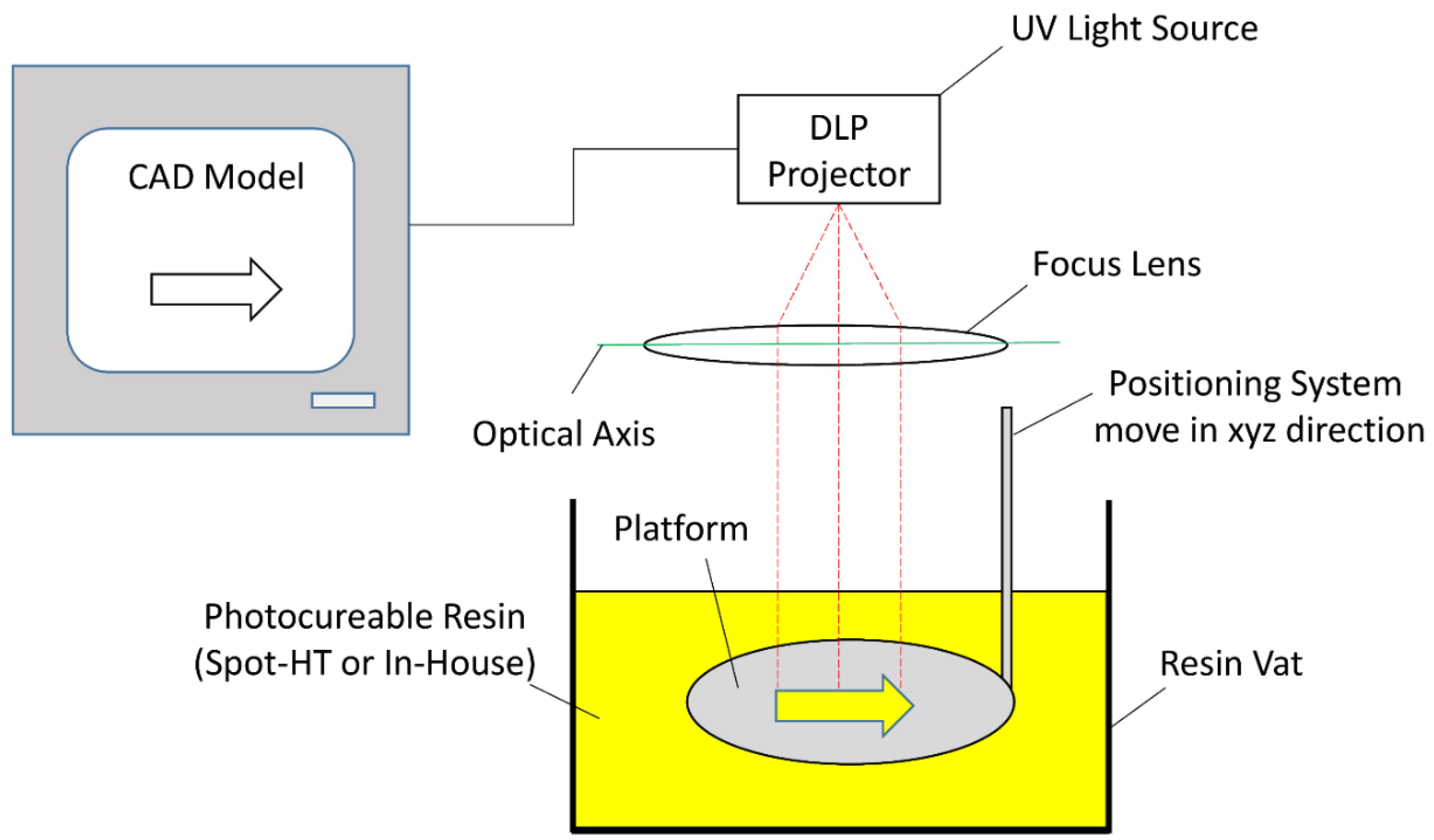
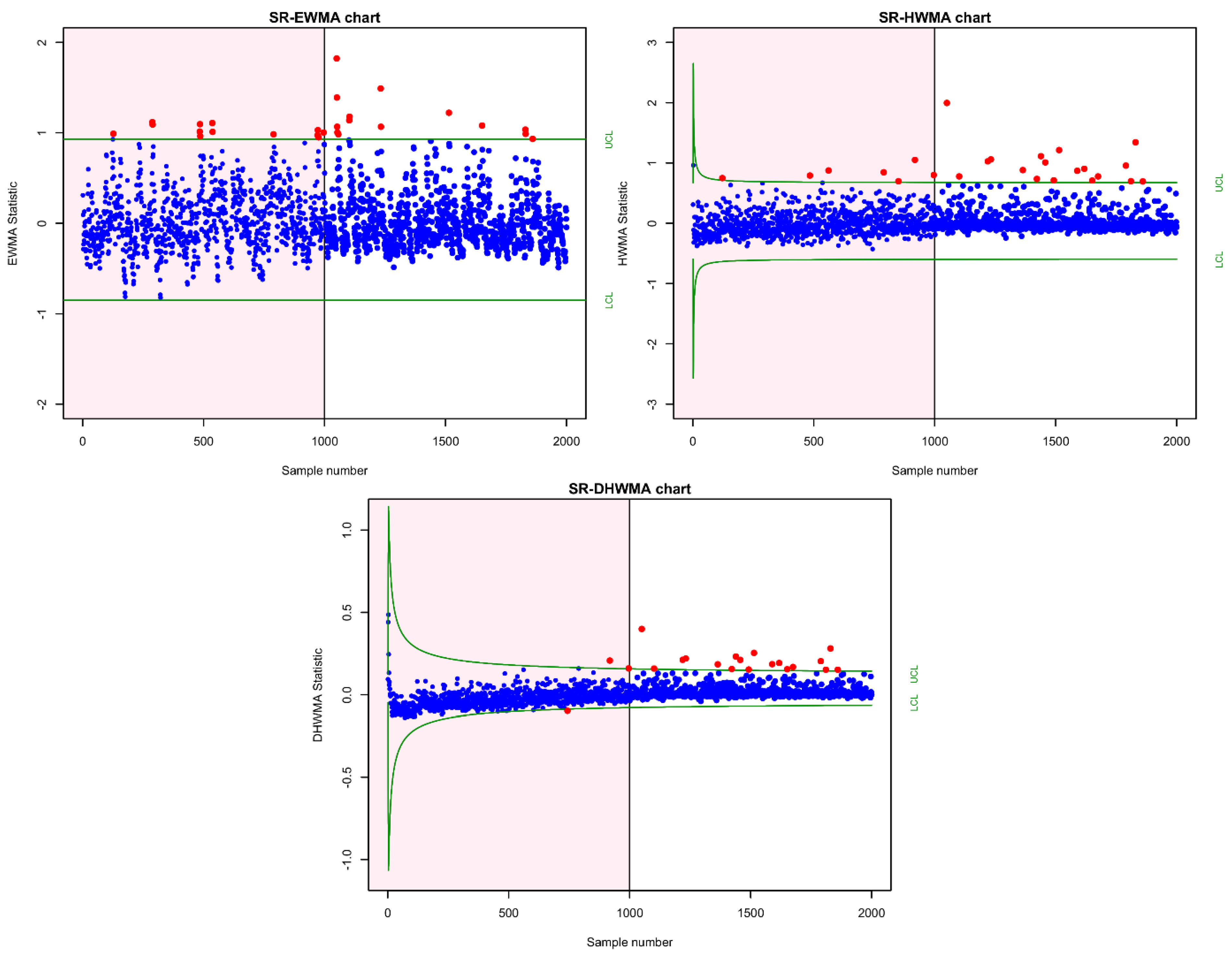
5. Illustrative Example

To demonstrate a potential implementation of the suggested control charts in a real-life state, we have adopted the example from Mahmood et al. [66]. The example relates to an additive manufacturing technology of stereolithography; the technique involves curing a photo-resistant resin by using an ultraviolet (UV) light source to manufacture prototypes and rapid tooling one layer at a time. As shown in Figure 1, the module consists of ultraviolet light, a vat of photocurable liquid resin and a monitoring system.

In the experiment, a commercialized resin called Spot-HT and an in-house resin were employed. However, determining acceptable parameters, such as light energy and cure depth, is essential. The issue of getting control or resistance has therefore been studied for both Spot-HT and in-house resins to examine whether the light intensity would increase or decrease from a UV light source of a specific intensity.

The two datasets are retrieved, each with 1000 sample points. The first dataset concerns the count of 3D faulty items for in-house resin stuff against light intensity, while the second dataset deals with the count of 3D faulty items for Spot-HT resin stuff against light intensity. In the analysis, the first dataset is taken as IC data, and the second dataset is deemed as OOC data. Further, the count of faulty items is treated as regressand $\left(y\right)$, with light intensity acting as a regressor $\left(x\right)$. The regressand $\left(y\right)$ in IC data and OOC data follows a Poisson distribution with rate parameters equal to 2.166 and 2.516, respectively. Moreover, the model’s fit was evaluated by using the Chi-squared goodness of fit test, and the Poisson distribution is found to be the best-fitted distribution, according to ${\chi }^2=2.865$ with p-value $=0.72$ for IC data and ${\chi }^2=2.516$ with p-value $=0.18$ for OOC data. Hence, we ran a Poisson regression model between the count of faulty items and light intensity for both datasets. The following are the models:

$$\mathrm{IC} \mathrm{Model}: y=e^{-5.846+0.841\left(x\right)},$$

(14)

$$\mathrm{OOC} \mathrm{Model}: y=e^{-6.540+0.813\left(x\right)},$$

(15)

It is seen from the simulation study that standardized residuals-based charts are more powerful charts; hence, the application is limited to SR-EWMA, SR-HWMA and SR-DHWMA charts for brevity. Control charting constants against $AR{L}_0=200$ are computed by following Section 4.2. It should be mentioned that the bootstrapping method is used, and at $\lambda =0.25$, the values are obtained as $L_{E1}=L_{E2}=2.7$, $L_{h1}=L_{h2}=3.2$ and $L_{dh1}=L_{dh2}=2.2$.

The plots of the SR-EWMA, SR-HWMA and SR-DHWMA charts that have been implemented are shown in Figure 2. To distinguish the IC and OOC panes, the IC pane has a pink shade, whilst the OOC pane has a white shaded region. It is perceived that the SR-EWMA chart has found 14 OOC signals, while both SR-HWMA and SR-DHWMA charts have detected 18 signals. According to this finding, the SR-HWMA and SR-DHWMA charts have superior detection ability in contrast with the SR-EWMA chart.

6. Summary, Conclusions and Recommendations

In this modern era, high-quality systems have been implanted in the manufacturing processes, leading to high-quality products in the markets. The control charts are useful devices for keeping track of a process’s quality. Control charts for the response variable are usually generated without taking the covariate into consideration that might be helpful in monitoring. A variety of linear profiling methodologies have been proposed in several research to investigate the relationship between the response variable and covariate but with the assumption of normality. In some processes, the quality characteristic might be well modeled by Poisson distribution (e.g., the number of breaks or the number of defects, the number of price changes, the number of accidents and the number of cases of a certain disease). To attain better outcomes in such instances, a novel technique based on a generalized linear model (GLM) that provides multiple distribution possibilities for response variables is necessary. This work produced GLM-based HWMA and DHWMA kinds of charts for monitoring count processes, using the deviance residuals and standardized residuals of the Poisson regression model. Under different sorts of alterations, the devised monitoring methods and previous control charts (originated from residuals) are assessed. The charts created from standardized residuals (i.e., SR-EWMA, SR-HWMA and SR-DHWMA) have been found to be more effective for shifts in the process mean.

Furthermore, the SR-DHWMA chart has been found to be more successful than the SR-EWMA and SR-HWMA structures regarding ARL and SDRL. An implementation of the suggested techniques is also presented by using an actual dataset pertaining to the additive manufacturing process where the proposals offered promising outcomes. The findings of the study may be helpful for quality engineers on appropriate and effective adoption of light intensity from a UV light source to prevent fault items in additive manufacturing process. The suggested monitoring methods are the quick ways to detect small changes in the process and can be used for monitoring and controlling the processes in the field of environmental sciences, epidemiology, healthcare, economics, highway safety surveillance, textile industry, etc. For instance, in the semiconductor industry, following fabrication, each die on a wafer is subjected to a series of tests until one fails or all tests pass, whatever comes first. The proposed schemes may guide the industry in taking effective steps to control the failures by considering other crucial factors, such as gas flow, exhaust and temperature.

For future studies, we recommend examining the effect of parameter estimation; considering two or even more covariates when estimating the Poisson parameter, ${\mu }_j$; extending the proposals to the latest monitoring schemes, such as mixed EWMA–CUSUM, mixed CUSUM–EWMA; and moving average structures.

References

1. Adegoke, N.A.; Abbasi, S.A.; Dawod, A.B.; Pawley, M.D. Enhancing the performance of the EWMA control chart for monitoring the process mean using auxiliary information. Qual. Reliab. Eng. Int. 2019, 35, 920–933. [Google Scholar] [CrossRef]
2. Mahmood, T. Generalized linear model based monitoring methods for high-yield processes. Qual. Reliab. Eng. Int. 2020, 36, 1570–1591. [Google Scholar] [CrossRef]
3. Adegoke, N.A.; Smith, A.N.; Anderson, M.J.; Sanusi, R.A.; Pawley, M.D. Efficient homogeneously weighted moving average chart for monitoring process mean using an auxiliary variable. IEEE Access 2019, 7, 94021–94032. [Google Scholar] [CrossRef]
4. Alevizakos, V.; Koukouvinos, C. A double progressive mean control chart for monitoring Poisson observations. J. Comput. Appl. Math. 2020, 373, 112232. [Google Scholar] [CrossRef]
5. Montgomery, D.C. Introduction to Statistical Quality Control, 6th ed.; John Wiley & Sons: New York, NY, USA, 2009. [Google Scholar]
6. Khoo, M.B. Poisson moving average versus c chart for nonconformities. Qual. Eng. 2004, 16, 525–534. [Google Scholar] [CrossRef]
7. Borror, C.M.; Champ, C.W.; Rigdon, S.E. Poisson EWMA control charts. J. Qual. Technol. 1998, 30, 352–361. [Google Scholar] [CrossRef]
8. Gan, F. Monitoring Poisson observations using modified exponentially weighted moving average control charts. Commun. Stat. Simul. Comput. 1990, 19, 103–124. [Google Scholar] [CrossRef]
9. Testik, M.C.; McCullough, B.; Borrar, C.M. The effect of estimated parameters on Poisson EWMA control charts. Qual. Technol. Quant. Manag. 2006, 3, 513–527. [Google Scholar] [CrossRef]
10. Zhang, L.; Govindaraju, K.; Lai, C.; Bebbington, M. Poisson DEWMA control chart. Commun. Stat. Simul. Comput. 2003, 32, 1265–1283. [Google Scholar] [CrossRef]
11. Shu, L.; Jiang, W.; Wu, Z. Exponentially weighted moving average control charts for monitoring increases in Poisson rate. IIE Trans. 2012, 44, 711–723. [Google Scholar] [CrossRef]
12. Yamauchi, T.; Lee Ho, L. Control charts for monitoring the ratio of two poisson rates. Qual. Reliab. Eng. Int. 2020, 36, 214–230. [Google Scholar] [CrossRef]
13. Weiß, C.H. Detecting mean increases in Poisson INAR (1) processes with EWMA control charts. J. Appl. Stat. 2011, 38, 383–398. [Google Scholar] [CrossRef]
14. Zhou, Q.; Zou, C.; Wang, Z.; Jiang, W. Likelihood-based EWMA charts for monitoring Poisson count data with time-varying sample sizes. J. Am. Stat. Assoc. 2012, 107, 1049–1062. [Google Scholar] [CrossRef]
15. Zhou, Q.; Shu, L.; Jiang, W. One-sided EWMA control charts for monitoring Poisson processes with varying sample sizes. Commun. Stat. Simul. Comput. 2016, 45, 6112–6132. [Google Scholar] [CrossRef]
16. Sheu, S.-H.; Chiu, W.-C. Poisson GWMA control chart. Commun. Stat. Simul. Comput. 2007, 36, 1099–1114. [Google Scholar] [CrossRef]
17. Chiu, W.C.; Sheu, S.H. Fast initial response features for Poisson GWMA control charts. Commun. Stat. Simul. Comput. 2008, 37, 1422–1439. [Google Scholar] [CrossRef]
18. Abujiya, M.A.R.; Abbasi, S.A.; Riaz, M. A new EWMA control chart for monitoring Poisson observations. Qual. Reliab. Eng. Int. 2016, 32, 3023–3033. [Google Scholar] [CrossRef]
19. Lucas, J.M. Counted data CUSUM’s. Technometrics 1985, 27, 129–144. [Google Scholar] [CrossRef]
20. White, C.H.; Bert Keats, J.; Stanley, J. Poisson cusum versus c chart for defect data. Qual. Eng. 1997, 9, 673–679. [Google Scholar] [CrossRef]
21. Abujiya, M.; Ramat, A. New cumulative sum control chart for monitoring Poisson processes. IEEE Access 2017, 5, 14298–14308. [Google Scholar] [CrossRef]
22. Jiang, W.; Shu, L.; Tsui, K.-L. Weighted CUSUM control charts for monitoring Poisson processes with varying sample sizes. J. Qual. Technol. 2011, 43, 346–362. [Google Scholar] [CrossRef]
23. Abbasi, S.A. Poisson progressive mean control chart. Qual. Reliab. Eng. Int. 2017, 33, 1855–1859. [Google Scholar] [CrossRef]
24. Chiu, J.-E.; Kuo, T.-I. Attribute control chart for multivariate Poisson distribution. Commun. Stat. Simul. Comput. 2007, 37, 146–158. [Google Scholar] [CrossRef]
25. He, S.; He, Z.; Wang, G.A. CUSUM control charts for multivariate Poisson distribution. Commun. Stat. Simul. Comput. 2014, 43, 1192–1208. [Google Scholar] [CrossRef]
26. Laungrungrong, B.; Borror, C.M.; Montgomery, D.C. EWMA control charts for multivariate Poisson-distributed data. Int. J. Qual. Eng. Technol. 2011, 2, 185–211. [Google Scholar] [CrossRef]
27. Raza, M.A.; Aslam, M. Design of control charts for multivariate Poisson distribution using generalized multiple dependent state sampling. Qual. Technol. Quant. Manag. 2019, 16, 629–650. [Google Scholar] [CrossRef]
28. Amiri, A.; Koosha, M.; Azhdari, A. Profile monitoring for Poisson responses. In Proceedings of the 2011 IEEE International Conference on Industrial Engineering and Engineering Management, Singapore, 6–9 December 2011; pp. 1481–1484. [Google Scholar]
29. Maleki, M.R.; Castagliola, P.; Amiri, A.; Khoo, M.B. The effect of parameter estimation on phase II monitoring of poisson regression profiles. Commun. Stat. Simul. Comput. 2019, 48, 1964–1978. [Google Scholar] [CrossRef]
30. Kuo, T.; Chiu, J. Regression-based limits for multivariate Poisson control chart. In Proceedings of the 2008 IEEE International Conference on Industrial Engineering and Engineering Management, Singapore, 8–11 December 2008; pp. 2051–2055. [Google Scholar]
31. Wen, H.; Liu, L.; Yan, X. Regression-adjusted Poisson EWMA control chart. Qual. Reliab. Eng. Int. 2021, 37, 1956–1964. [Google Scholar] [CrossRef]
32. Alencar, A.P.; Lee Ho, L.; Albarracin, O.Y.E. CUSUM control charts to monitor series of negative binomial count data. Stat. Methods Med. Res. 2017, 26, 1925–1935. [Google Scholar] [CrossRef] [PubMed]
33. Amin, M.; Mahmood, T.; Kinat, S. Memory type control charts with inverse-Gaussian response: An application to yarn manufacturing industry. Trans. Inst. Meas. Control. 2021, 43, 656–678. [Google Scholar] [CrossRef]
34. Kinat, S.; Amin, M.; Mahmood, T. GLM-based control charts for the inverse Gaussian distributed response variable. Qual. Reliab. Eng. Int. 2020, 36, 765–783. [Google Scholar] [CrossRef]
35. Mahmood, T.; Xie, M. Models and monitoring of zero-inflated processes: The past and current trends. Qual. Reliab. Eng. Int. 2019, 35, 2540–2557. [Google Scholar] [CrossRef]
36. Urbieta, P.; Lee, H.O.L.; Alencar, A. CUSUM and EWMA control charts for negative binomial distribution. Qual. Reliab. Eng. Int. 2017, 33, 793–801. [Google Scholar] [CrossRef]
37. Park, K.; Jung, D.; Kim, J.M. Control charts based on randomized quantile residuals. Appl. Stoch. Models Bus. Ind. 2020, 36, 716–729. [Google Scholar] [CrossRef]
38. Mammadova, U.; Özkale, M.R. Profile monitoring for count data using Poisson and Conway–Maxwell–Poisson regression-based control charts under multicollinearity problem. J. Comput. Appl. Math. 2021, 388, 113275. [Google Scholar] [CrossRef]
39. Marcondes Filho, D.; Sant’Anna, A.M.O. Principal component regression-based control charts for monitoring count data. Int. J. Adv. Manuf. Technol. 2016, 85, 1565–1574. [Google Scholar] [CrossRef]
40. Park, K.; Kim, J.M.; Jung, D. GLM-based statistical control r-charts for dispersed count data with multicollinearity between input variables. Qual. Reliab. Eng. Int. 2018, 34, 1103–1109. [Google Scholar] [CrossRef]
41. Jamal, A.; Mahmood, T.; Riaz, M.; Al-Ahmadi, H.M. GLM-Based Flexible Monitoring Methods: An Application to Real-Time Highway Safety Surveillance. Symmetry 2021, 13, 362. [Google Scholar] [CrossRef]
42. Skinner, K.R.; Montgomery, D.C.; Runger, G.C. Generalized linear model-based control charts for discrete semiconductor process data. Qual. Reliab. Eng. Int. 2004, 20, 777–786. [Google Scholar] [CrossRef]
43. Skinner, K.R.; Montgomery, D.C.; Runger, G.C. Process monitoring for multiple count data using generalized linear model-based control charts. Int. J. Prod. Res. 2003, 41, 1167–1180. [Google Scholar] [CrossRef]
44. Asgari, A.; Amiri, A.; Niaki, S.T.A. A new link function in GLM-based control charts to improve monitoring of two-stage processes with Poisson response. Int. J. Adv. Manuf. Technol. 2014, 72, 1243–1256. [Google Scholar] [CrossRef]
45. Abbas, N.; Riaz, M.; Ahmad, S.; Abid, M.; Zaman, B. On the efficient monitoring of multivariate processes with unknown parameters. Mathematics 2020, 8, 823. [Google Scholar] [CrossRef]
46. Abid, M.; Mei, S.; Nazir, H.Z.; Riaz, M.; Hussain, S. A mixed HWMA-CUSUM mean chart with an application to manufacturing process. Qual. Reliab. Eng. Int. 2020, 37, 618–631. [Google Scholar] [CrossRef]
47. Abid, M.; Shabbir, A.; Nazir, H.Z.; Sherwani, R.A.K.; Riaz, M. A double homogeneously weighted moving average control chart for monitoring of the process mean. Qual. Reliab. Eng. Int. 2020, 36, 1513–1527. [Google Scholar] [CrossRef]
48. Adegoke, N.A.; Abbasi, S.A.; Smith, A.N.; Anderson, M.J.; Pawley, M.D. A multivariate homogeneously weighted moving average control chart. IEEE Access 2019, 7, 9586–9597. [Google Scholar] [CrossRef]
49. Raza, M.A.; Nawaz, T.; Han, D. On designing distribution-free homogeneously weighted moving average control charts. J. Test. Eval. 2020, 48, 3154–3171. [Google Scholar] [CrossRef]
50. Riaz, M.; Abbasi, S.A.; Abid, M.; Hamzat, A.K. A New HWMA Dispersion Control Chart with an Application to Wind Farm Data. Mathematics 2020, 8, 2136. [Google Scholar] [CrossRef]
51. Riaz, M.; Abid, M.; Shabbir, A.; Nazir, H.Z.; Abbas, Z.; Abbasi, S.A. A non-parametric double homogeneously weighted moving average control chart under sign statistic. Qual. Reliab. Eng. Int. 2020, 37, 1544–1560. [Google Scholar] [CrossRef]
52. Yates, R.D.; Goodman, D.J. Probability and Stochastic Processes: A Friendly Introduction for Electrical and Computer Engineers, 2nd ed.; John Wiley & Sons: Hoboken, NJ, USA, 2014. [Google Scholar]
53. Haight, F.A. Handbook of the Poisson Distribution; John Wiley & Sons: New York, NY, USA, 1967. [Google Scholar]
54. McCullagh, P.; Nelder, J.A. Generalized Linear Models, 2nd ed.; Chapman and Hall: London, UK, 1989. [Google Scholar]
55. Pierce, D.A.; Schafer, D.W. Residuals in generalized linear models. J. Am. Stat. Assoc. 1986, 81, 977–986. [Google Scholar] [CrossRef]
56. Abbas, N.; Abujiya, M.A.R.; Riaz, M.; Mahmood, T. Cumulative sum chart modeled under the presence of outliers. Mathematics 2020, 8, 269. [Google Scholar] [CrossRef] [Green Version]
57. Ali, S.; Abbas, Z.; Nazir, H.Z.; Riaz, M.; Zhang, X.; Li, Y. On Designing Non-Parametric EWMA Sign Chart under Ranked Set Sampling Scheme with Application to Industrial Process. Mathematics 2020, 8, 1497. [Google Scholar] [CrossRef]
58. Chen, J.-H.; Lu, S.-L. A New Sum of Squares Exponentially Weighted Moving Average Control Chart Using Auxiliary Information. Symmetry 2020, 12, 1888. [Google Scholar] [CrossRef]
59. Abbas, N.; Riaz, M.; Does, R.J. Mixed exponentially weighted moving average–cumulative sum charts for process monitoring. Qual. Reliab. Eng. Int. 2013, 29, 345–356. [Google Scholar] [CrossRef]
60. Capizzi, G.; Masarotto, G. An adaptive exponentially weighted moving average control chart. Technometrics 2003, 45, 199–207. [Google Scholar] [CrossRef] [Green Version]
61. Li, Z.; Xie, M.; Zhou, M. Rank-based EWMA procedure for sequentially detecting changes of process location and variability. Qual. Technol. Quant. Manag. 2018, 15, 354–373. [Google Scholar] [CrossRef]
62. Lucas, J.M.; Saccucci, M.S. Exponentially weighted moving average control schemes: Properties and enhancements. Technometrics 1990, 32, 1–12. [Google Scholar] [CrossRef]
63. Riaz, S.; Riaz, M.; Hussain, Z.; Abbas, T. Monitoring the performance of Bayesian EWMA control chart using loss functions. Comput. Ind. Eng. 2017, 112, 426–436. [Google Scholar] [CrossRef]
64. Abbas, N. Homogeneously weighted moving average control chart with an application in substrate manufacturing process. Comput. Ind. Eng. 2018, 120, 460–470. [Google Scholar] [CrossRef]
65. Alevizakos, V.; Chatterjee, K.; Koukouvinos, C. The extended homogeneously weighted moving average control chart. Qual. Reliab. Eng. Int. 2021, 37, 2134–2155. [Google Scholar] [CrossRef]
66. Mahmood, T.; Iqbal, A.; Abbasi, S.A.; Amin, M. Efficient GLM-based control charts for Poisson processes. Qual. Reliab. Eng. Int. 2021. [Google Scholar] [CrossRef]
Figure 1. Basic working principle of projection based stereolithography.
Symmetry 14 00122 g001
Figure 2. Implementation of SR-EWMA, SR-HWMA and SR-DHWMA charts on 3D defects dataset.
Symmetry 14 00122 g002