Abstract
This article deals with symmetrical data that can be modelled based on Gaussian distribution. We consider a class of partially linear additive spatial autoregressive (PLASAR) models for spatial data. We develop a Bayesian free-knot splines approach to approximate the nonparametric functions. It can be performed to facilitate efficient Markov chain Monte Carlo (MCMC) tools to design a Gibbs sampler to explore the full conditional posterior distributions and analyze the PLASAR models. In order to acquire a rapidly-convergent algorithm, a modified Bayesian free-knot splines approach incorporated with powerful MCMC techniques is employed. The Bayesian estimator (BE) method is more computationally efficient than the generalized method of moments estimator (GMME) and thus capable of handling large scales of spatial data. The performance of the PLASAR model and methodology is illustrated by a simulation, and the model is used to analyze a Sydney real estate dataset.
1. Introduction
Spatial econometrics models are frequently proposed to analyze spatial data that arise in many disciplines such as urban, real estate, public, agricultural, environmental economics and industrial organizations. These models address relationships across geographic observations caused by spatial autocorrelation in cross-sectional or longitudinal data. Spatial econometrics models have a long history in both econometrics and statistics. Early developments and relevant surveys can be found in Cliff and Ord [1], Anselin [2], Case [3], Cressie [4], LeSage [5,6], Anselin and Bera [7].
Among spatial econometrics models, spatial autoregressive (SAR) models [1] have gained much attention by theoretical econometricians and applied researchers. Many approaches have been used to estimate the SAR models, which include the maximum likelihood estimator (MLE) [8], the generalized method of moment estimator (GMME) [9], and the quasi-maximum likelihood estimator (QMLE) [10]. However, these methods mainly focused on parametric SAR models, which are frequently assumed to be linear, few researchers have explicitly examined non-/semi-parametric SAR models. Indeed, it has been confirmed that a lot of economic variables exhibit highly nonlinear relationships on the dependent variables [11,12,13]. Neglecting the latent nonlinear functional forms often results in an inconsistent estimation of the parameters and misleading conclusions [14].
Although many empirical studies and econometric analyses applying the parametric SAR models ignore latent nonlinear relationships, several nonlinear forms [15,16,17,18] have been considered. Nevertheless, the nonlinear parametric SAR models can at most supply certain protection against some specific nonlinear functional forms. Since the nonlinear function is unknown, it is unavoidable to assume the risk of misspecifying the nonlinear function. As nonparametric techniques advance, the advantage of nonparametric SAR models are often used to model nonlinear economic relationships. However, nonparametric components are only suitable for low dimensional covariates, otherwise the “curse of dimensionality” [19] problem is often encountered. Some nonparametric dimension-reduction tools have been considered to address this problem, for example, single-index model [20], partially linear model [21], the additive model [22], varying-coefficient model [23], among others. In recent years, many researchers have started using the advantage of semiparametric modeling in spatial econometrics. For example, Su and Jin [14] proposed the QMLE for semiparametric partially linear SAR models; Su [24] discussed GMME of semiparametric SAR models; Chen et al. [25] studied a Bayesian method for the semiparametric SAR models; Wei and Sun [26] considered GMME for the space-varying coefficients of a spatial model; Krisztin [27] investigated a novel Bayesian semiparametric estimation for the penalized spline SAR models; Krisztin [28] presented a genetic-algorithms for a nonlinear SAR model; Du et al. [29] established GMME of PLASAR models; Chen and Cheng [30] developed a GMME of a partially linear additive spatial error model.
Semiparametric models have received much attention from both econometrics and statistics owing to the explanatory of the parameters and the flexibility of nonparameters. The partially linear additive (PLA) model is probably one of the most popular among the various semiparametric models. As they can not only avoid the “curse of dimensionality” phenomenon encountered in nonparametric regression but also provide a more flexible structure than the generalized linear models. As a result, the PLA models provide good equilibrium between flexibility of the additive model and interpretation of the partially linear model. Many researchers have considered many approaches to analyze such models: local linear method [31], spline estimation [32,33,34], quantile regression [35,36,37,38], variable selection [39,40,41,42], etc. Characterizing the flexibility of nonparametric forms and attempting to explain the potential nonlinearity of PLASAR models are unique challenges faced by analysts of spatial data.
Combining PLA models with SAR models, we consider a class of PLASAR models for spatial data to capture the linear and nonlinear effects between the related variables in addition to spatial dependence between the neighbors in this article. We specify the prior of all unknown parameters, which led to a proper posterior distribution. The posterior summaries are obtained via MCMC tools. We develop an improved Bayesian method with free-knot splines [43,44,45,46,47,48,49,50,51], along with MCMC techniques to estimate unknown parameters, use a spline approach to approximate the nonparametric functions, and design a Gibbs sampler to explore the joint posterior distributions. Treating the number and the positions of knots as random variables can make the model spatially adaptive is an attractive feature of Bayesian free-knot splines [45,46]. In order to improve the rapidly-convergent performance of our algorithm, we further modify the movement step of Bayesian free-knots splines such that all knots can be repositioned in each iteration instead of only one knot moving. Finally, the performance of the PLASAR model and methodology is illustrated by a simulation, and they are used to analyze real data.
The rest of this paper is organized as follows. In Section 2, we propose the PLASAR model to analyze spatial data and discuss the proposed model’s identifiability condition, then acquire the likelihood function by fitting the nonparametric functions with a Bayesian free-knots splines approach. To provide a Bayesian framework, we specify the priors for the unknown parameters, derive the full conditional posterior distributions of the unknown parameters, modify the movement step of the Bayesian free-knots splines approach to accelerate the convergent performance of our algorithm, and describe the detailed sampling algorithm in Section 3. The applicability and practicality of the PLASA model and methodology for spatial data are evaluated by a simulation study, and the model is used to analyze a real dataset in Section 4. Section 5 concludes the paper with a summary.
2. Methodology
2.1. Model
We begin with the PLASAR model that is defined as
where and are covariate vectors, is a response variable, is a specified constant spatial weight, is unknown univariate nonparametric function for , is vector of the unknown parameters, the unknown spatial parameter reflects the spatial autocorrelation between the neighbors with stability condition , and ’s are mutually independent and identically distributed normal with zero mean and variance . In order to ensure model identifiability of the nonparametric function, it is often assumed that the condition for .
2.2. Likelihood
We plan on approximating unknown functions in (1) by free-knot splines for . Assuming that has a polynomial spline of degree with order interior knots with , i.e.,
where , the vector of spline basis is determined by the knot vector , the spline coefficients is a vector, and
are boundary knots for . Let and . To achieve identification, we set , which is written as . Denote , then the constraint becomes .
It follows that the model (1) can be equivalent to
where and . Then the matrix form of the model (1) can be represented as
where , , , is an specified constant spatial wight matrix, , and is an matrix with as its ith row.
The likelihood function for the PLASAR model is proportional to
where , , is vector of regression coefficient, is an matrix, , and is an identity matrix of order n.
3. Bayesian Estimation
In this section, we consider a Bayesian free-knots splines approach with MCMC techniques to analyze the PLASAR model. We begin with the specification of the prior distributions of all unknown parameters, then the derivations of posterior distributions and the narration of the detailed sampling scheme for all of the unknown parameters. Meanwhile, we modify the movement step of Bayesian free-knots splines approach so that all the knots can be repositioned in each iteration.
3.1. Priors
As we will consider a Bayesian approach with free-knots splines to analyze the PLASAR models, all unknown parameters are assigned prior distributions. Note that besides regression coefficient vectors , the spatial autocorrelation coefficient and the quantities , the number of knots and location of knots also need prior distributions in the sense that they are random variables in the Bayesian approach with free-knot splines. We avoid the use of improper prior distributions to prevent improper joint posterior distributions.
For , we followed Poon and Wang [49] by puting a Poisson prior with mean for number of the knots
and a conditional flat prior for knot location
where , and are defined in (3).
We set a conjugate normal inverse-gamma prior for the unknown parameters , which is a composite of inverse-Gamma prior distributions for
where and are hyperparameters; a conditional normal prior distribution with mean vector and covariance matrix for
and a conditional normal prior distribution with mean vector and covariance matrix for with the constraint as follows:
for . In order to improve the robustness of our method, we choose an inverse-gamma prior
for , where and are pre-specified hyper-parameters. Throughout this article we set to obtain a Cauchy distribution of and assign and to acquire a highly dispersed inverse gamma prior on for .
In addition, we follow LeSage and Pace [52] by eliciting a uniform prior for the spatial autocorrelation coefficient
where and are the maximum and minimum eigenvalues of the standardized spatial weight matrix W, respectively.
Therefore, the joint priors of all of the quantities are defined as
where is a hyperparameters vector. For computational convenience, we have treated the hyperparameter vector as a unknown parameter vector.
3.2. The Full Conditional Posterior Distributions of Unknown Quantities
Since the joint posterior distribution of the quantities is very complicated, it is difficult to generate samples directly. To solve this problem, we derive the full conditional posterior distributions of unknown quantities, modify the movement step of Bayesian free-knots splines to speed up the convergence, and describe the detailed sampling method in our algorithm.
It follows from the likelihood function (4) and the joint priors (5) that the conditional posterior distribution of given the remaining unknown parameters is proportional to
It is not easy to directly simulate from (6), which does not have the form of any standard density function. Therefore, we prefer the Metropolis–Hastings algorithm [53,54] to solve this difficulty: draw from a truncated Cauchy distribution with location and scale on , where is treated as a tuning parameter; and accept the candidate value with probability
where
From likelihood function (4) and priors (5), we can see that given , the joint posterior of is given by
where , , , , , and , which gives rise to a marginal posterior distribution
It is easy to see from (8) that
where , , , and are with excluded, respectively.
It follows from (7) that the approach of composition [55] can be used to generate from a conditional inverse-gamma posterior
and to sample from a conditional normal posterior
It follows from (11) that
where , , , and
for To achieve identification, we focus on the constraint , which should be imposed on . According to Panagiotelis and Smith [56], drawing from (13) is equivalent to drawing from a normal distribution with mean vector and covariance matrix , then is transformed to by
As it is convenient to sample from the conditional posterior (10), (12) and (13), we concentrate on sampling from (9). A sampling method is applied, in which the original Bayesian free-knots spline [43,44,45,46,47,48,49,50,51] is used as a reversible-jump sampler [57]. It includes three types of movement: the deletion, the addition and the movement of only one knot [48]. We keep the first two move-types unchanged but improve the movement step through the hit-and-run algorithm [58] so that all the knots can be repositioned in each iteration instead of only one knot: for select a dimension direction vector randomly, and define
generate from a Cauchy distribution with location 0 and scale truncated on , where acts as a tuning parameter; assign and reorder all of the knots. The proposed number and positions of knots are finally accepted with probability
where and correspond to and in the candidate posterior, respectively, and the factor
3.3. Sampling Scheme
The Bayesian estimate of is obtained by observations generated from the posterior of all unknown quantities by running the Gibbs sampler. Moreover, simulating from (13) is challenging and nonstandard, and the parameter space on the constraint for . According to Panagiotelis and Smith [56], it is equivalent that is transformed to by (14). The MCMC sampling algorithm (Algorithm 1) is described in the following manner.
| Algorithm 1 The MCMC sampling algorithm. |
| Input: Samples . Initialization: Initialize in the MCMC algorithm, where the unknown parameters are generated from the priors, respectively. MCMC iterations: Given the current state of successively, draw from , for The detailed MCMC sampling cycles are outlined in the following manner. (a) Generate from ; (b) Generate from ; (c) Generate from ; (d) Generate from for ; (e) Generate from , and adjust according to (14) for ; (f) Generate from for ; (g) Generate from . Output: The MCMC sampling from the conditional posteriors of . |
4. Empirical Illustrations
We demonstrate the performance of the PLSISAR model and methodology by a simulation and use them to analyze a real data. We set the Rook weight matrix [2] and the Case weight matrix [3] to examine the influence of the spatial weight matrix W. The Rook weight matrix is sampled from Rook contiguity in [59] by randomly allocating the n spatial units on a lattice of () squares, finding the neighbors for the unit, and then row normalizing. Meanwhile, we generated the Case weight matrix from the spatial scenario in [3] with m members in a district and r districts, and each neighbor of a member in each district given equal weight [10], where ⨂ is the Kronecker product, and is an m-dimensional vector.
4.1. Simulation
Consider the following PLSISAR models:
where follows a bivariate standard normal distribution, is a bivariate vector, where and are mutually independent and follow uniform distributions on and , respectively. The nonparametric functions and , , the parameters are assumed as and two cases of variance , respectively. We consider three different cases of spatial parameters , which represent the spatial dependence of the response from weak to strong. The sample size of the Case weight matrix and the Rook weight matrix is and , respectively.
In our computation, we run each simulation with 1000 replications, adopt a quadratic B-spline and set hyper-parameters and for . The initial state of the Markov chain of all unknown parameters is selected as follows. All unknown parameters are sampled from the respective priors by gradually decreasing or increasing the use of tuning parameters and for so that the acceptable rates are about 25%. For each replication, we generate 6000 sampled values and then delete the first 2000 sampled values as a burn-in period by running our MCMC sampling. Based on the last 4000 sampled values, we compute the corresponding average of 1000 replications as the posterior mean (mean), the 95% posterior credible intervals (95% CI), and standard error (SE). In addition, the standard derivations (SD) of the estimated posterior mean are calculate to compare them with the mean of the estimated posterior SE.
We evaluate the performance of nonparametric estimators by the integrated squared bias (Bias), the root integrated mean squared errors (SSE), the mean absolute deviation errors (MADE)
for , where mathematical expectations are estimated by their corresponding empirical version, and the integrations are performed applying a Riemannian sum approximation at 200 fixed grid points that are equally-spaced chosen from . From the model (1), the marginal effects are given by for . According to LeSage and Pace [52] suggestions, the mean of either the row sums or the column sums of the non-diagonal elements is used as the indirect effects, the mean of the diagonal elements is used as the direct effects, and the sum of the indirect and direct effects is taken as the total effects.
To check the convergence of our algorithm, we run five Markov chains corresponding to different starting values through the MCMC sampling algorithm to perform each replication. The sampled traces of some parameters and nonparametric functions on grid points are displayed in Figure 1. It is obvious that the five parallel sequences mix quite well. We compute the “potential scale reduction factor” [60] for all unknown parameters and nonparametric functions at 20 selected grid points. Figure 2 shows all the values of against the iteration numbers. According to the suggestion of Gelman and Rubin [60], it is easy to see that 2000 burn-in iterations are enough to make the MCMC algorithm converge as all the values of were less than 1.2.
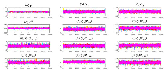
Figure 1.
Trace plots of five parallel Markov chains with different starting values for some parameters and nonparametric functions (only a replication with and is displayed).
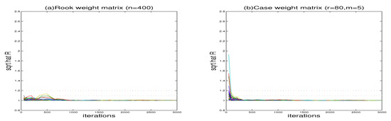
Figure 2.
The “potential scale reduction factor” for simulation results (the case of ).
The boxplots of the Bias values are displayed in Figure 3. Under the Rook weight matrix, the medians of which are and for , and and for , respectively. Under the Case weight matrix, the medians of which are and for , and and for , respectively. Figure 3 show the boxplots of the SEE values. Under the Rook weight matrix, the medians are and for , and and for , respectively. Under the Case weight matrix, the medians are and for , and and for , respectively. The results show that the Bias values and the SEE values of the nonparametric functions decrease with the increase in the sample size, indicating that the nonparametric estimation is convergent. It is evident that the weight matrix of Case and Rook can obtain a reasonable estimation effect.
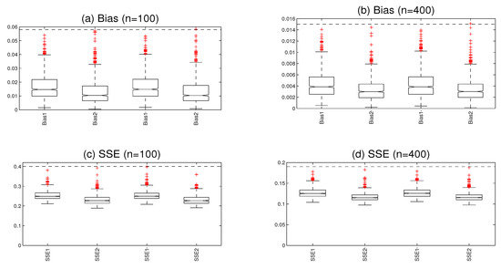
Figure 3.
The boxplots (a,b) display the integrated squared bias, the boxplots (c,d) display the root integrated mean squared errors. (The two panels on the left are based on the Rook weight matrix, and the two panels on the right are based on the Case weight matrix with ).
The estimation results are reported in Table 1. We observe that the mean values of all estimators are very close to the corresponding true values, and the mean value of SE is close to the respective SD. The results show that the parameter estimation and SE are precise. Meanwhile, the larger the sample sizes under the same weight matrix, the more precise the estimates are. The above experiences corresponding to different starting values have been repeated, and the results are similar. It implies that the MCMC sampling works well. Moreover, we find that the estimation effect of with the Case weight matrix is slightly better than that with Rook weight matrix under the same sample sizes. The possible main reason is that the performance of the Case weight matrix is superior to the Rook weight matrix under different variances . In addition, the general pattern of estimates reported in Table 1 is that all estimators impose a relatively bigger bias on the total effect when the same sample sizes have a strong positive spatial dependence. Figure 4 depicts the fitted functions, together with its 95% CI from a typical sample with and . The typical sample is selected in such a way that the SSE values are equal to the median in the 1000 replications. It is obvious that the fitted nonparametric functions are improving with increasing the sample size.

Table 1.
Simulation results of parametric estimation.
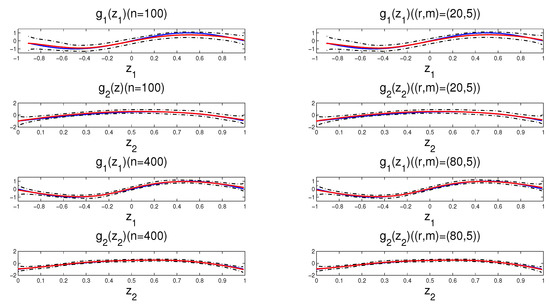
Figure 4.
The true functions (solid lines), the fitted functions (dotted lines) and their 95% CI (dot-dashed lines) for a typical sample (the left panel based on the Rook weight matrix and the right panel based on the Case weight matrix with ).
For comparison purposes, we use the Bayesian P-splines approach to approximate the nonparametric functions [61], where we assign a second-order random walk prior to the spline coefficients. The boxplots of MADE values with the Case weight matrix in Figure 5. In our method, the medians of MADE are , and for , and the medians of MADE are , and for , respectively, which are slightly smaller than the Bayesian P-splines approach. The results show that the Bayesian free knots splines approach is superior to the Bayesian P-splines approach in terms of fitting unknown nonparametric functions and computing time. Furthermore, we also compare the performance between the generalized method of moment estimator (GMME) in Du et al. [29] and the Bayesian MCMC estimator (BE) in our method. In order to evaluate the estimation effect of the nonparametric functions, we calculate the integrated squared bias (Bias) and the root integrated mean squared errors (SSE). Table 2 reports the results of the nonparameter estimation for GMME and BE (only a replication with is displayed). It is evident that the estimates are improving with increasing the sample size, the Bias of the BE estimates are slightly smaller than the Bias of the GMME, and the SSE of the BE estimates are very smaller than Bias of the GMME under the same sample size, showing that BE is better than GMME, although the latter can also obtain a reasonable estimation.
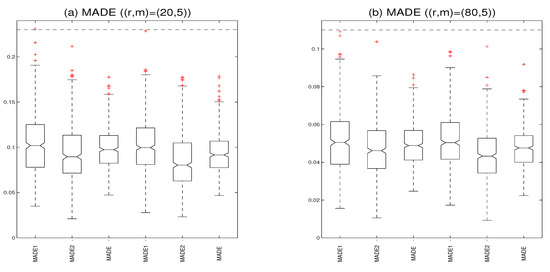
Figure 5.
The boxplots (a) display the mean absolute deviation errors with the Case weight matrix and (b) display the mean absolute deviation errors with the Case weight matrix (the three panels on the left are based on Bayesian free knots splines and the three panels on the right are based on Bayesian P-splines).
Table 2.
Simulation results of the nonparametric estimation.
4.2. Application
We use the proposed model and estimation methods to analyze the well-known Sydney real estate data. A detailed description of the data set can be found in Harezlak et al. [62]. The data set contains a total of 37,676 properties sold in the Sydney Statistical Division in the calendar year of 2001, which is available from the HRW package in R. We only focus on the last week of February to avoid the temporal issue, and there are 538 properties.
In this application, the house price (Price) is explained by four variables that include average weekly income (Income), levels of particulate matter with a diameter of less than a 10 micrometers level recorded at the air pollution monitoring station closest to the house (PM), lot size (LS), and distance from house to the nearest coastline location in kilometers (DC). On the one hand, Income and PM have a linear effect on the response Price. On the other hand, LS and DC have a nonlinear effect on the response Price. Meanwhile, logarithmic transformation is performed on all variables to alleviate the trouble caused by large gaps in the domain. In addition, all variables are transformed such that the marginal distribution is approximately a standard normal distribution. This motivates us to consider the PLASAR model:
where the response variable , , , , . Regarding the choice of the weight matrix, we use the Euclidean distance between any two houses to calculate the spatial weight matrix [63]. The spatial weight is
where is represented as the longitude and latitude of location. We apply a quadratic B-splines and assign hyperparameters for in our computation. We gradually decrease or increase the use of tuning parameters and such that the acceptable rates for updating and are around 25% for .
We generate 10,000 sampled values following a burn-in of 10,000 iterations and run the proposed Gibbs sampler five times with different initial states in each replication. Figure 6 plot the traces of some unknown parameters and nonparametric functions on grid points. It is obvious that the five parallel Markov chains mix well. We further calculate the “potential scale reduction factor” for each of the unknown parameters and nonparametric functions on 20 selected grid points, which are plotted in Figure 7. The result indicates that the Markov chains have converged within the first 10,000 burn-in iterations.
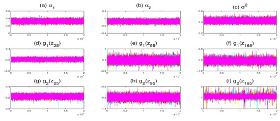
Figure 6.
Trace plots of five parallel Markov chains with different starting values for some parameters and nonparametric functions.
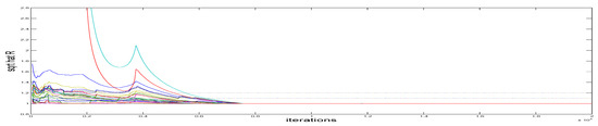
Figure 7.
The “potential scale reduction factor” for Sydney real estate data.
Table 3 lists the estimated parameters together with their SE and 95% CI, which show that the estimation of is 0.5548 with . It implies that there exists a significant and positive spatial relationship on the housing price. We find that two covaraites have significant effects on the housing price, and the effects of Income are positive, but PM is negative. The regression coefficient of Income is , which indicates that the Income has a positive effect on the housing price. Moreover, the regression coefficient of PM is , which reveals that the housing price would decrease as the PM increases.
Table 3.
Parametric estimation in the model (17) for Sydney real estate data.
Figure 8 depicts the fitted functions, together with its 95% CI, which look like two nonlinear functions. The curves show that has a local maximum 0.6184 at around and a local minimum 0.1557 at around , and has a local minimum −0.8224 at around . The results provide evidence that the significant effects of LS and DC on the housing price have a nonlinear S-shape and U-shape, respectively.
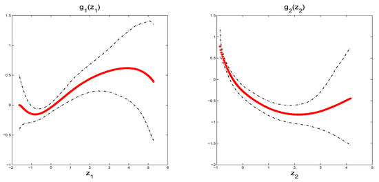
Figure 8.
The fitted functions (dotted lines) and their 95% CI (dot-dashed lines) in the model (17) for Sydney real estate data.
5. Summary
Spatial data are frequently encountered in practical applications and can be analyzed through the SAR model. To avoid some serious shortcomings of fully nonparametric models and reduce the high risk of misspecification of the traditional SAR models, we have considered PLASAR models for spatial data, which combine the PLA model and SAR model. In addition to spatial dependence between neighbors, it captures the linear and nonlinear effects between the related variables. We specify the prior of all unknown parameters, which led to a proper posterior distribution. The posterior summaries are obtained via the MCMC technique, and we have considered a fully Bayesian approach with free-knot splines to analyze the PLASAR model and design a Gibbs sampler to explore the full conditional posterior distributions. To obtain a rapidly-convergent algorithm, a modified Bayesian free-knot splines approach incorporated with powerful MCMC techniques is employed. We have illustrated that the finite sample of the proposed model and estimation method perform satisfactorily through a simulation study. The results show that the Bayesian estimator is efficient relative to the GMME, although the latter can also obtain reasonable estimations. Finally, the proposed model and methodology are applied to analyze real data.
This article focuses only on symmetrical data and the homoscedasticity of independent errors. Since spatial data cannot easily meet the conditions, it is fairly straightforward to analyze the proposed model and methodology to deal with spatial errors and heteroscedasticity. While we use PLASAR models to assess the linear and nonlinear effects of the covariates on the spatial response, the other models, such as partially linear single-index SAR models and partially linear varying-coefficient SAR models, can also be considered. Moreover, it would be interesting to develop a model selection method in which covariates are linear or nonlinear. We leave these topics for future research.
Author Contributions
Supervision, Z.C. and J.C.; software, Z.C.; methodology, Z.C.; writing—original draft preparation, Z.C.; writing—review and editing, Z.C. and J.C. Both authors have read and agreed to the published version of the manuscript.
Funding
This work was supported by the Natural Science Foundation of China (12001105), the Natural Science Foundation of Fujian Province (2020J01170), the Postdoctoral Science Foundation of China (2019M660156), the Program for Probability and Statistics: Theory and Application (No. IRTL1704), and the Program for Innovative Research Team in Science and Technology in Fujian Province University (IRTSTFJ).
Institutional Review Board Statement
Not applicable.
Informed Consent Statement
Not applicable.
Data Availability Statement
The data presented in this study are openly available in Reference [62].
Acknowledgments
The authors are most grateful to anonymous referees and the editors for their careful reading and insightful comments, who have helped to significantly improve this paper.
Conflicts of Interest
The authors declare no conflict of interest.
References
- Cliff, A.D.; Ord, J.K. Spatial Autocorrelation; Pion Ltd.: London, UK, 1973. [Google Scholar]
- Anselin, L. Spatial Econometrics: Methods and Models; Kluwer Academic Publisher: Dordrecht, The Netherlands, 1988. [Google Scholar]
- Case, A.C. Spatial patterns in householed demand. Econometrica 1991, 59, 953–965. [Google Scholar] [CrossRef] [Green Version]
- Cressie, N. Statistics for Spatial Data; John Wiley and Sons: New York, NY, USA, 1993. [Google Scholar]
- LeSage, J.P. Bayesian estimation of spatial autoregressive models. Int. Reg. Sci. Rev. 1997, 20, 113–129. [Google Scholar] [CrossRef]
- LeSage, J.P. Bayesian estimation of limited dependent variable spatial autoregressive models. Geogr. Anal. 2000, 32, 19–35. [Google Scholar] [CrossRef]
- Anselin, L.; Bera, A.K. Spatial dependence in linear regression models with an introduction to spatial econometrics. In Handbook of Applied Economics Statistics; Marcel Dekker: New York, NY, USA, 1998. [Google Scholar]
- Ord, J. Estimation methods for models of spatial interaction. J. Am. Stat. Assoc. 1975, 70, 120–126. [Google Scholar] [CrossRef]
- Kelejian, H.H.; Prucha, I.R. A generalized moments estimator for the autoregressive parameter in a spatial model. Int. Econ. Rev. 1999, 40, 509–533. [Google Scholar] [CrossRef] [Green Version]
- Lee, L.F. Asymptotic distribution of quasi-maximum likelihood estimators for spatial autoregressive models. Econometrica 2004, 72, 1899–1925. [Google Scholar] [CrossRef]
- Paelinck, J.H.P.; Klaassen, L.H.; Ancot, J.P.; Verster, A.C.P. Spatial Econometrics; Gower: Farnborough, UK, 1979. [Google Scholar]
- Basile, R.; Gress, B. Semi-parametric spatial auto-covariance models of regional growth behaviour in Europe. Rég. Dév. 2004, 21, 93–118. [Google Scholar] [CrossRef]
- Basile, R. Regional economic growth in Europe: A semiparametric spatial dependence approach. Pape. Reg. Sci. 2008, 87, 527–544. [Google Scholar] [CrossRef]
- Su, L.J.; Jin, S.N. Profile quasi-maximum likelihood estimation of partially linear spatial autoregressive models. J. Econom. 2010, 157, 18–33. [Google Scholar] [CrossRef]
- Baltagi, B.H.; Li, D. LM tests for functional form and spatial correlation. Int. Reg. Sci. Rev. 2001, 24, 194–225. [Google Scholar] [CrossRef]
- Pace, P.K.; Barry, R.; Slawson, V.C., Jr.; Sirmans, C.F. Simultaneous spatial and functional form transformation. In Advances in Spatial Econometrics; Anselin, L., Florax, R., Rey, S.J., Eds.; Springer: Berlin, Germany, 2004; pp. 197–224. [Google Scholar]
- van Gastel, R.A.J.J.; Paelinck, J.H.P. Computation of Box-cox transform parameters: A new method and its application to spatial econometrics. In New Directions in Spatial Econometrics; Anselin, L., Florax, R.J.G.M., Eds.; Springer: Berlin/Heidelberg, Germany, 1995; pp. 136–155. [Google Scholar]
- Yang, Z.; Li, C.; Tse, Y.K. Functional form and spatial dependence in dynamic panels. Econ. Lett. 2006, 91, 138–145. [Google Scholar] [CrossRef]
- Bellman, R.E. Adaptive Control Processes; Princeton University Press: Princeton, NJ, USA, 1961. [Google Scholar]
- Friedman, J.H.; Stuetzle, W. Projection pursuit regression. J. Am. Stat. Assoc. 1981, 76, 817–823. [Google Scholar] [CrossRef]
- Engle, R.F.; Granger, C.W.; Rice, J.; Weiss, A. Semiparametric Estimates of the Relation Between Weather and Electricity Sales. J. Am. Stat. Assoc. 1986, 81, 310–320. [Google Scholar] [CrossRef]
- Hastie, T.J.; Tibshirani, R.J. Generalized Additive Models; Chapman and Hall: London, UK, 1990. [Google Scholar]
- Hastie, T.J.; Tibshirani, R.J. Varying-coefficient models. J. R. Stat. B 1993, 55, 757–796. [Google Scholar] [CrossRef]
- Su, L.J. Semiparametric GMM estimation of spatial autoregressive models. J. Econom. 2012, 167, 543–560. [Google Scholar] [CrossRef]
- Chen, J.Q.; Wang, R.F.; Huang, Y.X. Semiparametric spatial autoregressive model: A two-step Bayesian approach. Ann. Public Health Res. 2015, 2, 1012. [Google Scholar]
- Wei, H.J.; Sun, Y. Heteroskedasticity-robust semi-parametric GMM estimation of a spatial model with space-varying coefficients. Spat. Econ. Anal. 2016, 12, 113–128. [Google Scholar] [CrossRef]
- Krisztin, T. The determinants of regional freight transport: A spatial, semiparametric approach. Geogr. Anal. 2017, 49, 268–308. [Google Scholar] [CrossRef]
- Krisztin, T. Semi-parametric spatial autoregressive models in freight generation modeling. Transp. Res. Part E Logist. Transp. Rev. 2018, 114, 121–143. [Google Scholar] [CrossRef]
- Du, J.; Sun, X.Q.; Cao, R.Y.; Zhang, Z.Z. Statistical inference for partially linear additive spatial autoregressive models. Spat. Stat. 2018, 25, 52–67. [Google Scholar] [CrossRef]
- Chen, J.B.; Cheng, S.L. GMM estimation of a partially linear additive spatial error model. Mathematics 2021, 9, 622. [Google Scholar] [CrossRef]
- Liang, H.; Thurston, S.W.; Ruppert, D.; Apanasovich, T.; Hauser, R. Additive partial linear models with measurement errors. Biometrika 2008, 95, 667–678. [Google Scholar] [CrossRef] [PubMed] [Green Version]
- Deng, G.H.; Liang, H. Model averaging for semiparametric additive partial linear models. Sci. China Math. 2010, 53, 1363–1376. [Google Scholar] [CrossRef]
- Wang, L.; Yang, L.J. Spline-backfitted kernel smoothing of nonlinear additive autoregression model. Ann. Stat. 2007, 35, 2474–2503. [Google Scholar] [CrossRef] [Green Version]
- Zhang, J.; Lian, H. Partially linear additive models with Unknown Link Functions. Scand. J. Stat. 2018, 45, 255–282. [Google Scholar] [CrossRef]
- Hu, Y.A.; Zhao, K.F.; Lian, H. Bayesian Quantile Regression for Partially Linear Additive Models. Stat. Comput. 2015, 25, 651–668. [Google Scholar] [CrossRef] [Green Version]
- Lian, H. Semiparametric estimation of additive quantile regression models by twofold penalty. J. Bus. Econ. Stat. 2012, 30, 337–350. [Google Scholar] [CrossRef]
- Sherwood, B.; Wang, L. Partially linear additive quantile regression in ultra-high dimension. Ann. Stat. 2016, 44, 288–317. [Google Scholar] [CrossRef]
- Yu, K.M.; Lu, Z.D. Local linear additive quantile regression. Scand. J. Stat. 2004, 31, 333–346. [Google Scholar] [CrossRef]
- Du, P.; Cheng, G.; Liang, H. Semiparametric regression models with additive nonparametric components and high dimensional parametric components. Comput. Stat. Data Anal. 2012, 56, 2006–2017. [Google Scholar] [CrossRef]
- Guo, J.; Tang, M.L.; Tian, M.Z.; Zhu, K. Variable selection in high-dimensional partially linear additive models for composite quantile regression. Comput. Stat. Data Anal. 2013, 65, 56–67. [Google Scholar] [CrossRef]
- Liu, X.; Wang, L.; Liang, H. Estimation and variable selection for semiparametric additive partial linear models. Stat. Sin. 2011, 21, 1225–1248. [Google Scholar] [CrossRef] [Green Version]
- Wang, L.; Liu, X.; Liang, H.; Carroll, R.J. Estimation and variable selection for generalized additive partial linear models. Ann. Stat. 2011, 39, 1827–1851. [Google Scholar] [CrossRef] [PubMed]
- Denison, D.G.T.; Mallick, B.K.; Smith, A.F.M. Automatic Bayesian curving fitting. J. R. Stat. B 1998, 60, 333–350. [Google Scholar] [CrossRef]
- Dimatteo, I.; Genovese, C.R.; Kass, R.E. Bayesian curve fitting with free-knot splines. Biometrika 2001, 88, 1055–1071. [Google Scholar] [CrossRef]
- Holmes, C.C.; Mallick, B.K. Bayesian regression with multivariate linear splines. J. R. Stat. B 2001, 63, 3–17. [Google Scholar] [CrossRef]
- Holmes, C.C.; Mallick, B.K. Generalized nonlinear modeling with multivariate free-knot regression splines. J. Am. Stat. Assoc. 2003, 98, 352–368. [Google Scholar] [CrossRef]
- Lindstrom, M.J. Bayesian estimation of free-knot splines using reversible jump. Comput. Stat. Data Anal. 2002, 41, 255–269. [Google Scholar] [CrossRef]
- Poon, W.-Y.; Wang, H.-B. Bayesian analysis of generalized partially linear single-index models. Comput. Stat. Data Anal. 2013, 68, 251–261. [Google Scholar] [CrossRef]
- Poon, W.Y.; Wang, H.B. Multivariate partially linear single-index models: Bayesian analysis. J. Nonparametr. Stat. 2014, 26, 755–768. [Google Scholar] [CrossRef]
- Chen, Z.Y.; Wang, H.B. Latent single-index models for ordinal data. Stat. Comput. 2018, 28, 699–711. [Google Scholar] [CrossRef]
- Wang, H.B. A Bayesian multivariate partially linear single-index probit model for ordinal responses. J. Stat. Comput. Sim. 2018, 88, 1616–1636. [Google Scholar] [CrossRef]
- LeSage, P.J.; Pace, R.K. Introduction to Spatial Econometrics; CRC Press: Boca Raton, FL, USA; London, UK; New York, NY, USA, 2009. [Google Scholar]
- Metropolis, N.; Rosenbluth, A.W.; Rosenbluth, M.N.; Teller, A.H.; Teller, E. Equations of state calculations by fast computing machine. J. Chem. Phys. 1953, 21, 1087–1091. [Google Scholar] [CrossRef] [Green Version]
- Hastings, W.K. Monte Carlo sampling methods using Markov chains and their applications. Biometrika 1970, 57, 97–109. [Google Scholar] [CrossRef]
- Tanner, M.A. Tools for Statistical Inference: Methods for the Exploration of Posterior Distributions and Likelihood Functions, 2nd ed.; Springer: New York, NY, USA, 1993. [Google Scholar]
- Panagiotelis, A.; Smith, M. Bayesian identification, selection and estimation of semiparametric functions in high-dimensional additive models. J. Econom. 2008, 143, 291–316. [Google Scholar] [CrossRef]
- Green, P. Reversible jump Markov chain Monte Carlo computation and Bayesian model determination. Biometrika 1995, 82, 711–732. [Google Scholar] [CrossRef]
- Chen, M.-H.; Schmeiser, B.W. General hit-and-run Monte Carlo sampling for evaluating multidimensional integrals. Oper. Res. Lett. 1996, 19, 161–169. [Google Scholar] [CrossRef]
- Su, L.J.; Yang, Z.L. Instrumental Variable Quantile Estimation of Spatial Autoregressive Models; Working Paper; Singapore Management University: Singapore, 2009. [Google Scholar]
- Gelman, A.; Rubin, D.B. Inference from iterative simulation using multiple sequences. Stat. Sci. 1992, 7, 457–511. [Google Scholar] [CrossRef]
- Chen, Z.Y.; Chen, M.H.; Xing, G.D. Bayesian Estimation of Partially Linear Additive Spatial Autoregressive Models with P-Splines. Math. Probl. Eng. 2021, 2021, 1777469. [Google Scholar] [CrossRef]
- Harezlak, J.; Ruppert, D.; Wand, M. Semiparametric Regression with R; Springer: New York, NY, USA, 2018. [Google Scholar]
- Sun, Y.; Yan, H.J.; Zhang, W.Y.; Lu, Z. A Semiparametric spatial dynamic model. Ann. Stat. 2014, 42, 700–727. [Google Scholar] [CrossRef] [Green Version]
Publisher’s Note: MDPI stays neutral with regard to jurisdictional claims in published maps and institutional affiliations. |
© 2021 by the authors. Licensee MDPI, Basel, Switzerland. This article is an open access article distributed under the terms and conditions of the Creative Commons Attribution (CC BY) license (https://creativecommons.org/licenses/by/4.0/).