Hedging and Evaluating Tail Risks via Two Novel Options Based on Type II Extreme Value Distribution

Abstract

Tail risk is an important financial issue today, but directly hedging tail risks with an ad hoc option is still an unresolved problem since it is not easy to specify a suitable and asymmetric pricing kernel. By defining two ad hoc underlying “assets”, this paper designs two novel tail risk options (TROs) for hedging and evaluating short-term tail risks. Under the Fréchet distribution assumption for maximum losses, the closed-form TRO pricing formulas are obtained. Simulation examples demonstrate the accuracy of the pricing formulas. Furthermore, they show that, no matter whether at scale level (symmetric “normal” risk, with greater volatility) or shape level (asymmetric tail risk, with a smaller value in tail index), the greater the risk, the more expensive the TRO calls, and the cheaper the TRO puts. Using calibration, one can obtain the TRO-implied volatility and the TRO-implied tail index. The former is analogous to the Black-Scholes implied volatility, which can measure the overall symmetric market volatility. The latter measures the asymmetry in underlying losses, mirrors market sentiment, and provides financial crisis warnings. Regarding the newly proposed TRO and its implied tail index, economic implications can be offered to investors, portfolio managers, and policy-makers.

1. Introduction

In the past two decades, many extreme events, such as the subprime mortgage crisis of the United States in 2008, the European sovereign debt crisis in 2013, the “stock disaster” of China’s stock market in 2015, and, more recently, the crash of the Brent and WTI crude oil futures markets because of COVID-2019 in early 2020, have happened in global financial markets. As such, the increasing frequency of extreme events, or tail risks, has been regarding as a new “normal” situation in today’s financial world.

There is much literature regarding the connotation, financial impacts, and hedging methodology for tail risk (see Section 2 for the review), which does lay a valuable basis for the option-based tail risk hedging issue. However, there are still two notable gaps in this field. First, the existing research mainly focuses on indirect hedging (which refers to hedging tail risks by trading conventional options using specific strategies) rather than direct hedging (which means designing a novel option written on one of the dimensions of tail risk). The difficulty in completing the direct hedging task lies in the asymmetric nature of tail risk. To design a novel option for tail risk hedging, one has to fulfill the following three sub-tasks: (1) to construct a special underlying “asset“ which reflects tail risk dynamic; (2) to find a suitable asymmetric distribution to model extreme losses; and (3) to derive the closed-form solution for the novel option prices. Due to the asymmetric facts of extreme losses in both time series and cross-sectional dimensions (Zhao et al., 2018) [1], it is not easy to fulfill the above tasks simultaneously. Specifically, if the asymmetric feature of (extreme) losses is not appropriately considered, the underlying distribution of losses may be mis-specified, which entails the mis-specification for the pricing kernel and cannot yield closed-form pricing formulas for option prices. Second, in the literature, strategy-based (indirect) tail risk hedging is mainly used for the risks in the mid-term or long-term. When it comes to the urgent or very short-term tail risks, the indirect hedging methods are less efficient (Bhansali, 2014) [2]. Nevertheless, since tail risk often occurs instantly in reality, the direct hedging framework is still of both academic and practical significance.

This paper proposes two novel types of tail risk options (TRO) for tail risk hedging and evaluation to fill the above gaps. The novelties of this research are as follows. First, this paper introduces two ad hoc non-trading underlying “assets” (the time series and cross-sectional daily maximum losses), corresponding to two types of tail risks. Second, this paper designs two novel options for direct tail risk hedging, which are the TROs. This is a brand new framework, which parallels the traditional indirect tail risk hedging. Third, to capture the asymmetric connotations of tail risks and extreme losses, Fréchet distribution is used to model the ad hoc underlying “asset”. This treatment eventually yields a closed-form solution for both TRO European calls and puts. Fourth, different from indirect tail risk hedging strategies, which tend to deal with mid-term and long-term risks, the newly proposed TRO focuses on the tail risk happening in a very short time, that is, only one trading day (It should be noted that this setting can be easily generalized into cases with an “observation time“ of more than one day. The one-day-observation-time setting makes it possible to generate this ad hoc underlying “asset“ using a dynamic process of extremes. See Section 3 for details.). Finally, two different components of risks (symmetric and asymmetric) can be decomposed using the probability method. Based on the calibration results, this paper provides a TRO-based tail risk index, which can evaluate the market sentiment towards tail risk and crisis.

Based on the theoretical results (Fisher and Tippett, 1928) [3] and empirical facts over financial markets (Jang and Krvavych, 2004; Shrivastava et al., 2011; Zhao et al., 2018) [1,4,5], Fréchet distribution is used to model the ad hoc underlying “asset“ (the maximum loss), which results in a Fréchet pricing kernel. Under the Fréchet distribution setting, and using the conditions for equilibrium option price (Harrison and Pliska, 1981) [6], the closed-form TRO pricing formulas are obtained. One of the subtleties of the resulting analytical formulas is that, besides the basic parameters of the option contract, the formula only involves three parameters of the underlying distributions. The Monte Carlo simulation shows the pricing accuracy of the proposed pricing models, as well as the fact that one can evaluate both “normal” risk (symmetric risk) and tail risk (asymmetric risk, such as a financial crisis) via the TROs prices. In practice, the Fréchet implied volatility (scale parameter) and the implied tail index (shape parameter) dynamics can be obtained via calibration. The implied volatility is analogous to the Black-Scholes implied volatility, which can measure the overall symmetric market volatility. The implied tail index can guide tail risk warning and is meaningful for tail risk hedging.

The main contributions of this paper are as follows. First, this paper considers the asymmetric nature of assets losses from a financial innovation perspective and specifies two ad hoc underlying “assets“ corresponding to two types of tail risks. Then, two novel TROs are proposed, making it easier for investors and portfolio managers to conduct direct tail risk hedging strategies using options. Second, this paper provides a framework for crisis early warning from a risk management perspective using an option-implied tail index. Via calibration, the resulting TRO-implied tail risk indexes can be useful mirrors of market sentiment and crisis warning reports. Third, from an asset pricing point of view, this paper provides the analytical valuation formula for one kind of high dimensional multi-assets option and one kind of high-frequency index option, which adds to existing option pricing literature.

The rest of this paper is organized as follows. Section 2 reviews the literature regarding tail risk. In Section 3, we construct two ad hoc underlying “assets”, which corresponds to two dimensions of tail risk. Based on that, two newly designed tail risk options (TRO) are introduced in Section 4. The Fréchet-distribution-based analytical pricing formulas for the TRO European calls and puts are given in Section 5. Section 6 provides the simulation study for the pricing performance of the proposed pricing formulas. Section 7 illustrates how the TRO prices change with volatility and tail index via simulated examples. Section 8 investigates the application of the TROs, that is, to imply the investors’ market views towards symmetric market risks and asymmetric tail risks. Section 9 concludes the paper, provides implications, points out the limitations, and indicates the directions for further empirical research.

2. Literature Review

The terminology “tail risk” comes from the fact that the returns of financial assets are asymmetric. Specifically, empirical results show that the distributions of assets returns are usually left-skewed and have fatter tails (Kroner and Ng, 1998; Harris and Küçüközmen, 2001a, 2001b) [7,8,9]. Therefore, when there is a tiny price change, the losses of assets can be huge, but there is almost no chance for significant returns. In practice, a short-term move of more than three standard deviations (normal distribution) has been considered a tail risk. On the other hand, researchers often refer to tail risk as to the chance of losses occurring due to rare or extreme events.

It is found in the literature that the asymmetric nature of tail risks has crucial impacts on asset pricing and risk management (Bollerslev et al., 2015; Van Oordt and Zhou, 2016) [10,11]. This mechanism can be further refined into two aspects: asymmetrical returns in extreme events and tail dependence. First, in an extreme event or financial crisis, the returns and losses of assets may not be normal or symmetric distributed, which challenges the feasibility and interpretability of many Gaussian-type or other symmetric distribution-based financial models, as well as traditional portfolio framework which typically follows the idea that market returns follow a normal distribution (Zhang and Huang, 2006; Bhansali, 2008; Kelly and Jiang, 2014) [12,13,14]. Second, tail dependence is a fatal issue for tail risk evaluation and hedging. On the one hand, the dependent structure among assets in a crisis period can be different from that in peacetime (Poon et al., 2004; Agarwal et al., 2017; Chen et al., 2019) [15,16,17]. On the other hand, extreme co-movements and the (tail) risk spillover effects are found in many financial markets, such as stock (Spulbar et al., 2020; Lin et al., 2021; Trivedi et al., 2021) [18,19,20], foreign exchange (Fasanya et al., 2021; Wang and Xu, 2021; Go and Lau, 2021) [21,22,23], crude oil futures (Lin et al., 2021; Yang et al., 2021; Zhao et al., 2021) [19,24,25], and cryptocurrency markets (Nguyen et al., 2020; Xu et al., 2021; Moratis, 2021) [26,27,28]. In addition, the asymmetrical risk spillover effect is found to become more severe in an extreme event period, as in COVID-2019, for instance (Fasanya et al., 2021; Guo et al., 2021; Abuzayed and Al-Fayoumi, 2021) [21,29,30].

Theoretically, tail risks can be found in two dimensions (Zhao et al., 2018) [1]. First, at the time series level, tail risk means an extreme loss in a given time block. In a high-frequency context, this can be seen as the daily maximum drawdown. Second, at a cross-sectional level, tail risk refers to the maximum loss among several assets. In a high-dimensional context, this can be seen as the worst asset within a portfolio. In practice, the former is usually considered within a single trading day by high-frequency traders, whose goal is to minimize their maximum drawdown; and the latter is often emphasized by portfolio managers, whose goal is to avoid the worst-case scenario for each asset portfolio. To hedge these two types of risks, options, and other derivatives, can genuinely help. For example, investors and portfolio managers can hold an opposite side position in derivatives, such as at-the-money (ATM) or out-of-the-money (OTM) puts (Bhansali and Davis, 2010) [31]. When a crisis does come, the gains in derivatives markets can offset the losses in their underlying assets. Besides, they can utilize many option trading strategies, especially the deep OTM puts, to minimize the tail risk hedging costs because many OTM options are rather cheap (Bhansali, 2014) [2]. In addition, if investors and portfolio managers foresee the coming of a crisis, they can also adopt positive strategies with gambling in options trading per se. For more details regarding tail risk hedging via options trading, we refer to Bhansali (2014) [2].

3. The Underlying ”Assets”

As introduced in Section 1, there are three features of tail risk. First, tail risk implies asymmetric, left-skewed, and heavy-tail distributions of assets returns. Second, tail risk embodies a small probability and colossal loss. Third, tail risk refers to the move that happens in a short time and often comes with rare events and market sentiment.

Given these characteristics, this section proposes two ad hoc underlying “assets”, which correspond to two types of tail risks and embody the above connotations. The newly designed TROs proposed in Section 4 are written on the ad hoc underlying “assets” proposed in this section. Since these “assets” are not really financial instruments, we put quotation marks around this term. Nevertheless, as the representative and incarnation of tail risks, they can be regarded as underlying assets for options. Intuitively, when investors are trading the options written on these ad hoc “assets”, they are trading with their views toward the markets’ asymmetry and their opinions on financial crises.

3.1. The Construction of the ad hoc Underlying “Assets“

Since tail risks refer to short-term extreme movements in time series or cross-sectional level, to hedge the tail risks is basically to hedge the largest loss in the time level and/or at the cross-sectional level. Based on this idea, we construct two “assets“ as measures of tail risks.

Denote time 0 and T as the opening and closing times of a given trading day, respectively. Then, the payoffs of ad hoc “assets“ are defined as follows.

• Type I ad hoc “assets”: daily high-frequency maximum drawdown.

Define $Q_{0,T}^{HF}$ to be the maximum daily high-frequency negative loss of an index in period 0 to T, i.e.,

$$Q_{0,T}^{HF}=\underset{1\le i\le M}{max}{X}_{i,0,T},$$

(1)

where $X_{i,0,T}$ is the intra-day high-frequency (for example, 3 to 5 min from one observation to the next) trading losses (presented as non-negative values) that occur on time slot i in the same day (from time 0 to time T). Then, the payoff dynamics of $\left\{Q_{0,T}^{HF}\right\}$ can be seen as a (non-market traded) “asset,“ which is a measure of daily high-frequency maximum drawdown dynamics. This treatment makes it possible to write derivatives on tail risks in the time-series dimension.

• Type II ad hoc “assets”: the worst performance of an individual asset within a portfolio.

Define $Q_{0,T}^{HD}$ as the maximum negative loss of a given portfolio or multi-assets in time interval 0 to T, i.e.,

$$Q_{0,T}^{HD}=\underset{1\le j\le N}{max}{L}_{j,0,T},$$

(2)

where $L_{j,0,T}$ is the negative loss (presented as non-negative values) of asset j of a given portfolio in a particular day (from time 0 to time T). Then, the payoff dynamics of $\left\{Q_{0,T}^{HD}\right\}$ can be seen as a (non-market traded) “assets”, which is a measure of the worst performance of an individual asset within a portfolio. This treatment makes it possible to write derivatives on tail risks in cross-sectional dimensions.

The above two ad hoc “assets” are the underlying assets of the newly proposed TROs. Comparing to traditional options, which are written on the prices of the underlying price (the prices of stocks, bonds, commodities, or exchange rates, etc.), the TROs are written on the “prices“ of these ad hoc “assets” (the realizations of $Q_{0,T}^{HF}$ an $Q_{0,T}^{HD}$.) In this sense, $Q_{0,T}^{HF}$ and $Q_{0,T}^{HD}$ are the “prices“ of daily tail risks in time series level and cross-sectional level, respectively. However, different from conventional underlying assets, such as a stock whose prices can be modeled by a Geometric Brownian Motion (GBM) or a jump-diffusion process, the “prices“ of these two ad hoc “assets“ cannot be generated using the conventional stochastic processes. Specifically, the dynamics of $Q_{0,T}^{HF}$ and $Q_{0,T}^{HD}$ are modeled by the Autoregressive Conditional Fréchet (AcF) model (see Zhao et al., (2018) [1]), which will be introduced in Section 3.2.

3.2. Specification for the Statistical Process of the Ad Hoc “Asset Price“ Dynamic

According to the Fisher–Tippett theorem (Fisher and Tippett, 1928) [3], the block maxima follows the generalized extreme value (GEV) distribution. In the GEV family, there are three subtype distributions: Type I (Gumbel), Type II (Fréchet), and Type III (Weibull). Empirical facts over financial markets show that the extreme losses can be well captured by using Fréchet distribution (Coles, 2001; Jang and Krvavych, 2004; Shrivastava et al., 2011) [4,5,32]. Given these facts, we utilize a dynamic Fréchet process to model the dynamics of the “prices“ of tail risks, i.e., $Q_{0,T}^{HF}$ and $Q_{0,T}^{HD}$. Since we use the same statistical process for modeling both the ad hoc “assets“, the superscript of $Q_{0,T}^{HF}$ and $Q_{0,T}^{HD}$ will be omitted in this section to avoid redundant expression. In addition, since time 0 and time T are in the same trading day (denoted as day t), in this subsection, we use day t in a discrete-time context as the subscript instead.

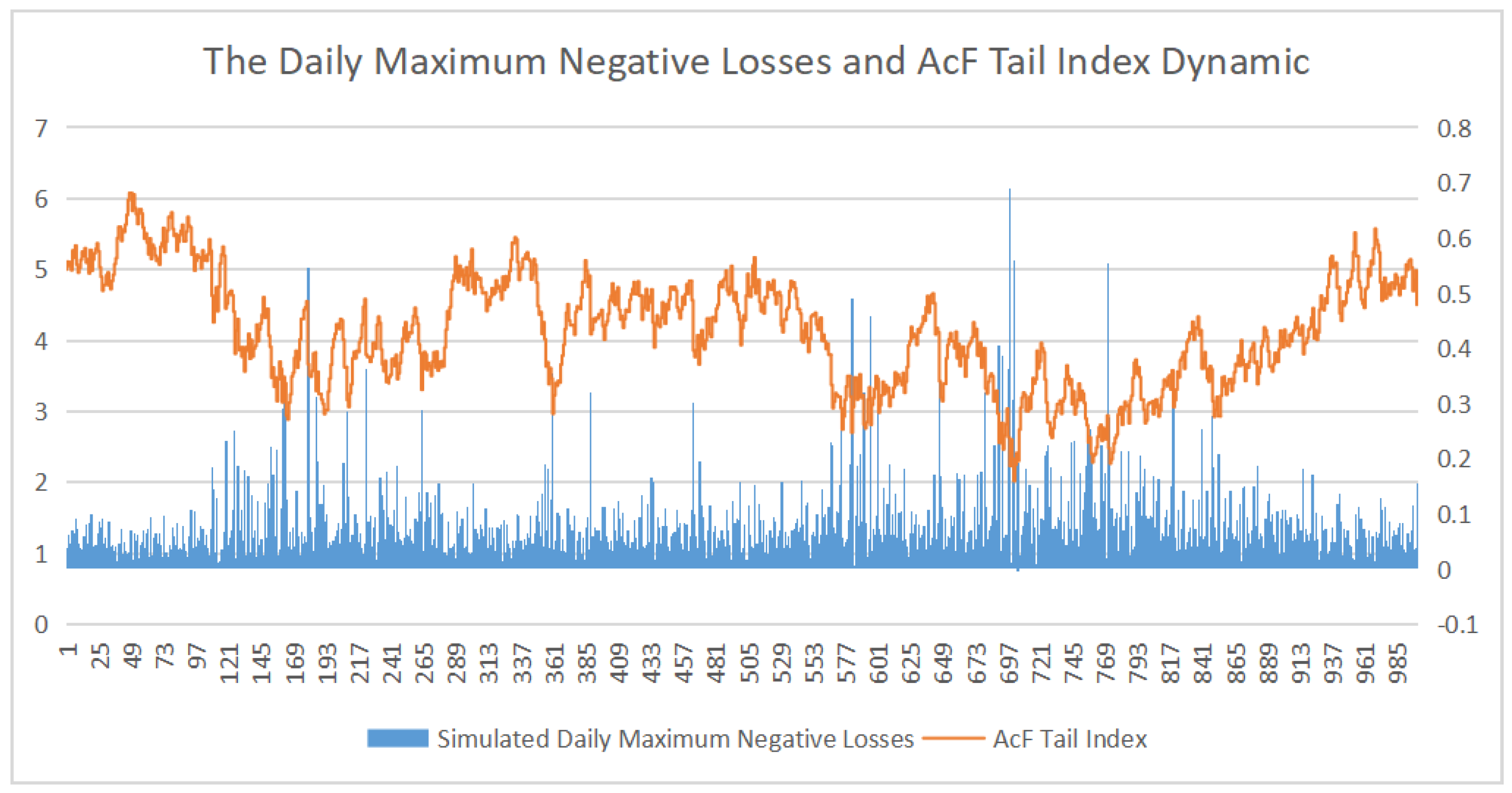
The dynamic Fréchet process, or the Autoregressive Conditional Fréchet (AcF) model is proposed by Zhao et al.(2018) [1]. Specifically, the AcF(1,1) model is utilized to describe and generate the “prices“ of the ad hoc “assets“ in this paper, which is expressed as follows:

$$Q_t=\mu +{\sigma }_t{Y}_t^{\frac{1}{\alpha {}_t}},$$

(3)

$$log{\sigma }_t={\beta }_0+{\beta }_{1}log{\sigma }_{t-1}+{\beta }_{2}exp(-{\beta }_3{Q}_{t-1}),$$

(4)

$$log{\alpha }_t={\gamma }_0+{\gamma }_{1}log{\alpha }_{t-1}+{\gamma }_{2}exp(-{\gamma }_3{Q}_{t-1}),$$

(5)

where $Y_t$ is a sequence of i.i.d. unit Fréchet random variables ($\mu =0,\sigma =1,\alpha =1$) with the distribution function $F\left(x\right)=e^{-1/x},x>0$, $0\le {\beta }_1\ne {\gamma }_1<1,{\beta }_2<0,{\beta }_3>0,{\gamma }_2>0$ and ${\gamma }_3>0$.

The parameters of AcF(1,1) model are of financial interpretability. $\mu$ is the location parameter that governs the overall location of $\left\{Q_t\right\}$ sequence. $\left\{{\sigma }_t\right\}$ is the dynamic Fréchet scale parameter which can be regarded as the dynamic volatility sequence. $\left\{{\alpha }_t\right\}$ is the dynamic Fréchet shape parameter, which measures the asymmetry of underlying “prices“ sequence $\left\{Q_t\right\}$. Using the AcF(1,1) model, one can generate $\left\{Q_t\right\}$ sequences for simulation studies (See Section 8) and other research purposes.

4. The Construction of Tail Risk Options

4.1. The Market Conventions

Issuance and expiration: A tail risk option (TRO) is written on the “value“ of tail risk, i.e., the “price“ of an ad hoc “asset“ proposed in Section 3 in a single given day (the “observation day,“ which will be introduced in the next sub-point). Thus, each TRO should be issued at any moment before that day, with a given “strike price“ K, which is a pre-determined value regarding the tail risk in the “observation day.“ The expiration time of a TRO is the closing time of its “observation day.“ The TRO can be issued and traded in the market or over-the-counter (OTC).

The “observation day“: An “observation day“ of a TRO is the date that the payoff of this TRO is calculated. Since the payoff of a TRO is computed using a whole day’s trading information on that day (see Section 4.2 for details), this option will be “observed“ all that day. This is the reason why this day is termed “observation day.“ Normally, the “observation day“ of a TRO is the final trading date, i.e., its maturity date.

4.2. The Payoffs

Similar to conventional options, there are two types of TRO in terms of the right and obligation of traders: call option, and put option. The TRO calls are options that the buyers expect higher “prices“ of the underlying “assets,“ that is, higher tail risks. When an observed value of tail risk (the ad hoc underlying “price“) is larger than a given one (the strike price), the payoff of a TRO call is positive; thus, the seller pays to the buyer. A similar situation applies to TRO puts.

Following Section 3.1, the payoff functions of a European TRO call and put are given by:

$$max(Q_{0,T}-K,0)$$

(6)

and

$$max(K-Q_{0,T},0),$$

(7)

respectively. K is the strike price. $Q_{0,T}$ is the “observed price“ of the ad hoc underlying asset at the “observation day“, and it can be either $Q_{t,T}^{HF}$ or $Q_{t,T}^{HD}$. Written on different underlying “assets,“ the TROs can be further refined to other kinds of options regarding their payoff.

Type I TRO: high-frequency index option. If $Q_{0,T}$ is defined by Equation (1), i.e., the TRO is written on Type I ad hoc “asset“, thereby, the TRO can be refined as a high-frequency index option with payoff functions:

$$max\left\{max(X_{1,0,T},X_{2,0,T},\cdots ,X_{M-1,0,T},X_{M,0,T})-K,0\right\}$$

(8)

for calls, and

$$max\left\{K-max(X_{1,0,T},X_{2,0,T},\cdots ,X_{M-1,0,T},X_{M,0,T}),0\right\}$$

(9)

for puts. It is natural to choose an index instead of a single specific asset (a stock or a bond) as the underlying asset because the concept of tail risk refers to the entire market (systemic risks) rather than a specific asset (individual risks).

Type II TRO: high-dimensional rainbow option. If $Q_{0,T}$ is defined by Equation (2), i.e., the TRO is written on Type II ad hoc “asset“, thereby, the TRO can be refined as a high-dimensional rainbow option written on N assets with payoff functions:

$$max\left\{max(L_{1,t,T},L_{2,t,T},\cdots ,L_{N-1,t,T},L_{N,t,T})-K,0\right\}$$

(10)

for calls, and

$$max\left\{K-max(L_{1,t,T},L_{2,t,T},\cdots ,L_{N-1,t,T},L_{N,t,T}),0\right\}$$

(11)

for puts.

Ideally, in practice, the high-frequency traders can utilize Type I TRO to hedge tail risks in the time series level, such as to avoid the extreme losses caused by maximum drawdowns; and the portfolio managers can use Type II TRO to hedge tail risks in the cross-sectional level, such as to avoid the extreme losses caused by every single asset within her portfolio (see Section 9.3 for more discussion regarding the implications). In addition, if the newly designed TROs are traded in markets and have sufficient liquidity, they can signal the market sentiments towards financial crises for both investors and policy-makers. This application will be illustrated using a simulated example in Section 8.

5. The Closed-Form Pricing Formulas for TROs

By assuming $Q_{0,T}$ follows the Fréchet distribution $F\left(x\right)=e^{-{\left(\frac{x-\mu }{\sigma }\right)}^{-\alpha }},x>0$, and $\mu$, $\sigma$, and $\alpha$ are location, scale, and shape parameters, respectively. We obtain the analytical valuation formulas for the newly designed TROs as:

$$C_t\left(K\right)=e^{-r(T-t)}\sigma ·\Gamma (1-\frac{1}{\alpha },H^{-\alpha })-(K-\mu )e^{-r(T-t)}·[1-e^{-H^{-\alpha }}],(\alpha >1)$$

(12)

for calls, and

$$P_t\left(K\right)=(K-\mu )e^{-r(T-t)}·e^{-H^{-\alpha }}-e^{-r(T-t)}\sigma ·{\Gamma }^U(1-\frac{1}{\alpha },H^{-\alpha }),(\alpha >1)$$

(13)

for puts, where r is the risk-free rate, $H=(K-\mu )/\sigma$, $\Gamma (·,·)$ is the lower incomplete gamma function, and ${\Gamma }^U(·,·)$ is the upper incomplete gamma function. t can be any time before the expiration time T.

The condition $\alpha >1$ in Equations (12) and (13) is to guarantee that the inputs of the incomplete gamma function are nonnegative. (See Appendix A for details.) According to Hansen (1994) and Zhao et al. (2018) [1,33], this condition is almost surely satisfied because $\alpha$ is usually larger than 4 in real data. According to Hansen (1994) [33], when $\alpha$ is lower than 2, the second moment does not exist. For details of derivations for calls, see Appendix A. The derivation of TRO put prices is analogous to that of calls and is, hence, omitted.

The resulting pricing formulas are of great simplicity and interpretability. Both Equations (12) and (13) involve only three parameters of the Fréchet distribution: $\mu$, $\sigma$, and $\alpha$. Thus, trading the TROs is essentially trading the investors’ views about these three underlying parameters in the future. The location parameter $\mu$ reflects the “worst“ situation for the maximum loss. If the TRO is used for portfolio tail risk hedging (that is, the Type II TRO), $\mu$ can be seen as the minimum return that all assets in the portfolio are rising simultaneously. Thus, the condition $Q_{0,T}>\mu$ must hold in real data. The scale parameter $\sigma$ is analogous to the B-S implied volatility, a model-based volatility measure. The shape parameter $\alpha$ is the only parameter that governs the asymmetry and how “fat“ is the tail. Theoretically, the smaller the $\alpha$, the more severe asymmetry of the underlying distribution, and the higher the tail risk (Jang and Krvavych, 2004; Shrivastava et al., 2011; Zhao et al., 2018) [1,4,5]. See Section 7 for simulation results that show how the TROs prices change with $\sigma$ and $\alpha$.

6. Simulation Study: Pricing Performance of the TRO Pricing Formulas

In this section, Monte Carlo experiments are conducted to investigate the pricing performance of the pricing Equations (12) and (13). (There are necessities for examining the pricing accuracy of the proposed pricing formulas. First, pricing is a natural and must-do work for a newly proposed financial product. In this sense, a rational market equilibrium does not admit arbitrage or much pricing bias. Second, we obtain a closed-form solution for TROs prices by considering asymmetric features of extreme losses and tail risks and using extreme value theory, which serves as one of the novelties of this paper. We need to demonstrate that the novel result is trustworthy. Finally, one of the applications of TROs is to measure market sentiments toward tail risks and financial crises. To do this, an explicit formula for TRO price has to be given, with one or more parameter(s) clearly and precisely corresponding to different types of risks. See Section 8 for this issue.) We simulate TRO prices by generating Fréchet random variables with the location parameter $\mu =0$, the scale parameter $\sigma =0.135$, and the shape parameter $\alpha =3,4,5,6,$ and 7. We choose $\mu =0$ because the location parameter is close to 0 in real data (Zhao et al., 2018) [1]. The choice of scale parameter is base on the mean of the estimated typical range ([0.06, 0.21]) of the AcF scale parameter for $S\&P100$ portfolio (Zhao et al., 2018) [1]. Simulations are conducted 100,000 times separately for each tail index value. To illustrate the method, we select $r=0.03$, consistent with recent history. K ranges from 0.01 to 0.80 by step size 0.01. $T-t=1$ (day) corresponds to the fact that there is only one day of “observation“ for each TRO. The main results may not change when the time to maturity is set to be other values. The Monte Carlo TRO prices are computed by

$$C^{MC}=e^{-r(T-t)}max(Q_{0,T}-K,0)$$

(14)

for calls, and

$$P^{MC}=e^{-r(T-t)}max(K-Q_{0,T},0)$$

(15)

for puts.

The root mean squared error (RMSE) and maximum absolute error (MAE) are computed via (16) and (17), and are shown in

Table 1. Pricing performance in terms of RMSE and MAE.

	RMSEcall	RMSEput	MAEcall	MAEput
$\alpha =3$	$1.7539\times {10}^{-4}$	$4.5043\times {10}^{-5}$	$4.3008\times {10}^{-5}$	$1.4291\times {10}^{-5}$
$\alpha =4$	$5.6705\times {10}^{-5}$	$2.4401\times {10}^{-5}$	$1.6823\times {10}^{-5}$	$7.8508\times {10}^{-6}$
$\alpha =5$	$1.3918\times {10}^{-5}$	$7.2705\times {10}^{-6}$	$7.2705\times {10}^{-6}$	$3.5977\times {10}^{-6}$
$\alpha =6$	$1.6123\times {10}^{-5}$	$1.0564\times {10}^{-5}$	$6.5398\times {10}^{-6}$	$3.0115\times {10}^{-6}$
$\alpha =7$	$9.3093\times {10}^{-6}$	$7.6468\times {10}^{-6}$	$4.3364\times {10}^{-6}$	$3.4457\times {10}^{-6}$
average	$5.6358\times {10}^{-5}$	$2.0314\times {10}^{-5}$	$1.5595\times {10}^{-5}$	$6.4393\times {10}^{-6}$

.

$$RMSE\left(t\right)=\sqrt{\frac{{\sum }_N{[Pric{e}^{Model}-Pric{e}^{MC}]}^2}{N}},$$

(16)

$$MAE\left(t\right)=\sqrt{\frac{{max}_N|Pric{e}^{Model}-Pric{e}^{MC}|}{N}},$$

(17)

where $Pric{e}^{Model}$ stands for TRO calls or puts prices computed by pricing models (12) and (13), $Pric{e}^{MC}$ stands for M.C. prices computed by (14) and (15), and N is the sample size.

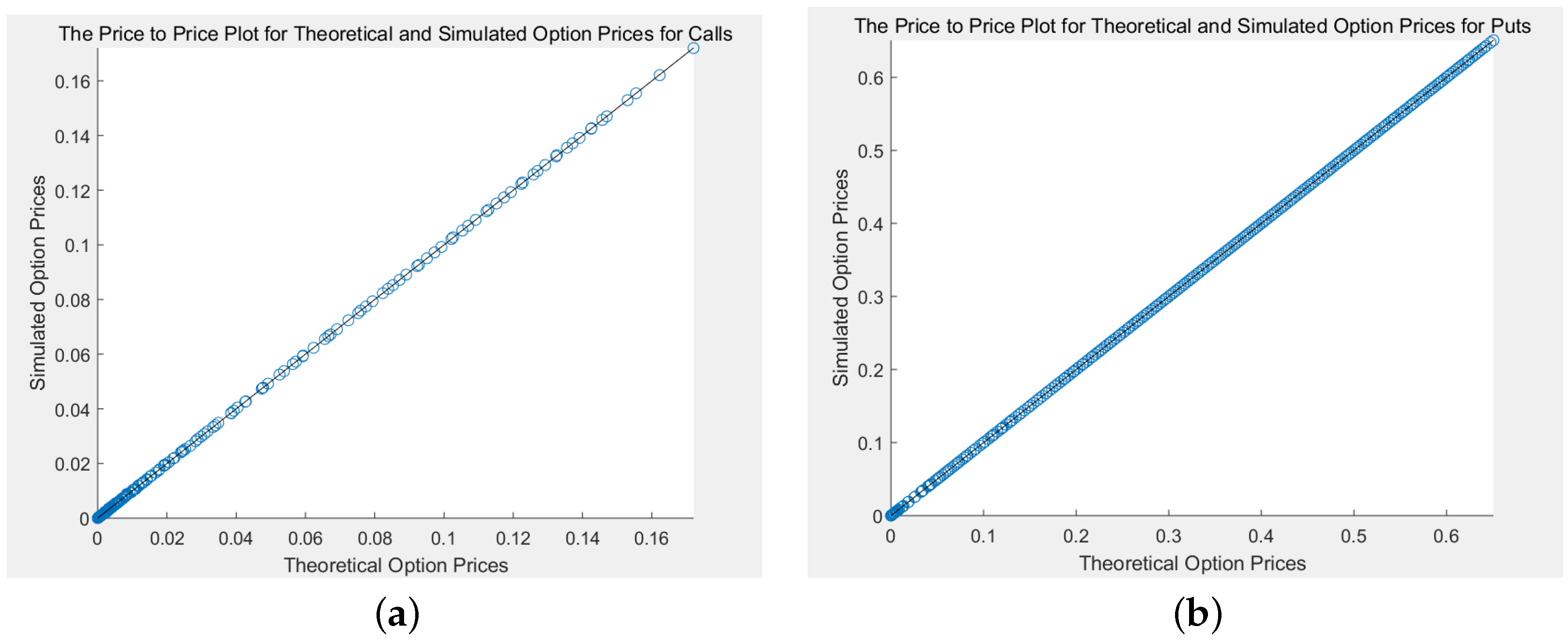
The price-price plots (pp-plots, theoretical prices in the x-axis, simulated prices in the y-axis) are shown in Figure 1.

In Table 1, the average RMSE is $5.6358\times {10}^{-5}$ for calls and is $2.0314\times {10}^{-5}$ for puts. The average MAE is $1.5595\times {10}^{-5}$ for calls and is $6.4393\times {10}^{-6}$ for puts. The RMSE and MAE for each case are no more than $1.7539\times {10}^{-4}$ and $4.3008\times {10}^{-5}$, respectively. In Figure 1, almost all the points lie on the line of ${45}^{\circ }$. The above results have shown the pricing accuracy of the proposed pricing models.

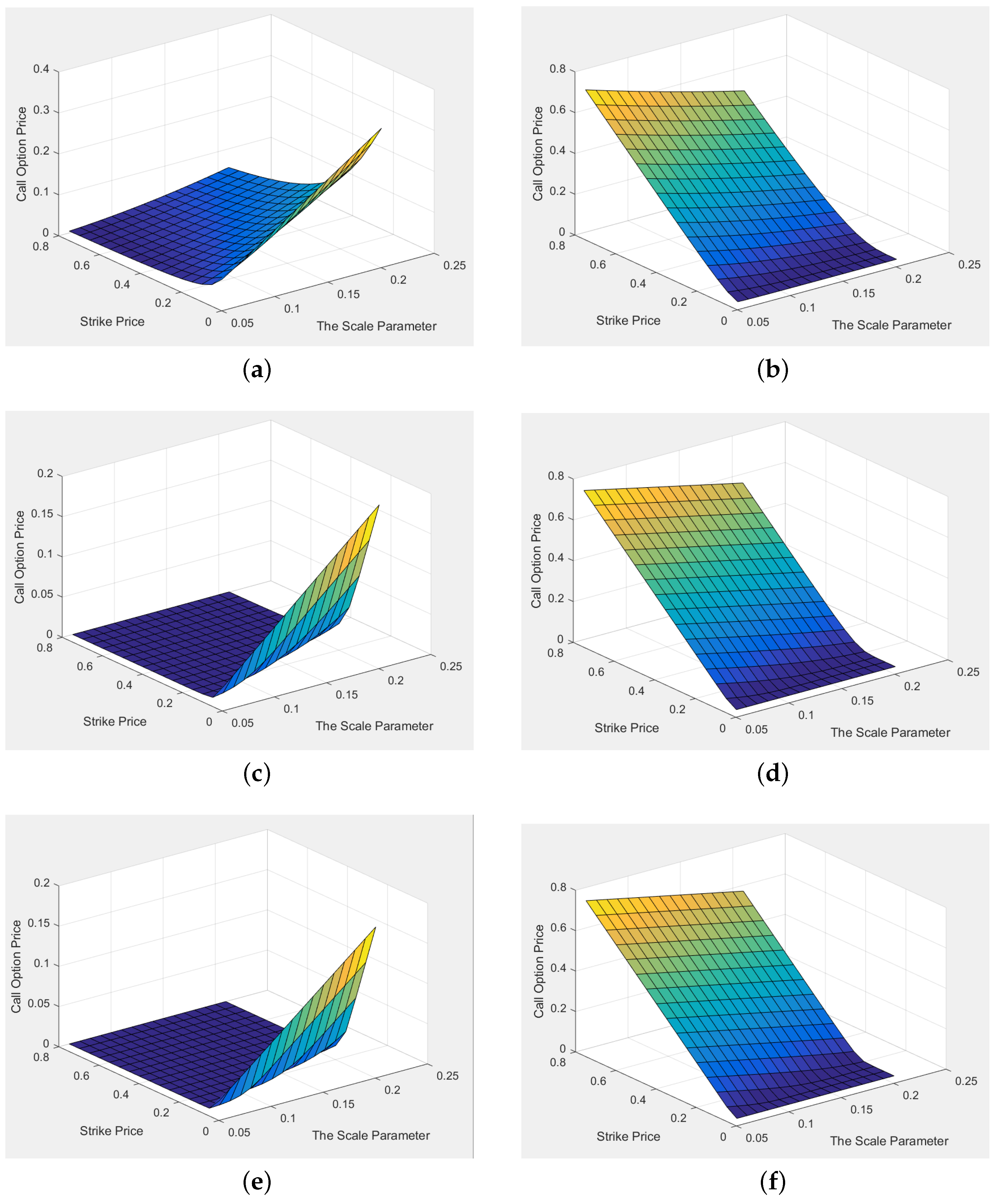
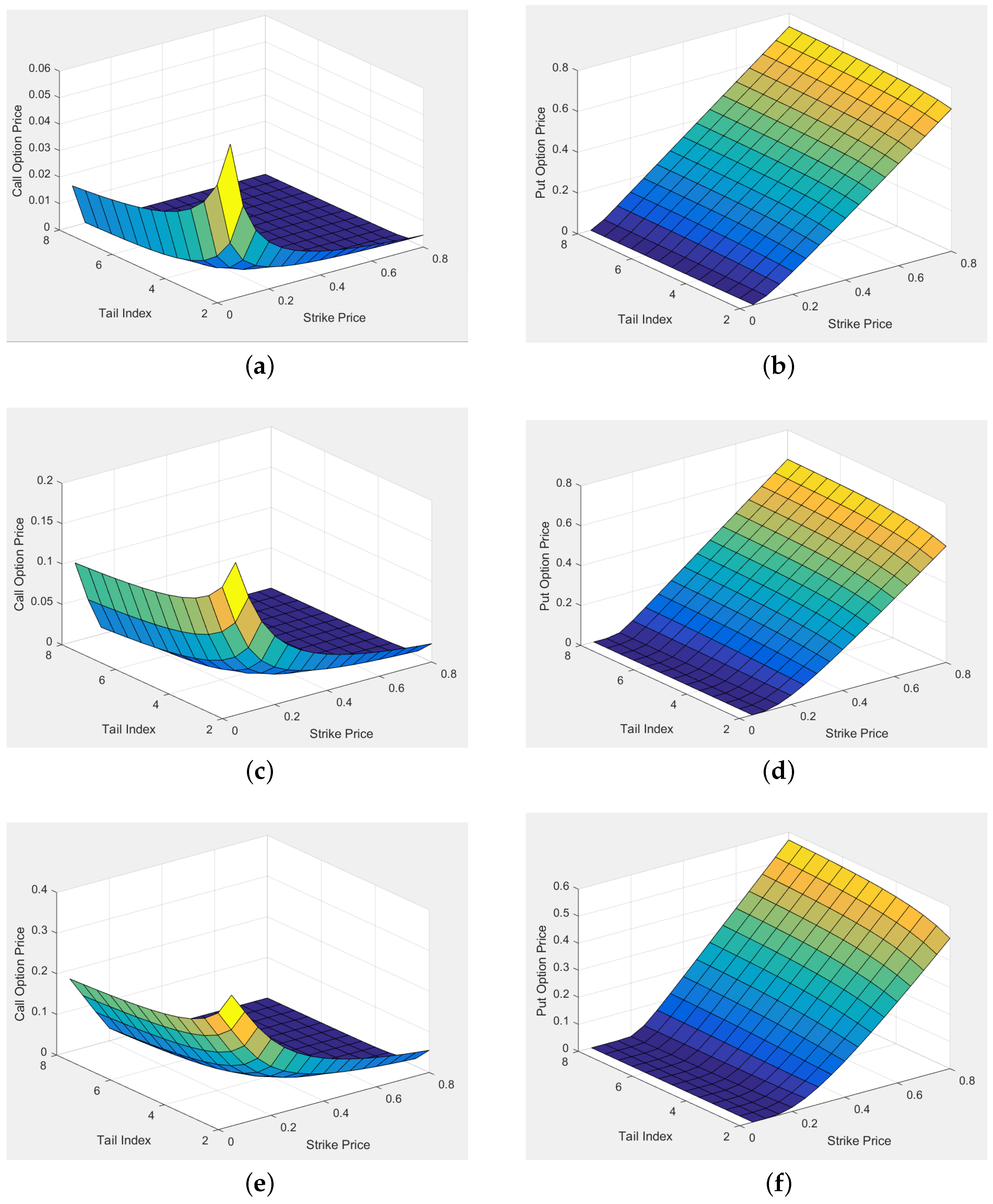
7. Simulation Study: TRO Price, Volatility, and Tail Index

The newly designed TRO can be used to evaluate both “normal“ (symmetric) risk and tail (asymmetric) risk, where the “normal“ risk represents how the market fluctuates when skewness and kurtosis remain unchanged, and the tail risk represents the occurrence of a market crash and financial crisis. To demonstrate this fact, Monte Carlo simulations are conducted to investigate how the TRO prices change with $\sigma$ and $\alpha$. According to the empirical results of $S\&P100$ (Zhao et al., 2018) [1], the typical range of $\sigma$ and $\alpha$ are [0.06, 0.21] and [2, 8], respectively. Based on these results, we set $\sigma$ from 0.06 to 0.21 by step size 0.01, and set $\alpha$ from 2 to 8 by step size 0.5. When examining how option price changes with the $\alpha$, we set volatility $\sigma$ at three different levels: high ($\sigma =0.21$), medium ($\sigma =\frac{1}{2}·0.21+\frac{1}{2}·0.06=0.135$), and low ($\sigma =0.06$). When examining how option price changes with $\sigma$, we set $\alpha$ at three different levels: high ($\alpha =2$), medium ($\sigma =\frac{1}{2}·2+\frac{1}{2}·8=5$), and low ($\alpha =8$). Each scenario is conducted for different K ranging from 0.05 to 0.80 by step size 0.05. For consistency, $\mu$, and r are set to be the same as in the previous section. The results for TRO calls and puts are shown in Figure 2 and Figure 3, respectively.

In Figure 2, for each K, the lower the tail index $\alpha$ (meaning a higher tail risk), the higher the price of the TRO calls, and the lower the price of the TRO puts. This conclusion holds for all TROs at different volatility levels, which shows the robustness of our conclusion.

The underlying logic of the above results is that a smaller tail index value means greater asymmetry in the distribution of the ad hoc “asset“ and, thus, a larger tail risk. Consequently, the demand for TRO calls increases, and their prices go up, whereas the demand for TRO puts decreases, and they become cheaper.

Meanwhile, the overall level of volatility determines the overall level of TRO price surface. By comparing Figure 2a,c,e, one can find that the greater the volatility, the higher the price of the TRO calls (for the same K). Conversely, by comparing Figure 2b,d,f, we find that the greater the volatility, the lower the price of the TRO puts (for the same K).

The relationship between the TRO price and volatility is similar to that of tail index. According to Figure 3, for each K, when $\sigma$ increases, the TRO call prices go up, and the put prices go down. This conclusion holds for different $\alpha$, which shows the robustness of the conclusion. By comparing Figure 3a,c,e, we find that the higher the tail risk (smaller value in $\alpha$), the more expensive the TRO calls. By comparing Figure 3b,d,f, we find that the higher the tail risk, the cheaper the puts.

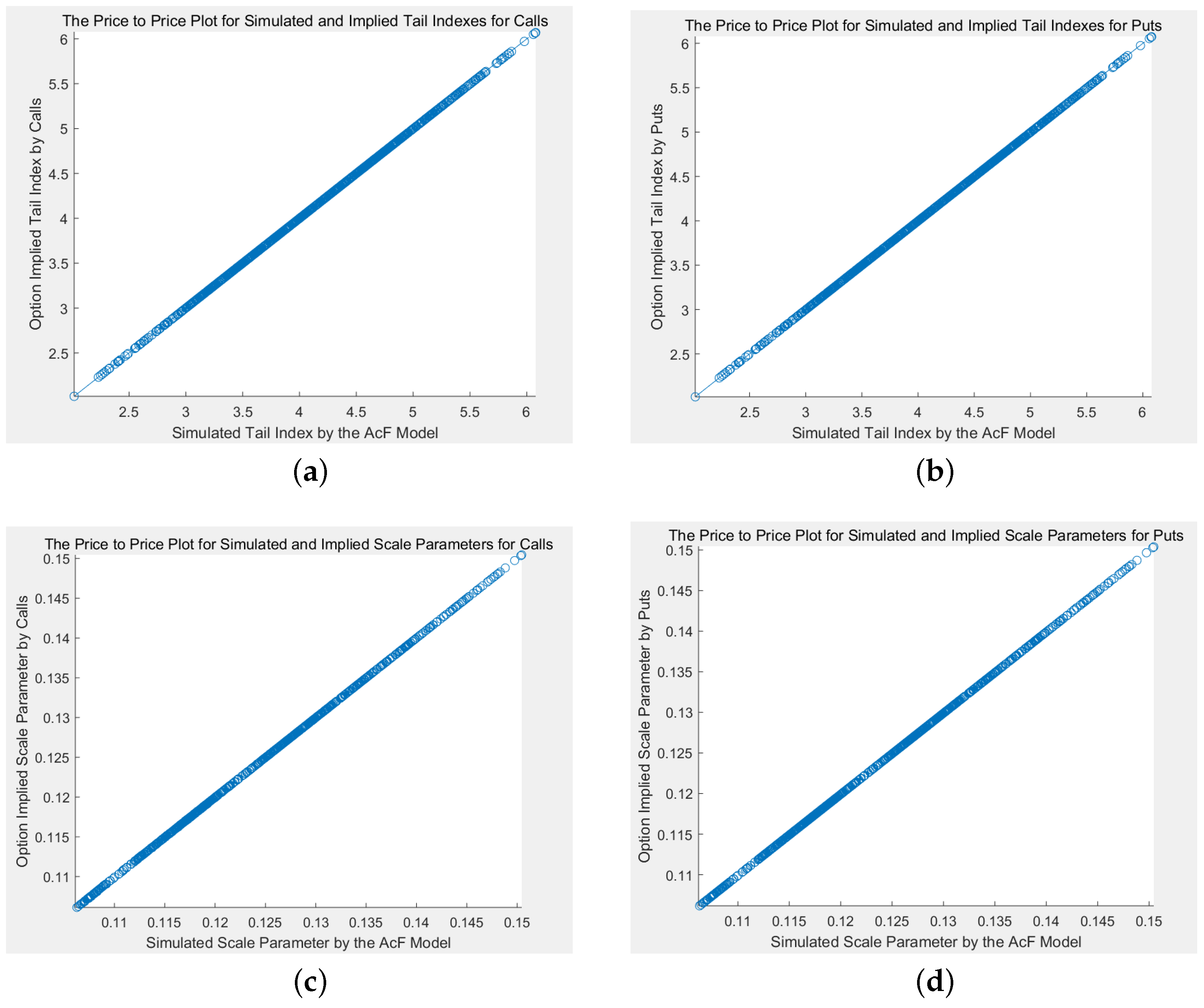
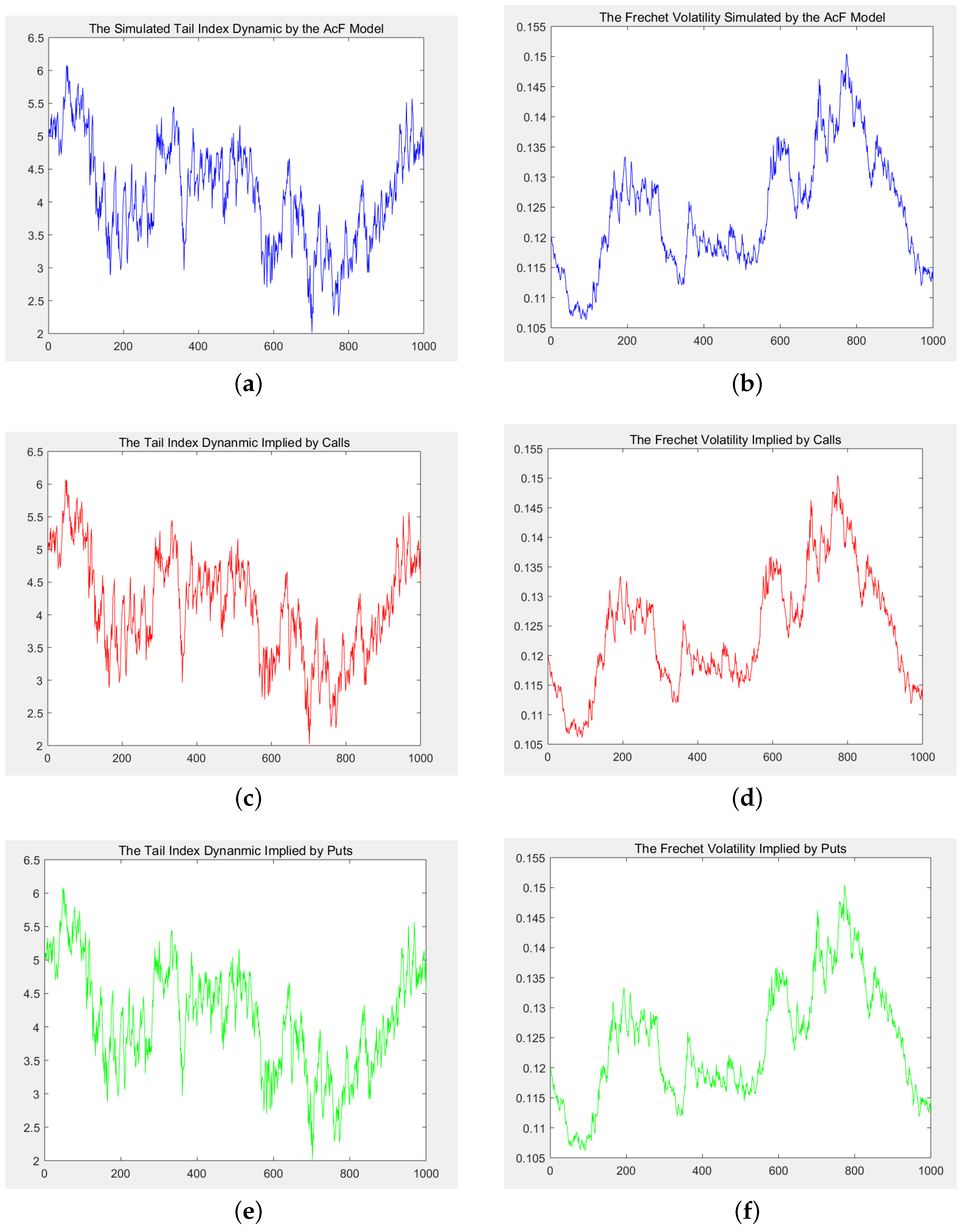
To sum up, no matter whether at scale level (“normal“ risk, with greater volatility $\sigma$) or at shape level (tail risk, with a smaller value in tail index $\alpha$), the greater the risk, the more expensive the TRO calls, and the cheaper the TRO puts. Since the TRO prices depend on the market’s view on both “normal“ risk and tail risks, the prices can be natural evaluations of these market risks. To simultaneously imply these two risks from the TRO price, one can use the probability method for calibration, introduced in Section 8.1.

8. Application: Implying the Tail Risks from TRO Prices

There are two ways to understand market views. One is through the model, and the other is through the option price. When we are calibrating an option pricing model, we learn the market views and the market sentiments. This section provides a model-based method and simulated example to demonstrate how the market sentiments towards symmetric risk (volatility) and asymmetric risk (tail risk) are implied by TROs prices. The resulting implied TRO-volatility and TRO-tail risk index correspond to symmetric and asymmetric risks, respectively.

8.1. Methodology

In reality, one can use the probability method to calibrate the TRO pricing models (12) and (13) for inferring the market views on (tail) risks. The calibration can be fulfilled by minimizing the sum of squared errors (SSE) between theoretical and real TRO prices with the following objective functions:

$$\underset{{\theta }_t}{min}SS{E}_t^{Call}=\underset{{\theta }_t}{min}\sum _K{[C_t\left(K\right)-\widehat{C_t}\left(K\right)]}^2,\forall t,$$

(18)

$$\underset{{\theta }_t}{min}SS{E}_t^{Put}=\underset{{\theta }_t}{min}\sum _K{[P_t\left(K\right)-\widehat{P_t}\left(K\right)]}^2,\forall t,$$

(19)

where the subscript t stands for the t-th trading day, ${\theta }_t$ represents the risk-neutral parameters of the pricing models in day t, i.e., ${\theta }_t=({\mu }_t,{\sigma }_t,{\alpha }_t)$. Calibrating the model every trading day, and the implied Fréchet volatility dynamic $\left\{\widehat{{\sigma }_t}\right\}$ and the implied tail index dynamic $\left\{\widehat{{\alpha }_t}\right\}$ can be obtained.

8.2. Simulation Example

In this subsection, we demonstrate how the symmetric and asymmetric risks are decomposed and, thereby, how the market tail risks can be implied by TROs prices using the calibration procedure given in Section 8.1. In addition, the example explains how the implied tail index acts as a measure of market sentiment and tail risk. Since the newly introduced TRO does not yet exist in the market, we provide the following example using simulated data. However, it is hopeful that, if the newly designed TRO starts trading in the market, the following work can be finished with real data.

To simulate the changing scenario, we firstly generate TRO prices from Equations (12) and (13) with time-varying parameters given by the AcF(1,1) models (3)–(5), and then calibrate the TRO pricing models via Equations (18) and (19).

To study the dynamics of tail indexes, we consider TROs that are continually issued (and re-issued) for 1000 days (about 4 years, suppose about 250 trading days per year). Parameters r and K are set the same as in previous sections. The AcF(1.1) parameters values are chosen according to the empirical results of $S\&P100$ portfolio (Zhao et al., 2018) [1], that is,

$$[{\beta }_0,{\beta }_1,{\beta }_2,{\beta }_3,{\gamma }_0,{\gamma }_1,{\gamma }_2,{\gamma }_3,\mu ]=[-0.050,0.961,-0.051,6.68,-0.068,0.89,0.328,5.33,-0.069].$$

The reason why this paper utilizes these estimated results is to keep consistent with the most recent results, so that the simulation example conducted in this section can provide a good mimic for reality. (Since the newly proposed TROs have not yet been traded in markets, it is impossible to provide a real data-based example here. Nevertheless, once the TROs start trading, one can calibrate the underlying AcF model and obtain specific resulting parameters for different markets in a different time span.)

The simulated AcF tail index $\left\{{\alpha }_t\right\}$ and corresponding $\left\{Q_t\right\}$ are displayed in Figure 4. The p-p plots for calibrated and simulated parameters are shown in Figure 5. The implied volatility dynamic $\left\{\widehat{{\sigma }_t}\right\}$, implied tail index dynamic $\left\{\widehat{{\alpha }_t}\right\}$, and their corresponding “ture values“ (the simulated values) are shown in Figure 6.

As shown in Figure 4, the AcF tail index goes negatively correlated with $\left\{Q_t\right\}$. When $\left\{Q_t\right\}$ is unusually large (close to 0.8), the tail index value is close to 2, which is the threshold for the existence of the second moment (Hansen, 1994) [33]. The p-p plots in Figure 5 show the accuracy of calibration, which indicates that the methodology of calibration is applicable and practical.

Comparing the TRO-implied tail indexes with the AcF $\left\{{\alpha }_t\right\}$ in Figure 6, it is shown that the trends of TRO implied tail indexes and the AcF $\left\{{\alpha }_t\right\}$ are almost the same. When the AcF tail index reaches its lowest point (about 2, meaning a crisis), the implied tail indexes for both call and put also go down to about 2. The above finding means that the TRO-implied tail indexes can be mirrors of market sentiment and crisis warning. A relatively lower implied tail index implies a relatively larger asymmetry of the underlying distribution for losses and a more severe fear of investors for the upcoming crisis.

Similar findings can also be seen in the TRO-implied volatility $\left\{\widehat{{\sigma }_t}\right\}$. In Figure 6, the implied $\left\{\widehat{{\sigma }_t}\right\}$ for both calls and puts share the same pattern with the AcF $\left\{{\sigma }_t\right\}$, which means the calibration for the scale parameter is also “correct.“ The basic financial interpretation for $\left\{\widehat{{\sigma }_t}\right\}$ is similar to the Black-Scholes implied volatility, which is a measure for the overall “normal“ risk.

9. Conclusions, Implications, and Future Research Directions

9.1. Conclusions

Tail risk hedging is an important issue for both investors and policy-makers. However, directly hedging tail risks with an ad hoc option is still an unresolved problem in existing literature because of the asymmetric features of losses and tail risks. Ignoring the asymmetric nature of tail risks may cause mis-specification for the pricing kernel and, thereby, jeopardize option pricing accuracy, and even the existence of closed-form solutions for option prices.

This paper defines two ad hoc underlying “assets“ and designs two novel tail risk options (TROs) for hedging and evaluating short-term tail risks to fill the existing gaps. The newly designed TRO can be written on either the daily maximum negative loss of a basket of the underlying portfolio or the maximum daily high-frequency negative loss of an underlying index. Furthermore, by assuming the underlying losses theoretically follow the Fréchet distribution, the closed-form pricing formulas for TRO European calls and puts are obtained. In addition, besides contract parameters, the resulting analytical pricing formulas involve only three parameters of the underlying distributions: the location parameter $\mu$, scale parameter $\sigma$, and shape parameter $\alpha$, each of them is of great interpretability.

The Monte Carlo simulation shows the pricing accuracy of the proposed pricing models and the fact that both the signals of symmetric (“normal“) risks and asymmetric (tail) risks can be detected from TRO prices. For example, when the market volatility goes up, the TRO calls become more expensive, the TRO puts cheaper, and vice versa. Conversely, when the tail index goes down (indicating a higher tail risk), the prices of TRO calls go up, and the prices of TRO puts go down. Therefore, in a financial sense, trading the newly designed TRO is essentially trading investors’ different attitudes towards both symmetric and asymmetric risks.

Using calibration, symmetric risk (volatility) and asymmetric risk (tail risk) components can be implied and decomposed from TRO prices. The TRO-implied volatility is analogous to the Black-Scholes implied volatility, which can measure the overall market volatility. The TRO-implied tail index can be a mirror of market sentiment and crisis warning. A relatively low tail index value implies a greater asymmetry in the underlying loss distribution and reflects greater panic and anxiety among market investors about the crisis.

9.2. Implications for Practice

The newly proposed TRO provides significant implications for investors, portfolio managers, and policy-makers.

First, investors and speculators can “bet on“ tail risks by trading TROs. For speculators, especially those have clear market views towards tail events, the newly designed TRO is an ideal financial instrument to “trade“ their opinions regarding tail risks. If they believe an upcoming extreme event (for example, a sudden natural disaster, such as the 2021 flood in central China area, or a public health event, such as COVID-2019) may cause a huge loss on assets, that is, they take “bullish“ attitudes towards tail risk, the “speculators“ can simply long TRO calls or short TRO puts. On the contrary, if the investors are optimistic about the markets, that is, they are “bearish“ on tail risk, they may short TRO calls or long TRO puts. After “gambling“ in either side, the speculators would keep only one single side in their positions until expiration. This is analogous to the “buy and hold“ strategy in trading conventional options. Without TRO, it is not easy to use the conventional option for tail risk betting.

Second, high-frequency traders and portfolio managers may optimize their tail risk management problem using TROs. As reviewed in Section 2, tail risk can be found in two dimensions: the time series level and cross-sectional level. In practice, the time series tail risk provokes the high-frequency traders, whose goal is to minimize their maximum drawdown; while the cross-sectional tail risk is usually considered by portfolio managers, whose objective is to avoid the worst scenario for each individual asset within her portfolio. Regarding these two purposes, the newly proposed TRO provides a direct tail risk hedging methodology, as the underlying “assets“ of TRO are no more but the “prices“ of these two kinds of tail risks they are facing. Thus, comparing with strategy-based (indirect) hedging, hedging tail risks with TRO provides a more straightforward way for risk managers to avoid extreme losses.

Third, policy-makers can adapt and adjust policies (especially monetary policy) for providing market liquidity by learning the market view towards tail risks via the TRO-implied tail indexes. Extreme losses in the capital markets call for monetary policy reaction to reduce market turbulence, and central bank asset purchases can provide insurance against tail events (Brunnermeier et al., 2014) [34]. Meanwhile, unconventional monetary policy (UMP) announcements can substantially reduce equity market tail risks and interest rate risks (Hattori et al., 2016) [35]. However, the nodus in these announcements is that the central banks need to predict changes in market sentiment and provide sufficient liquidity through open market operations before the possible tail risks and liquidity crises occur. Regarding this point, the TRO-implied tail risk index is an ideal tool for central banks and policy-makers to detect market views and sentiments. In practice, an extreme low value in TRO-implied tail index means an urgent warning for upcoming “tight“ market liquidity, and the policy-makers may react in advance by using UMP or directly purchase assets via open market operations.

Given the above implications, we argue that there are novelties of the TRO-based tail risk hedging methodology adding to conventional tail risk hedging methods. First, compared with the indirect hedging philosophy proposed by Bhansali (2014) [2], trading TRO is much more straightforward for traders and portfolio managers to hedge tail risks. Second, the conventional indirect hedging method, which is a trading strategy-based methodology, works mainly for long-term risks. When it comes to the extreme losses in a very short time period, direct hedging using TRO can be relatively more efficient and effective. Third, from a macroeconomic perspective, conventional methods provide with very little information to policy-makers, while the TRO-implied tail risk index can be a measure of the systemic risk regarding the entire market and, thereby, contribute to market risk management at a macro level.

9.3. Limitations and Future Study Directions

There are limitations of this research, which are mainly because of the lack of real TRO price data. The following gaps can be filled once the real data released and, thus, are left as further empirical research directions.

First, the application example in this paper is based upon simulated data rather than real data, as the newly proposed TRO has not yet being traded in the market. Empirically, it is interesting to ask whether the newly proposed TRO can reduce the losses cased by extreme events and, thus, improve market efficiency.

Second, the TRO pricing formula proposed in this paper is a static pricing model, rather than a dynamic one. In the future, it will be interesting and meaningful to generate the pricing model into the one with time-varying parameters. Moreover, since the way to extend the model is not unique, one can select a best-fitted model or a best-interpreted model among several competing models using real data in the future.

Third, this paper mainly focus on the design, pricing, and application issues of TRO. Based on that, trading and hedging strategies regarding TRO can be further discussed. In practice, the TRO-related risk exposure for sellers can be extremely large, which stresses the necessity of reasonable inventory management rules and hedging methods. Regarding this issue, novel Greeks for the Fréchet can be developed. Comparing to B-S Greeks which are linked with many (normal) risk factors, the TRO-based Greeks reflect the sensitivities between: (1) the TRO price and the ad hoc “asset“ volatility $\sigma$; and (2) the TRO price and the tail index $\alpha$.