Experimental Design for the Lifetime Performance Index of Weibull Products Based on the Progressive Type I Interval Censored Sample

Abstract

In this study, the experimental design is developed based on the testing procedure for the lifetime performance index of products following Weibull lifetime distribution under progressive type I interval censoring. This research topic is related to asymmetrical probability distributions and applications across disciplines. The asymptotic distribution of the maximum likelihood estimator of the lifetime performance index is utilized to develop the testing procedure. In order to reach the given power level, the minimum sample size is determined and tabulated. In order to minimize the total cost that occurred under progressive type I interval censoring, the sampling design is investigated to determine the minimum number of inspection intervals and equal interval lengths when the termination time of experiment is fixed or not fixed. For illustrative aims, one practical example is given for the implementation of our proposed sampling design to collect the progressive type I interval censored sample so that the users can use this sample to test if the lifetime performance index exceeds the desired target level.

1. Introduction

For the larger-the-better-type quality characteristics like the lifetimes of products, the unilateral process capability index C_L proposed by Montgomery [1] is used to assess the performance of the lifetimes of products. This index is so-called the lifetime performance index. For a complete sample, Tong et al. [2] utilized the uniformly minimum variance unbiased estimator (UMVUE) of C_L to develop a testing computational algorithm for exponential products. In many cases, the experimenters can only observe censored data. Two censoring types, including type I censoring and type II censoring, are frequently considered. Type I censoring occurs if the life test of n subjects stops at a predetermined time and the number of observations is random. Type II censoring occurs if the life test stops when a predetermined number of failure times are observed. Progressive censoring has the property of allowing the removal of units at some time points that may not be the final termination point. Referring to Yadav et al. [3], Jäntschi et al. [4], Chen and Gui [5], Balakrishnan and Aggarwala [6] and Aggarwala [7], we can see more inferences about the progressive censored data. For progressive type II censored data, Lee et al. [8] constructed a testing procedure for the lifetime performance index. We referred to Wu et al. [9] and Wu et al. [10] for step–stress accelerated life testing data. For this type of censored data, the lifetime performance index of exponential products was evaluated by Lee et al. [11]. For progressive type I interval censored data, a testing procedure for the lifetime performance index was assessed by Wu and Lin [12] using the maximum likelihood estimator as the testing statistic for exponential products. For products following the Gompertz lifetime distribution, a testing procedure for the lifetime performance index was proposed by Wu and Hsieh [13] based on a progressive type I interval censored sample. Based on this testing procedure, a reliability sampling design was developed by Wu et al. [14] for products following Gompertz distribution. For products following Weibull lifetime distribution, Wu and Lin [15] proposed a hypothesis testing procedure for the lifetime performance index using progressive type I interval censored data, and the proposed testing procedure is summarized in Section 2. The conforming rate is defined as the probability that the product life exceeds the given lower specification limit. It is an increasing function of the lifetime performance index. By this monotonic relationship, the experimenters can determine the desired target value for the lifetime performance index so that the conforming rate can be sustained. Based on progressive type I interval censored data, the testing procedure to see if the lifetime performance index meets the desired target value is proposed. The research goal of this paper is to develop a sampling design under three cases for the testing procedure proposed in Wu and Lin [15] using a progressive type I interval censored sample. The first case is to determine the sample size so that the preassigned test power can be attained for a level α test. The second case is to determine the number of inspection intervals so that the total experimental cost can be minimized when the termination time of the experiment is fixed. The third case is to determine the number of inspection intervals and inspection interval lengths by minimizing the total cost for the test on the evaluation of the lifetime performance index when the termination time is not fixed. The algorithms, figures and tables are shown in Section 3.1, Section 3.2 and Section 3.3. Our algorithms can help experimenters to set up a progressive type I interval censoring scheme. For the aim of illustration, one practical example is given to demonstrate the implementation of this sampling design to collect the progressive type I interval censored data, and then, the experimenters can use this data to test whether or not the process is capable. Our research results are only applicable for Weibull lifetime distribution, and the research results in Wu et al. [14] are only applicable for Gompertz lifetime distribution. Finally, the conclusion is made in Section 4.

2. The Introduction of the Testing Procedure for the Lifetime Performance Index in Wu and Lin

We consider that the lifetimes U of products follow a two-parameter Weibull distribution. The probability density function (pdf) and the cumulative distribution function (cdf) for U are given as follows:

$$f_U(u)=\frac{\delta }{\lambda }{(\frac{u}{\lambda })}^{\delta -1}\exp \left\{-{(\frac{u}{\lambda })}^{\delta }\right\},u>0,\delta >0,\lambda >0$$

(1)

and

$$F_U(u)=1-\exp \left\{-{(\frac{u}{\lambda })}^{\delta }\right\},u>0,\delta >0,\lambda >0,$$

(2)

where $\lambda$ is the scale parameter and $\delta$ is the shape parameter. The application of Weibull distribution refers to Durán et al. [16], Shi et al. [17] and Almarashi et al. [18]. After the transformation of $Y=U^{\delta }$, we obtain a new lifetime variable Y from an exponential distribution with the scale parameter $1/k={\lambda }^{\delta }$. It is observed that the mean and the standard deviation of Y are μ = 1/k and σ = 1/k. If we consider L_U as the lower specification limit for U, then the lower specification limit for Y can be obtained as $L=L_U^{\delta }$.

Montgomery [1] proposed the lifetime performance index as

$$C_L=\frac{\mu -L}{\sigma },$$

(3)

where μ is the process mean, σ is the process standard deviation and L is the known lower specification limit. Replacing μ by 1/k and σ by 1/k, the lifetime performance index for the new lifetime variable Y is reduced to

$$C_L=1-kL$$

(4)

We define the conforming rate to be the probability that the product life exceeds the given lower specification limit L, and it is computed as

$$P_r=P(Y\ge L)=\exp \left\{-kL\right\}=\exp \left\{C_L-1\right\},-\infty <C_L<1.$$

(5)

It is apparent that the conforming rate increases when the lifetime performance index C_L increases. If the experimenter desires the conforming rate to exceed 0.766539, the value of C_L should be considered to exceed 0.8.

A progressive type I interval censoring scheme is depicted as follows: We put n products in a life test with the termination time T and the number of inspection intervals m and let (t₁,…,t_m) be the predetermined inspection times for m inspection intervals, where t_m =T is the termination time, and let (p₁,…,p_m) be the prespecified removal percentages for the progressive censoring scheme of (R₁,…,R_m) on the inspection times (t₁,…,t_m), where p_m = 1. For the first inspection time interval (0,t₁], the number of failure units X₁ is observed, and then, $R_1=[(n-X_1)p_1]$ units are randomly removed from the rest $(n-X_1)$ units, where [.] is the floor function. For the second time interval (t₁,t₂], the number of failure units X₂ is observed, and then, $R_2=[(n-X_1-X_2-R_1)p_2]$ units are randomly removed from the rest $(n-X_1-X_2-R_1)$ of the units, which is done until the mth inspection time interval (t_m-1,t_m]. At this inspection interval, the number of failure units X_m is observed, and then, the rest $R_m=n-{\displaystyle {\sum }_{j=1}^m{X}_j}-{\displaystyle {\sum }_{j=1}^{m-1}{R}_j}$ of the units are all removed, and the experiment is terminated. Then, we can collect the progressive type I interval censored sample as (X₁,…,X_m) with the progressive censoring scheme of (R₁,…,R_m). From Wu and Lin [15], the maximum likelihood estimator (MLE) of k denoted by $\widehat{k}$ is found to be the numerical solution of the following log-likelihood equation:

$$\frac{d}{dk}lnL(k)={\displaystyle \sum _{i=1}^m(x_i\frac{(t_i^{\delta }-t_{i-1}^{\delta })\exp \left\{-k(t_i^{\delta }-t_{i-1}^{\delta })\right\}}{1-\exp \left\{-k(t_i^{\delta }-t_{i-1}^{\delta })\right\}})-(t_{i-1}^{\delta }{x}_{\mathrm{i}}+t_i^{\delta }{R}_{\mathrm{i}})}=0.$$

(6)

The Fisher’s information is obtained as

$$I(k)=-E[\frac{d^2}{d{k}^2}lnL(k)]$$

$$=n{\displaystyle \sum _{i=1}^m\frac{{(t_i^{\delta }-t_{i-1}^{\delta })}^2}{1-\exp \left\{-k(t_i^{\delta }-t_{i-1}^{\delta })\right\}}{\displaystyle \prod _{j=1}^{i-1}(1-p_j)}}{\displaystyle \prod _{j=1}^i\exp \left\{-k(t_i^{\delta }-t_{i-1}^{\delta })\right\}}.$$

(7)

Then, we can find the asymptotic distribution of $\widehat{k}$ as $\widehat{k}\underset{n\to \infty }{\stackrel{d}{\to }}\mathrm{N}(k,V(\widehat{k})),$ where $V(\widehat{k})=I^{-1}(k)$ is the asymptotic variance of $\widehat{k}$.

In Equations (6) and (7), the case of equal interval lengths can be considered by substituting t_i with t_i = it, i = 1, …, m, where the equal interval length is t = t_i − t_i-1, i = 1, …, m.

Using the invariance property of MLE, the MLE of C_L is obtained as

$${\widehat{C}}_L=1-\widehat{k}L.$$

(8)

Let c₀ be the desired level of lifetime performance index so that the process is capable if C_L exceeds c₀. Then, we want to test $H_0:C_L\le c_0$ versus $H_a:C_L>c_0$ (the process is capable). Using the MLE of $C_L$ given by ${\widehat{C}}_L=1-\widehat{k}L$ as the testing statistic at the level of significance α, the critical region for this test is $\left\{{\widehat{C}}_L|{\widehat{C}}_L>C_L^0\right\}$, with the critical value $C_L^0=1-L(k_0+Z_{\alpha }\sqrt{I^{-1}(k_0)})$, where $k_0=\frac{1-c_0}{L}$ and $Z_{\alpha }$ represent the α percentile of a standard normal distribution. In the other word, we will conclude to support the alternative hypothesis if ${\widehat{C}}_L>C_L^0.$

Let $w(k)=nV(\widehat{k})$, which is independent of the sample size n. Then, the power at the point of $C_L=c_1>c_0$ in the parameter space of the alternative hypothesis is

$$g(c_1)=\mathsf{\Phi }\left(\frac{k_0-k_1+Z_{\alpha }\sqrt{w(k_0)}/\sqrt{n}}{\sqrt{w(k_1)}/\sqrt{n}}\right)$$

(9)

where $\mathsf{\Phi }(\cdot )$ is the cdf for the standard normal distribution, $k_0=\frac{1-c_0}{L}$ and $k_1=\frac{1-c_1}{L}$.

3. Reliability Sampling Design

In this section, the reliability sampling design is investigated under different setups and considerations. In Section 3.1, the case of the fixed termination time T is considered. The minimum sample size is determined to reach the given power level of the hypothesis testing procedure. In Section 3.2, the case of the unfixed number of inspection intervals and fixed termination time T is considered. The minimum number of inspection intervals and sample sizes are determined to reach the given power of the level α testing procedure, and the total cost can be minimized. In Section 3.3, the case of an unfixed number of inspection intervals and unfixed interval length is considered. The minimum number of inspection intervals and the corresponding sample sizes and equal lengths of the intervals are determined so that the given power of the level α testing procedure can be reached and the total cost of the experiment can be minimized.

3.1. The Determination of the Minimum Sample Size

In this subsection, we need to determine the sample size n to attain the prespecified power 1-β or the probability of type II error β at $c_1$ under the level of significance α for a fixed m and T. For a fixed number of inspection intervals, we assigned the power in Equation (9) to be 1-β. Then, we have $g(c_1)=1-\beta$. The minimum required sample size to reach the given power is obtained by solving the equation of $g(c_1)=1-\beta$. Then, the formula for the minimum required sample size can be obtained as

$$n={\left(\frac{Z_{\beta }\sqrt{w(k_1)}+Z_{\alpha }\sqrt{w(k_0)}}{k_0-k_1}\right)}^2$$

(10)

The minimum required sample sizes for testing $H_0:C_L\le 0.8$ are tabulated in

Table 1. The minimum sample size for c₁ = 0.825, 0.850, 0.875, 0.90, 0.925, 0.95, 0.96, 0.975 and 0.98; m = 5, 6, 7 and 8 and p = 0.05, 0.075 and 0.1 under α = 0.01, L = 0.3, T = 3.0 and c₀ = 0.8.

			c1
β	m	p	0.825	0.85	0.875	0.9	0.925	0.95	0.96	0.975	0.98
0.25	5	0.050	415	107	49	28	18	12	11	9	9
		0.075	429	111	50	29	19	13	11	9	9
		0.100	442	114	52	30	19	13	12	10	9
	6	0.050	414	107	49	28	18	12	11	9	9
		0.075	431	111	51	29	19	13	11	9	9
		0.100	449	116	53	30	19	14	12	10	9
	7	0.050	416	108	49	28	18	13	11	9	9
		0.075	437	113	51	29	19	13	12	10	9
		0.100	460	119	54	31	20	14	12	10	9
	8	0.050	420	109	49	28	18	13	11	9	9
		0.075	445	115	52	30	19	13	12	10	9
		0.100	472	122	56	32	20	14	12	10	10
0.2	5	0.050	419	109	50	29	18	13	11	9	9
		0.075	433	113	51	29	19	13	11	10	9
		0.100	447	116	53	30	20	14	12	10	9
	6	0.050	418	109	50	28	18	13	11	9	9
		0.075	436	113	52	30	19	13	12	10	9
		0.100	454	118	54	31	20	14	12	10	9
	7	0.050	420	109	50	29	18	13	11	9	9
		0.075	442	115	53	30	19	13	12	10	9
		0.100	464	121	55	32	20	14	12	10	10
	8	0.050	424	110	51	29	19	13	11	9	9
		0.075	450	117	54	31	20	14	12	10	9
		0.100	477	124	57	33	21	14	13	10	10
0.15	5	0.050	424	111	51	29	19	13	11	9	9
		0.075	438	115	53	30	19	13	12	10	9
		0.100	452	119	54	31	20	14	12	10	9
	6	0.050	423	111	51	29	19	13	11	9	9
		0.075	441	116	53	30	20	14	12	10	9
		0.100	459	121	55	32	20	14	12	10	10
	7	0.050	425	112	51	29	19	13	11	9	9
		0.075	447	117	54	31	20	14	12	10	9
		0.100	470	123	57	33	21	14	13	10	10
	8	0.050	429	113	52	30	19	13	12	9	9
		0.075	455	120	55	31	20	14	12	10	9
		0.100	483	127	58	33	22	15	13	11	10

,

Table 2. The minimum sample size for c₁ = 0.825, 0.850, 0.875, 0.90, 0.925, 0.95, 0.96, 0.975 and 0.98; m = 5, 6, 7 and 8 and p = 0.05, 0.075 and 0.1 under α = 0.05, L = 0.3, T = 3.0 and c₀ = 0.8.

			c1
β	m	p	0.825	0.85	0.875	0.9	0.925	0.95	0.96	0.975	0.98
0.25	5	0.050	211	55	26	15	10	7	6	5	5
		0.075	218	57	26	15	10	7	6	5	5
		0.100	225	59	27	16	10	7	6	5	5
	6	0.050	211	55	25	15	10	7	6	5	5
		0.075	220	58	27	15	10	7	6	5	5
		0.100	229	60	28	16	10	7	6	5	5
	7	0.050	212	56	26	15	10	7	6	5	5
		0.075	223	58	27	16	10	7	6	5	5
		0.100	234	61	28	16	11	7	6	5	5
	8	0.050	214	56	26	15	10	7	6	5	5
		0.075	227	60	27	16	10	7	6	5	5
		0.100	240	63	29	17	11	8	7	6	5
0.2	5	0.050	214	57	26	15	10	7	6	5	5
		0.075	221	59	27	16	10	7	6	5	5
		0.100	228	61	28	16	10	7	6	5	5
	6	0.050	214	57	26	15	10	7	6	5	5
		0.075	223	59	27	16	10	7	6	5	5
		0.100	232	61	28	16	11	7	6	5	5
	7	0.050	215	57	26	15	10	7	6	5	5
		0.075	226	60	28	16	10	7	6	5	5
		0.100	237	63	29	17	11	8	7	6	5
	8	0.050	217	57	27	15	10	7	6	5	5
		0.075	230	61	28	16	11	7	6	5	5
		0.100	244	65	30	17	11	8	7	6	5
0.15	5	0.050	218	58	27	16	10	7	6	5	5
		0.075	225	60	28	16	11	7	6	5	5
		0.100	232	62	29	17	11	8	7	5	5
	6	0.050	217	58	27	16	10	7	6	5	5
		0.075	226	61	28	16	11	7	6	5	5
		0.100	236	63	29	17	11	8	7	6	5
	7	0.050	218	59	27	16	10	7	6	5	5
		0.075	230	62	29	17	11	7	7	5	5
		0.100	241	65	30	17	11	8	7	6	5
	8	0.050	221	59	28	16	10	7	6	5	5
		0.075	234	63	29	17	11	8	7	5	5
		0.100	248	66	31	18	12	8	7	6	5

and

Table 3. The minimum sample size for c₁ = 0.825, 0.850, 0.875, 0.90, 0.925, 0.95, 0.96, 0.975 and 0.98; m = 5, 6, 7 and 8 and p = 0.05, 0.075 and 0.1 under α = 0.1, L = 0.3, T = 3.0 and c₀ = 0.8.

			c1
β	m	p	0.825	0.85	0.875	0.9	0.925	0.95	0.96	0.975	0.98
0.25	5	0.050	131	35	16	9	6	4	4	3	3
		0.075	135	36	17	10	6	5	4	3	3
		0.100	139	37	17	10	7	5	4	3	3
	6	0.050	130	35	16	9	6	4	4	3	3
		0.075	136	36	17	10	6	5	4	3	3
		0.100	141	38	18	10	7	5	4	3	3
	7	0.050	131	35	16	9	6	4	4	3	3
		0.075	138	37	17	10	7	5	4	3	3
		0.100	145	39	18	10	7	5	4	4	3
	8	0.050	132	35	16	10	6	4	4	3	3
		0.075	140	37	17	10	7	5	4	3	3
		0.100	149	40	18	11	7	5	4	4	3
0.2	5	0.050	133	36	17	10	6	5	4	3	3
		0.075	137	37	17	10	7	5	4	3	3
		0.100	142	38	18	10	7	5	4	3	3
	6	0.050	133	36	17	10	6	5	4	3	3
		0.075	138	37	17	10	7	5	4	3	3
		0.100	144	39	18	11	7	5	4	4	3
	7	0.050	133	36	17	10	6	5	4	3	3
		0.075	140	38	18	10	7	5	4	3	3
		0.100	147	40	19	11	7	5	4	4	3
	8	0.050	135	36	17	10	7	5	4	3	3
		0.075	143	38	18	11	7	5	4	4	3
		0.100	151	41	19	11	7	5	4	4	4
0.15	5	0.050	136	37	18	10	7	5	4	3	3
		0.075	140	38	18	11	7	5	4	3	3
		0.100	145	40	19	11	7	5	4	4	3
	6	0.050	135	37	18	10	7	5	4	3	3
		0.075	141	39	18	11	7	5	4	4	3
		0.100	147	40	19	11	7	5	4	4	3
	7	0.050	136	37	18	10	7	5	4	3	3
		0.075	143	39	19	11	7	5	4	4	3
		0.100	150	41	19	11	7	5	5	4	3
	8	0.050	137	38	18	10	7	5	4	3	3
		0.075	146	40	19	11	7	5	4	4	3
		0.100	155	42	20	12	8	5	5	4	4

at β = 0.25, 0.20 and 0.15 under α = 0.01, 0.05 and 0.1, respectively; for c₁ = 0.825, 0.850, 0.875, 0.90, 0.925, 0.95, 0.96, 0.975 and 0.98, m = 5, 6, 7 and 8 and p = 0.05, 0.075 and 0.1, with L = 0.3 and T = 3.0. For example, the user wants to conduct a level 0.05 hypothesis testing of $H_0:C_L\le 0.8$ under the power of 0.8 at c₁ = 0.95, p = 0.05 and m = 8, so the minimum required sample size is 7 from Table 2. 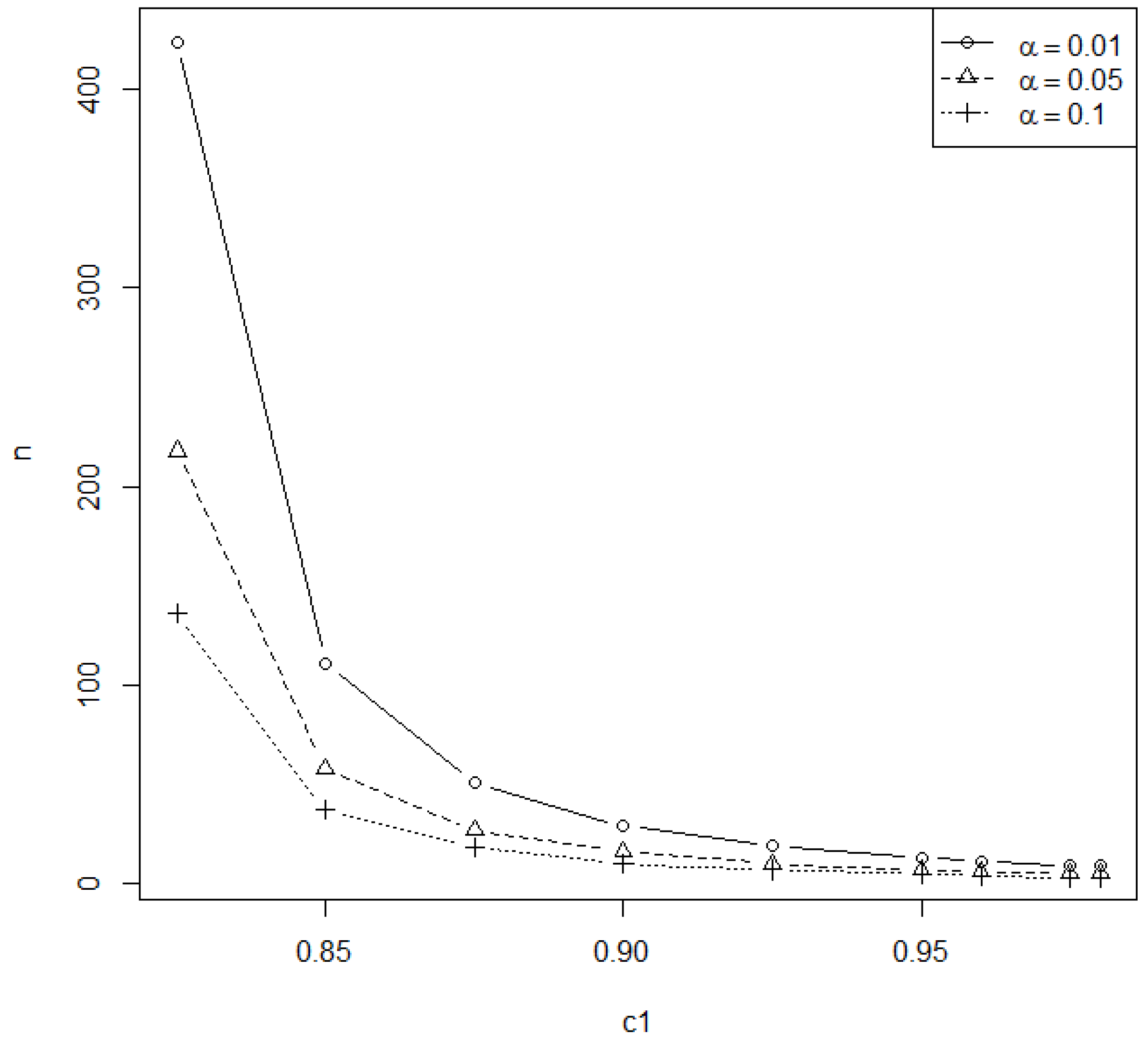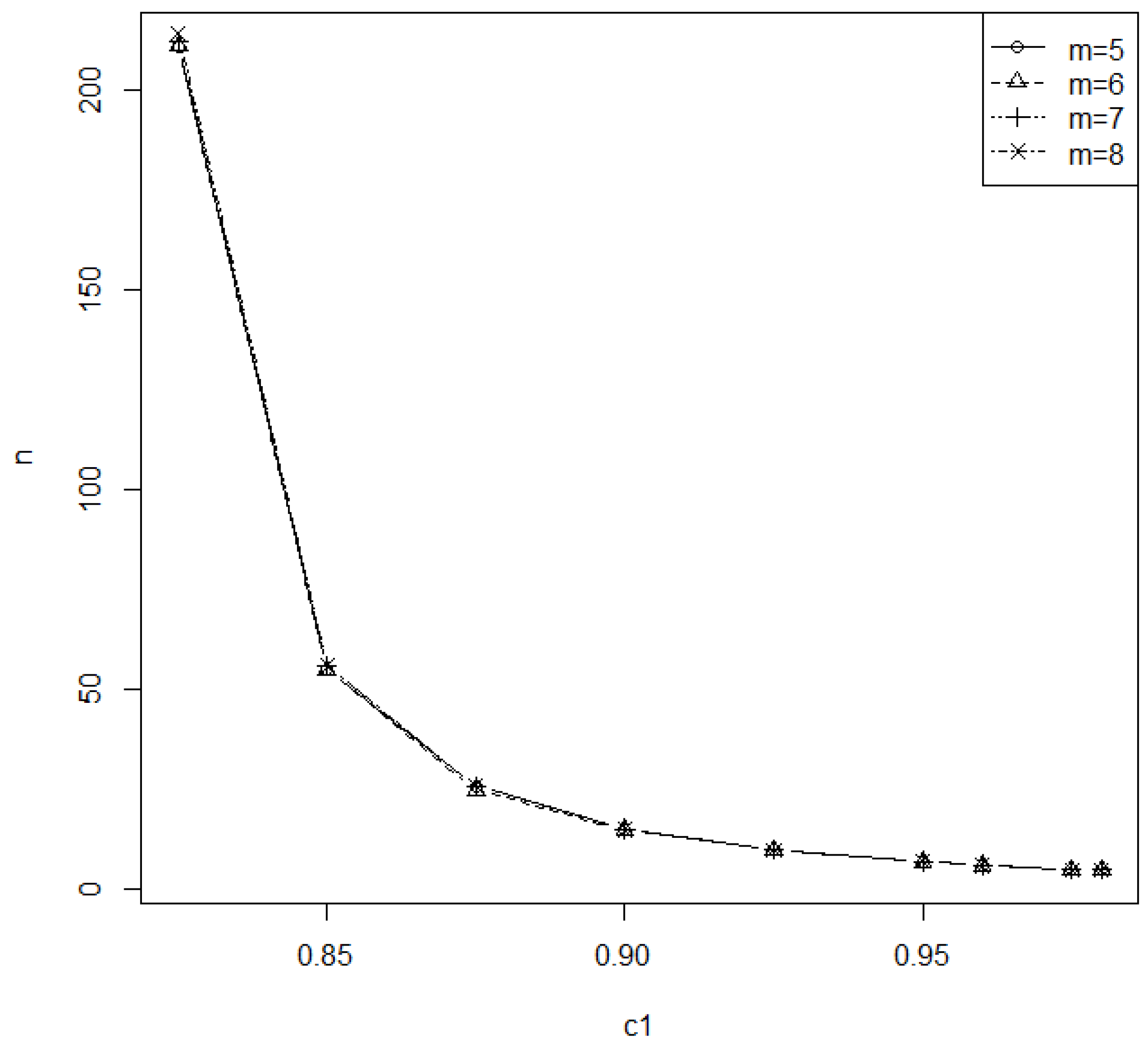The minimum required sample sizes are also displayed in Figure 1, Figure 2, Figure 3 and Figure 4 for some typical cases. Observed in Figure 1, Figure 2, Figure 3 and Figure 4, we find that (1) the minimum sample size n is a decreasing function of c₁ for fixed α, β, m and p; (2) the minimum sample size is a decreasing function of the level of significance for fixed β, m and p; (3) the minimum sample size is a nondecreasing function of m at α = 0.05 for a fixed β = 0.2 and p = 0.05; (4) the minimum sample size is a nonincreasing function of the removal percentage p for fixed α, β and m and (5) the minimum sample size is a decreasing function of power 1-β at α = 0.05 for fixed m = 5 and p = 0.05.

3.2. The Determination of Optimal m and n When the Termination Time Is Fixed

The smaller the number of inspection intervals m, the more convenient for experimenters to collect a progressive type I interval sample. There must be an upper limit m₀ for m specified by the experimenters (The default value of m₀ is 100). In this subsection, the case of the fixed termination time is considered. For this case, the algorithm for searching the optimal (m,n) is presented so that the total experimental cost is minimized for the testing procedure in Wu and Lin [15] under progressive type I interval censoring. Using the cost structure in Huang and Wu [19], the following costs are considered:

• C_a: The cost of installing all test units;
• C_s: The cost for per test unit in the sample;
• C_I: The cost for the use of the inspection equipment;
• C_o: The cost for operating the equipment per unit of experimental time.

Integrating all these costs, we have the total cost of

TC(m,n) = C_a + nC_s + m C_I + T C_o

(11)

where n is determined in Equation (10).

The Algorithm 1 using the numeration method to search the optimal (m,n) is given as follows:

Algorithm 1:

Step 1: Give the preassigned values of c0, c1, α, β, p, T, L and m0 (the default value is 100) and the four costs Ca = aCo, Cs = bCo, CI = cCo and Co by the experimenters.

Step 2: Set m = 1.

Step 3: Compute the sample size n in Equation (10) as n’(m) and then compute the corresponding total cost TC(m, n’(m)), as in Equation (11).

Step 4: If m ≥ m0, then go to Step 5; otherwise, m = m + 1, and go to Step 3.

Step 5: The optimal solution of m* is the minimum m value with the minimum total cost TC(m, n’(m)). Then, the corresponding sample size n* = n’(m*) is obtained.

Step 6: Calculate the critical value of $C_L^0=1-L(k_0+Z_{\alpha }\sqrt{I^{-1}(k_0)})$ by replacing m = m* and n = m*.

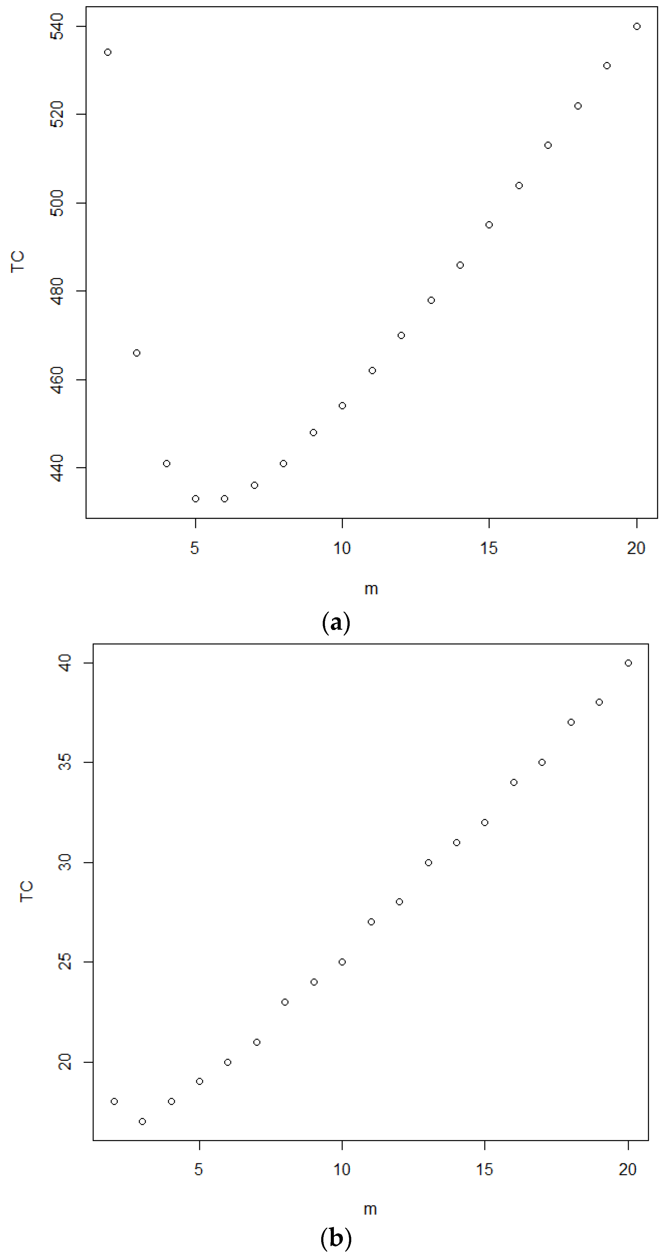
Consider C_o = 1 and a = b = c = 1 and testing for $H_0:C_L\le 0.8$. When β = 0.15, α= 0.01, p = 0.05, $\delta$ = 1.97, c₁ = 0.825, m₀ = 20, L = 0.3 and T = 3.0, the curve of the total cost versus m = 2:m₀ is plotted in Figure 5a. From this figure, it can be seen that the total cost curve is a convex curve, and the minimum number of inspection intervals is m = 5, with a minimum total cost of 424. For another setup of parameters β = 0.25, α = 0.1, p = 0.1, $\delta$ = 1.97, c₁ = 0.90, m₀ = 20, L = 0.3 and T = 3.0, the plot of m = 2:m₀ against its corresponding total cost is made in Figure 5b. This figure also shows that it is a convex curve with some flats, and the minimum number of inspection intervals is m = 3, with a minimum total cost of 17.

Consider the case of β = 0.25, 0.20 and 0.15, α = 0.01, 0.05 and 0.1; L = 0.3; T = 3.0; p = 0.05, 0.075 and 0.1 and testing $H_0:C_L\le 0.8$. The required inspection intervals m* and sample size n* to yield the minimum total cost TC(m*,n*) under m₀ = 20 are tabulated in

Table 4. The optimal (m*,n*), total cost TC and critical value $C_L^0$ for c₁ = 0.825 and 0.850 and p = 0.05, 0.075 and 0.1 under α = 0.1, L = 0.3, T = 3.0 and c₀ = 0.8.

		c1			0.825				0.85
α	β	p	$m^{*}$	$n^{*}$	$TC$	$C_L^0$	$m^{*}$	$n^{*}$	$TC$	$C_L^0$
0.01	0.25	0.050	5	415	424	0.77781	5	107	116	0.75644
		0.075	5	429	438	0.77915	4	112	120	0.75884
		0.100	4	443	451	0.78035	4	114	122	0.76142
	0.20	0.050	5	419	428	0.77792	5	109	118	0.75677
		0.075	5	433	442	0.77925	4	114	122	0.75911
		0.100	4	447	455	0.78046	4	116	124	0.76174
	0.15	0.050	5	424	433	0.77805	5	111	120	0.75725
		0.075	5	438	447	0.77937	4	116	124	0.75963
		0.100	4	452	460	0.78057	4	119	127	0.76215
0.05	0.25	0.050	5	211	220	0.77801	5	55	64	0.75693
		0.075	5	218	227	0.77932	4	58	66	0.75950
		0.100	4	225	233	0.78052	4	59	67	0.76205
	0.20	0.050	5	214	223	0.77818	4	58	66	0.75714
		0.075	5	221	230	0.77949	4	59	67	0.76000
		0.100	4	229	237	0.78068	4	60	68	0.76246
	0.15	0.050	5	218	227	0.77834	4	59	67	0.75775
		0.075	5	225	234	0.77966	4	61	69	0.76049
		0.100	4	232	240	0.78084	4	62	70	0.76304
0.10	0.25	0.050	5	131	140	0.77822	4	35	43	0.75720
		0.075	4	136	144	0.77944	4	36	44	0.75993
		0.100	4	139	147	0.78070	3	38	45	0.76172
	0.20	0.050	5	133	142	0.77842	4	37	45	0.75818
		0.075	5	137	146	0.77970	4	37	45	0.76073
		0.100	4	142	150	0.78088	4	38	46	0.76308
	0.15	0.050	5	136	145	0.77862	4	38	46	0.75865
		0.075	5	140	149	0.77992	3	40	47	0.76054
		0.100	4	145	153	0.78109	3	41	48	0.76330

and

Table 5. The optimal (m*,n*), total cost TC and critical value $C_L^0$ for c₁ = 0.875 and 0.90 and p = 0.05, 0.075 and 0.1 under L = 0.3, T = 3.0 and c₀ = 0.8.

		c1			0.875				0.90
α	β	p	$m^{*}$	$n^{*}$	$TC$	$C_L^0$	$m^{*}$	$n^{*}$	$TC$	$C_L^0$
0.01	0.25	0.050	4	50	58	0.73444	4	28	36	0.71364
		0.075	4	51	59	0.73871	3	30	37	0.71755
		0.100	4	52	60	0.74280	3	31	38	0.72265
	0.20	0.050	4	51	59	0.73553	4	29	37	0.71488
		0.075	4	52	60	0.73958	3	31	38	0.71856
		0.100	4	53	61	0.74350	3	31	38	0.72348
	0.15	0.050	4	52	60	0.73605	3	31	38	0.71361
		0.075	4	53	61	0.74041	4	30	38	0.72144
		0.100	4	54	62	0.74416	3	32	39	0.72505
0.05	0.25	0.050	3	27	34	0.73418	3	16	23	0.71362
		0.075	3	28	35	0.73855	3	16	23	0.71954
		0.100	3	28	35	0.74276	3	16	23	0.72428
	0.20	0.050	3	28	35	0.73521	3	16	23	0.71592
		0.075	4	27	35	0.74082	3	16	23	0.72139
		0.100	3	29	36	0.74408	3	17	24	0.72581
	0.15	0.050	3	29	36	0.73620	3	17	24	0.71592
		0.075	4	28	36	0.74236	3	17	24	0.72312
		0.100	3	30	37	0.74470	3	17	24	0.72725
0.10	0.25	0.050	3	17	24	0.73615	3	10	17	0.71390
		0.075	3	18	25	0.74010	3	10	17	0.72033
		0.100	3	18	25	0.74438	3	10	17	0.72775
	0.20	0.050	3	18	25	0.73769	2	12	18	0.71155
		0.075	3	18	25	0.74136	2	12	18	0.71803
		0.100	3	19	26	0.74538	2	12	18	0.72325
	0.15	0.050	3	19	26	0.73769	2	12	18	0.71502
		0.075	3	19	26	0.74255	2	12	18	0.72081
		0.100	3	19	26	0.74633	3	11	18	0.72991

for c₁ = 0.825 and 0.850 and c₁ = 0.875 and 0.90, respectively. We also tabulated the related critical values in these two tables. Suppose that the experimenters would like to conduct a level 0.05 test for the case of 1-β = 0.8 at c₁ = 0.90, p = 0.05 and m₀ = 20. We can find the minimum number of inspection intervals to be three, with the minimum total cost 23 from Table 5. At the same time, the corresponding required sample size can be 16, with the critical value 0.71592.

We have the following findings from Table 4 and Table 5: (1) the minimum required sample size is a nonincreasing function of the level of significance for fixed β and p; (2) the minimum required sample size is a nonincreasing function of c₁ for fixed α, β and p; (3) the minimum required sample size increases when the probability of type II error β decreases; (4) the minimum inspection intervals decrease when c₁ increases for any combination of α, β and p; (5) the minimum inspection intervals increases when the probability of type II error β decreases; (6) the minimum total cost increases when the removal probability p decreases for fixed α, β and c₁ are fixed; (7) the minimum total cost decreases when c₁ increases for any combination of α, β and p and (8) the minimum total cost increases when the probability of type II error β decreases.

3.3. The Determination of Optimal m, t and n for the Unfixed Total Life Test Time T

In this subsection, the case of the fixed termination time T and unfixed equal interval length t is considered. The algorithm for searching the optimal (m,t,n) is presented so that the total experimental cost is minimized for the testing procedure based on Wu and Lin [15] under progressive type I interval censoring.

The total cost is

TC(m,t,n) = C_a + nC_s + m C_I + mt C_o

(12)

where n is determined in Equation (10).

The Algorithm 2 using the numeration method to search the optimal (m,t,n) is given as follows:

Algorithm 2:

Step 1: Give the preassigned values of c0, c1, α, β, p, T, L and m0 (the default value is 100) and the four costs Ca = aCo, Cs = bCo, CI = cCo and Co by the experimenters.

Step 2: Set m = 1.

Step 3: Find the optimal solution t*, such that TC(m,t,n) is minimized. Compute the sample size n in Equation (10) as n′(m,t*), and then, compute the corresponding total cost TC(m,t*, n’(m,t*)), as in Equation (12).

Step 4: If m ≥ m0, then go to Step 5; otherwise, m = m+1, and go to Step 3.

Step 5: The optimal solution of m* is the minimum m value with the minimum total cost TC(m, n’(m)). Then, the corresponding sample size n* = n’(m*) is obtained.

Step 6: Calculate the critical value of $C_L^0=1-L(k_0+Z_{\alpha }\sqrt{I^{-1}(k_0)})$ by replacing m = m* and n = m*.

Consider the cost structure C_o = 1 and a = b = c = 1 and the testing for $H_0:C_L\le 0.8$. When β = 0.25, α = 0.01, p = 0.05, $\delta$ = 1.97, c₁ = 0.825, m₀ = 20, L = 0.3 and T = 3.0, the curve of total cost versus m = 2:m₀ is plotted in Figure 6a. It can be seen that the total cost curve is a convex curve, and the minimum number of inspection intervals is m = 6, with a minimum total cost of 423.1605. For another set up of parameters: β = 0.15, α = 0.1, p = 0.1 and c₁ = 0.90, the plot of the total cost curve with m = 1:m₀ is made in Figure 6b. It can be seen that the total cost curve is a concave upward curve, and the minimum number of inspection intervals is m = 3, with a minimum total cost of 16.8.

Consider the case of β = 0.25, 0.20 and 0.15; α = 0.01, 0.05 and 0.1; L = 0.3; T = 3.0; p = 0.05, 0.075 and 0.1 and c₀ = 0.8. The minimum suggested number of inspection intervals m*, optimal equal interval length t* and sample size n* to attain the minimum total cost TC(m*,t*,n*) under m₀ = 20 are tabulated in

Table 6. The optimal (m*,t*,n*), total cost TC and critical value $C_L^0$ for c₁ = 0.825 and 0.850 and p = 0.05, 0.075 and 0.1 under L = 0.3, T = 3.0 and c₀ = 0.8.

		c1			0.825					0.85
α	β	p	$m^{*}$	$t^{*}$	$n^{*}$	$TC$	$C_L^0$	$m^{*}$	$t^{*}$	$n^{*}$	$TC$	$C_L^0$
0.01	0.25	0.050	6	0.53	413	423.161	0.77552	5	0.53	107	115.659	0.75198
		0.075	5	0.6	428	437.004	0.77552	4	0.65	111	118.591	0.75177
		0.100	4	0.68	442	449.702	0.77549	4	0.66	114	121.637	0.75177
	0.20	0.050	5	0.55	419	427.759	0.77558	4	0.62	110	117.481	0.75218
		0.075	5	0.58	433	441.877	0.77562	4	0.64	113	120.568	0.75218
		0.100	5	0.65	445	454.226	0.77565	4	0.66	116	123.639	0.75219
	0.15	0.050	5	0.55	424	432.761	0.77573	5	0.54	111	119.696	0.75287
		0.075	5	0.58	438	446.905	0.77576	4	0.6	116	123.406	0.75267
		0.100	4	0.67	452	459.688	0.77576	3	0.8	120	126.399	0.75266
0.05	0.25	0.050	5	0.55	211	219.725	0.77573	4	0.58	56	63.319	0.75248
		0.075	4	0.66	219	226.654	0.77567	3	0.71	59	65.117	0.75251
		0.100	4	0.66	225	232.65	0.77573	3	0.73	60	66.186	0.75249
	0.20	0.050	5	0.55	214	222.744	0.77590	4	0.62	57	64.482	0.75303
		0.075	5	0.58	221	229.912	0.77590	3	0.74	60	66.231	0.75264
		0.100	4	0.68	228	235.713	0.77590	3	0.7	62	68.097	0.75346
	0.15	0.050	5	0.53	218	226.641	0.77605	4	0.58	59	66.324	0.75370
		0.075	4	0.65	226	233.607	0.77605	3	0.72	62	68.155	0.75373
		0.100	4	0.67	232	239.668	0.77610	3	0.75	63	69.244	0.75371
0.10	0.25	0.050	4	0.6	132	139.4	0.77574	3	0.71	36	42.12	0.75316
		0.075	4	0.6	136	143.414	0.77592	3	0.69	37	43.072	0.75315
		0.100	4	0.65	139	146.607	0.77592	3	0.68	38	44.048	0.75375
	0.20	0.050	5	0.52	133	141.595	0.77615	3	0.72	37	43.172	0.75384
		0.075	4	0.63	138	145.508	0.77615	3	0.71	38	44.115	0.75390
		0.100	4	0.63	142	149.522	0.77606	3	0.7	39	45.089	0.75391
	0.15	0.050	4	0.62	137	144.478	0.77640	3	0.66	39	44.995	0.75408
		0.075	4	0.62	141	148.496	0.77639	3	0.75	39	45.257	0.75521
		0.100	4	0.63	145	152.527	0.77631	3	0.73	40	46.195	0.75576

and

Table 7. The optimal (m*,t*,n*), total cost TC and critical value $C_L^0$ for c₁ = 0.875 and 0.90 and p = 0.05, 0.075 and 0.1 under L = 0.3, T = 3.0 and c₀ = 0.8.

		c1			0.825					0.85
α	β	p	$m^{*}$	$t^{*}$	$n^{*}$	$TC$	$C_L^0$	$m^{*}$	$t^{*}$	$n^{*}$	$TC$	$C_L^0$
0.01	0.25	0.050	4	0.61	49	56.451	0.72832	3	0.69	29	35.065	0.70665
		0.075	3	0.7	52	58.109	0.72837	3	0.66	30	35.99	0.70658
		0.100	3	0.72	53	59.149	0.72843	3	0.73	30	36.19	0.70652
	0.20	0.050	4	0.63	50	57.518	0.72910	3	0.66	30	35.994	0.70618
		0.075	3	0.72	53	59.145	0.72922	3	0.74	30	36.225	0.70607
		0.100	3	0.73	54	60.191	0.72917	3	0.7	31	37.108	0.70764
	0.15	0.050	3	0.73	53	59.196	0.73004	3	0.66	31	36.969	0.70618
		0.075	3	0.75	54	60.253	0.73003	3	0.72	31	37.16	0.70745
		0.100	4	0.68	54	61.721	0.73061	3	0.69	32	38.083	0.70890
0.05	0.25	0.050	3	0.64	27	32.928	0.73102	3	0.71	15	21.138	0.70983
		0.075	3	0.7	27	33.102	0.73098	3	0.62	16	21.875	0.71470
		0.100	3	0.67	28	34.006	0.72980	3	0.67	16	22.002	0.71478
	0.20	0.050	3	0.74	27	33.217	0.73198	3	0.64	16	21.918	0.70875
		0.075	3	0.69	28	34.055	0.73209	3	0.69	16	22.07	0.71380
		0.100	3	0.66	29	34.984	0.73086	3	0.63	17	22.879	0.71151
	0.15	0.050	3	0.73	28	34.192	0.73313	3	0.75	16	22.255	0.71274
		0.075	3	0.69	29	35.06	0.73323	3	0.65	17	22.942	0.71311
		0.100	3	0.67	30	35.996	0.73218	3	0.7	17	23.089	0.71525
0.10	0.25	0.050	3	0.64	17	22.924	0.73297	3	0.6	10	15.815	0.70895
		0.075	3	0.7	17	23.092	0.73472	3	0.64	10	15.925	0.71318
		0.100	3	0.63	18	23.896	0.73289	3	0.69	10	16.068	0.71678
	0.20	0.050	3	0.61	18	23.843	0.73237	3	0.68	10	16.032	0.71495
		0.075	3	0.66	18	23.966	0.73426	3	0.76	10	16.27	0.71827
		0.100	3	0.71	18	24.138	0.73573	3	0.61	11	16.826	0.71497
	0.15	0.050	3	0.71	18	24.122	0.73553	3	0.61	11	16.815	0.71349
		0.075	3	0.64	19	24.92	0.73561	3	0.64	11	16.919	0.71687
		0.100	3	0.69	19	25.063	0.73709	3	0.68	11	17.05	0.72543

for c₁ = 0.825 and 0.850 and c₁ = 0.875 and 0.90, respectively. We also list the critical values $C_L^0$ in these two tables. If the experimenters would like to conduct a level 0.05 test under the conditions of β = 0.8, c₁ = 0.825, p = 0.05 and m₀ = 20, the optimal values of (m*,t*,n*) can be found as (5,0.55,214) from Table 6. From this table, you can also find the minimum total cost as TC = 222.744 and the corresponding critical value as 0.7759.

A software program to find the optimal setup for the sampling design proposed in Section 3.1, Section 3.2 and Section 3.3 for any combination of parameters was built by the authors for practical use.

From Table 6 and Table 7, we have the following findings: (1) the minimum required sample size is a decreasing function of the level of significance for fixed β and p; (2) the minimum required sample size is a decreasing function of c₁ for fixed α, β and p; (3) the minimum required sample size increases when the probability of a type II error β decreases; (4) the minimum number of inspection intervals decreases when c₁ increases for any combinations of α, β and p; (5) the minimum number of inspection intervals increases when the probability of a type II error β decreases; (6) the minimum total cost decreases when c₁ increases for fixed α, β and p; (7) the minimum total cost increases when the probability of a type II error β decreases and (8) the minimum total cost is a nonincreasing function of the removal probability p for fixed α, β and c₁.

3.4. Example

For the aims of the illustration, the data in Caroni [20] is used to illustrate our proposed sampling design. The data of the failure times of n = 25 ball bearing are given as follows (number of cycles in 1000 times): 0.1788, 0.2892, 0.3300, 0.4152, 0.4212, 0.4560, 0.4848, 0.5184, 0.5196, 0.5412, 0.5556, 0.6780, 0.6780, 0.6780, 0.6864, 0.6864, 0.6888, 0.8412, 0.9312, 0.9864, 1.0512, 1.0584, 1.2792, 1.2804, 1.7340.

The Gini test (see Gail and Gastwirth [21]) is a scale-free goodness-of-fit test for distribution that can be transformed into an exponential distribution. The testing procedures in Jäntschi [22] and Jäntschi [23] are more general procedures as alternatives to the Gini test. We use the Gini test with the maximum p-value to determine the parameter δ for this example. We conduct the Gini test as follows: In the first step, the null hypothesis is set up as $H_{:0}:U_i~F_U(u)=1-\exp \left\{-{(\frac{u}{\lambda })}^{\delta }\right\},u>0,\delta >0,\lambda >0$. Secondly, we sort the data in order as U₍₁₎ = 0.1788, U₍₂₎ = 0.2892,… and U₍₂₅₎ = 1.7340. We calculate the Gini test statistic $G_n=\frac{{\displaystyle \sum _{i=1}^{n-1}i(n-i)(Y_{(i+1)}-Y_{(i)})}}{24{\displaystyle \sum _{i=1}^n(n-i+1)(Y_{(i)}-Y_{(i-1)})}}$, where $Y_{(i)}=U_{(i)}^{\delta }$. The limiting distribution of $Z=\sqrt{12(n-1)}(G_n-0.5)$ is a standard normal distribution when the sample size is large enough. Let z be the realization of Z, and then, the p-value is obtained as $2P(Z>|z|)$. The higher the p-value, the better fit of the data to the Weibull distribution. From Wu and Lin [15], the value of δ is determined as δ = 1.97, since it has the largest p-value = 0.9882 for the Gini test. With a high p-value, we conclude that the data fits the Weibull distribution very well. We then used this example to illustrate Section 3.1, Section 3.2 and Section 3.3.

For Section 3.1, we considered the case of L = 0.05, T = 0.5, m = 5 and p = 0.05 for testing $H_0:C_L\le 0.8$ with a significance level α = 0.05 and the power level 1-β = 0.75 at c₁ = 0.975. After running our software, the minimum sample size was determined to be n = 20, and the critical value was obtained as $C_L^0$ = 0.7002605.

Then, the hypothesis test was conducted as follows:

Step 1: We took a random sample of size n = 20 from the dataset. The progressive type I interval censored sample (X₁,X₂,…,X₅) = (0,1,1,1,2) was collected at the time points (t₁,t₂,…,t₅) = (0.1,0.2,0.3,0.4,0.5) under the progressive censoring scheme of (R₁,R₂,…,R₅) = (1,2,0,2,10).

Step 2: Based on the progressive type I interval censored sample given in step 1, the MLE of k was found to be $\widehat{k}$ = 1.382812 by solving Equation (6).

Step 3: The value of test statistic ${\widehat{C}}_L=1-\widehat{k}L$ = 1 − 1.382812 × 0.05 = 0.9308594 was computed.

Step 4: Due to the result of ${\widehat{C}}_L$ = 0.9308594 > $C_L^0$ = 0.7002605, we concluded it supported the alternative hypothesis $H_a:C_L>0.8$ and claimed that the lifetime performance index exceeded the desired level.

From Section 3.2, the same consideration of parameters and cost setup as the previous paragraph was considered. After running our software, the minimum number of inspection intervals and the related sample size were determined to be m* = 1 and n*= 19, with the critical value as $C_L^0$ = 0.7228799 and a minimum total cost of 21.5 units.

The, a hypothesis test about $C_L$ was conducted as follows:

Step 1: A random sample of size n = 19 was taken from the dataset. The progressive type I interval censored sample (X₁) = (5) was collected at the time point (t₁) = (0.5) under the progressive censoring scheme of (R₁) = (14).

Step 2: Using the progressive type I interval censored sample collected in step 1, the MLE of k was found to be $\widehat{k}$ = 1.196398 by solving Equation (6).

Step 3: Computing the test statistic, ${\widehat{C}}_L=1-\widehat{k}L$ = 1 − 0.196398 × 0.05 = 0.9401801.

Step 4: We observed that ${\widehat{C}}_L$ = 0.9401801 > $C_L^0$ = 0.7228799. Thus, it supported the alternative hypothesis $H_a:C_L>0.8$ and claimed that the lifetime performance index exceeded the desired level.

For Section 3.3, the case of unfixed m and t was considered. Based on the same setup with the previous two cases, the optimal sampling design with (m*,n*,t*) = (2,12,0.42) was found from the output of our software. The critical value $C_L^0$ = 0.7063278 and the minimum total cost of TC = 15.834 units could also be found from the output.

The testing procedure of $C_L$ was conducted as follows:

Step 1: A random sample of size n = 12 was taken from the dataset. The progressive type I interval censored sample was (X₁,X₂) = (3,6) at the time points (t₁,t₂) = (042,0.84) under the progressive censoring schemes of (R₁,R₂) = (0,3).

Step 2: Based on the progressive type I interval censored sample given in step 1, the MLE of k was found to be $\widehat{k}$ = 1.875922 by solving Equation (6).

Step 3: The test statistic was ${\widehat{C}}_L=1-\widehat{k}L$ = 1 − 1.875922 × 0.05 = 0.9062039.

Step 4: we observed that ${\widehat{C}}_L$ = 0.9062039 > $C_L^0$ = 0.7063278. Based on this observation, the same claim was made with the previous two cases.

4. Conclusions

This model of Weibull distribution is widely used for reliability engineering and failure analyses. The lifetime performance index can be used to assess the capability performance of a manufacturing process, especially for Weibull products. Based on the progressive type I interval censored sample, we investigated the required minimum sample size under a given power for the level α test for testing the capability of the manufacturing process based on the lifetime performance index. We also provided the required minimum sample size and number of inspection intervals when the termination time of the experiment was fixed to reach given power and the minimum total cost for the level α test. When the termination time of the experiment was not fixed, the required minimum sample size, number of inspection intervals and the inspection interval time length were determined in this paper to reach the given power with the minimum total cost for the level α test under progressive type I interval censoring.