Article

Hidden Dynamical Symmetry and Quantum Thermodynamics from the First Principles: Quantized Small Environment

by
Ashot S. Gevorkyan
1,2,*,
Alexander V. Bogdanov
3 and
Vladimir V. Mareev
3
1
Institute for Informatics and Automation Problems NAS of RA, 1, P. Sevak Str., Yerevan 0014, Armenia
2
Institute of Chemical Physics NAS of RA, 5/2, P. Sevak Str., Yerevan 0014, Armenia
3
Faculty of Applied Mathematics and Control Processes, Saint-Petersburg State University, 198504 Saint-Petersburg, Russia
*
Author to whom correspondence should be addressed.
Symmetry 2021, 13(8), 1546; https://doi.org/10.3390/sym13081546
Submission received: 22 June 2021 / Revised: 21 July 2021 / Accepted: 12 August 2021 / Published: 23 August 2021
(This article belongs to the Special Issue Symmetry in Particle Physics II)

Abstract

:
Evolution of a self-consistent joint system (JS), i.e., a quantum system (QS) + thermal bath (TB), is considered within the framework of the Langevin–Schrödinger (L-Sch) type equation. As a tested QS, we considered two linearly coupled quantum oscillators that interact with TB. The influence of TB on QS is described by the white noise type autocorrelation function. Using the reference differential equation, the original L-Sch equation is reduced to an autonomous form on a random space–time continuum, which reflects the fact of the existence of a hidden symmetry of JS. It is proven that, as a result of JS relaxation, a two-dimensional quantized small environment is formed, which is an integral part of QS. The possibility of constructing quantum thermodynamics from the first principles of non-Hermitian quantum mechanics without using any additional axioms has been proven. A numerical algorithm has been developed for modeling various properties and parameters of the QS and its environment.

1. Introduction

When we try to approach the study of a quantum system (QS) strictly and consistently, it becomes obvious that its isolation from the environment is an almost non-realizable task. Note that even if we assume that it is possible to exclude the interaction of QS with the environment, taking into account the influence of quantum fluctuations of vacuum makes the QS an open system in any case [1,2,3,4,5,6]. In other words, a full description of QS also requires the inclusion of its environment, which is essentially the whole universe. Thus, the fact that any QS is in a certain sense an open system means that in reality no quantum state can be a pure state.
In recent years, issues related to taking into account the influence of the environment on the properties of a quantum system have become the subject of increased interest in connection with the importance of solving a number of fundamental and applied problems of science and technology. Recall that the solution of such problems can stimulate the further development of quantum foundations [7,8], discover new possibilities of quantum measurements [9], allow controlling of the processes of dissipation and decoherence [10,11,12,13], clarify the question of how the classical properties forms from the quantum world [14], to better understand the nature of quantum correlations and quantum discord [15], the peculiarities of the entanglement at the Bose condensation [16,17], etc.
As a rule, when we speak about the environment, we usually mean a large system (thermostat or thermal bath (TB)), which is characterized by a finite temperature and distributions of various physical parameters in a state of thermodynamical equilibrium. Recall that the theory of open quantum systems [18,19], which is the basis of almost all modern studies in the field of quantum mechanics and its applications, takes into account the influence of the thermostat on QS, while the effect of QS on the thermostat is not taken into account. This assumption underlying the theory of open QS is justified in many cases. Nevertheless, there are also many cases when the fact of the openness of quantum systems is not simply impossible to neglect, but, on the contrary, must be taken into account with all mathematical rigor. Note that this is especially relevant in the field of quantum information processes, the advantage of which is obvious in comparison with classical information processing [20]. Mathematically, a more rigorous and consistent formulation of open QS is very important for studying the relaxation of not only QS, but also the thermostat itself in order to avoid the loss of information inherent in open systems. In other words, the solution to this problem is to develop a representation that would allow us to consider an open system as a closed one.
Recently, when studying the properties of quantum thermodynamics in the framework of model calculations, it was shown that thermal behavior manifests itself even with sufficiently small entangled quantum systems [7,8]. In particular, calculations show that micro-canonical and thermal behavior have been observed, including the rapid approach to micro-canonical equilibrium entropy that is typical to canonical systems. The results of these numerical simulations are explained theoretically [21], wherein the key role of quantum entanglement between the system and its environment in attainment of thermodynamic equilibrium in the system has been shown. Moreover, it has been proven that the basic postulate of statistical mechanics, namely the postulate of a priori equal probability of statistical states, should be discarded as unnecessary and misleading. In [22], a model system of coupled quantum oscillators was calculated by way of numerical simulation, which interacts with a quantum environment.
The goal of this article is to develop a representation that will allow us to self-consistently study the evolution of JS as a closed, inextricable system depending on time. The physical idea is that we assume that in the process of evolution JS self-organizes and comes to the statistical equilibrium. Mathematically, the problem is formulated within the framework of a complex probabilistic process that satisfies a stochastic differential equation of the Langevin–Schrödinger (L-Sch) type. Using the L-Sch equation as the first principle, we in a closed form, that is, in the form of double integrals and solutions of partial differential equations, construct all the parameters and the corresponding distributions of QS and environmental fields.
The manuscript is organized as follows:
In Section 2, the problem of coupled quantum oscillators is formulated taking into account the presence of a random environment. The existence of a hidden symmetry of the internal motion of the JS is proved, which allows the original equation describing the JS to lead to an autonomous form. The explicit form of the wave function of the joint system (JS) “two coupled quantum oscillators + TB ” is obtained by solving the L-Sch equation in the form of an orthonormal probability processes.
In Section 3, stochastic differential equations (SDE) are obtained that describe the free evolution of the environment or TB. Using these SDEs, second-order partial differential equations (PDEs) were obtained that describe distributions of environmental fields for different scenarios depending on time. To solve these PDFs, the Neumann initial-boundary conditions are formulated.
In Section 4, on the basis of an equation describing the distribution of environmental fields is the obtained difference equation. The evolution of the distribution of environmental fields is simulated for various initial boundary conditions.
In Section 5, a method of stochastic density matrix was developed. It contains the basic definitions with the help of which different statistical distributions and the average values of corresponding parameters of the QS and its small environment are constructed. Conditions are formulated under which the developed quantum representation can be non-Hermitian.
In Section 6, we prove the possibility of the formation of a quantized small environment as a result of the influence of QS on the TB. A number of distributions of the quantized fields of the small environment are calculated and visualized. This section also presents visualizations of calculating the probability density of the first few QS states.
Section 7 is devoted to the analytical construction of nonstationary quantum entropy. In particular, the von Neumann entropy for the “ground state” is analyzed in detail and its generalization is given.
In Section 8, the energy levels and their populations are constructed in the form of two-dimensional integral representations.
Section 9 considers the problem of entanglement of two 1D quantum oscillators as a result of their relaxation in a thermostat. The formation of Bell states is considered in detail. An equation that describes the evolution of the TB under the influence of QS and the formation of the so-called small environment is derived.
In Section 10, the amplitudes of the probabilities of transitions between various asymptotic states of the ( i n ) and ( o u t ) channels are constructed.
In Section 11, the obtained results are discussed in detail and further methods of development of the representation.
If we schematically represent the structure of the study (see Figure 1), then in Section 2, Section 3 and Section 4 we reduce the problem of coupled linear oscillators with a random environment to the problem of two separate one-dimensional oscillators with random environments and we find exact solutions for them. Section 5 contains the basic definitions with the help of which various statistical distributions and average values of the corresponding parameters of the QS and its small environment are constructed. In Section 6, Section 7, Section 8, Section 9 and Section 10 various statistical parameters of the QS and its environment are constructed using the results obtained in Section 2, Section 3 and Section 4 and the definitions of Section 5.

2. Formulation of the Problem

2.1. Hidden Dynamical Symmetry and General Solution of the Wave Function of a JS

Let us consider the JS in the framework of the stochastic differential equation (SDE) of the Langevin–Schrödinger type:
i t Ψ s t c = H ^ x , t ; { f } Ψ s t c , t / t ,
where the wave function Ψ s t c x , t ; { f } represents a complex probability process. As for the operator H ^ ( x , t ; { f } ) describing the Hamiltonian of the JS, in units of = m = 1 it has the following form:
H ^ x , t ; { f } = 1 2 l = 1 2 2 x l 2 + ω ˘ 2 t ; { f } x l 2 + ω t ; { f } x 1 x 2 , x = ( x 1 , x 2 ) R 2 ,
where ω ˘ t ; { f } and ω ( t ; { f } ) are arbitrary functions of time, consisting of both regular and random terms, and { f } denotes some complex stochastic process that will be clearly defined below (see Equation (16)).
Theorem 1.
If the equation of motion of the JS (1) is described by the Hamiltonian (2), then;
a. The motions of the coupled linear oscillators system conditionally can be separated on the motions of two separate 1D oscillators with random environment;
b. The equation of the 1D oscillator immersed in the TB is reduced to an autonomous form with the help of a small dimension reference differential equation, which is solved exactly, in the form of the orthogonal stochastic process.
Proof. 
For analytical investigation of the problem, it is necessary to bring the JS Hamiltonian (2) to a diagonal form.
By performing the following coordinate transformations:
q 1 = x 1 x 2 2 , q 2 = x 1 + x 2 2 , q = ( q 1 , q 2 ) R 2 ,
in Equation (2) we obtain:
H ^ q 1 , q 2 , t ; { f } = 1 2 l = 1 2 2 q l 2 + Ω l 2 t ; { f } q l 2 ,
where Ω l t ; { f } denotes the effective random frequency:
Ω l 2 t ; { f } = ω ˘ 2 t ; { f } ( 1 ) l ω t ; { f } 0 .
As follows from (5), it is necessary to impose a constraint on the function ω t ; { f } to satisfy the inequality | ω t ; { f } | R e [ ω ˘ 2 t ; { f } ] .
The general solution of Equations (1) and (2) is naturally represented in a factorized form:
Ψ s t c ( q , t , { ξ } ) = l = 1 2 Y s t c ( l ) ( q l , t , { ξ l } ) ,
where { ξ } = ( ξ 1 , ξ 2 ) denotes some complex stochastic process, which will be defined below, and Y s t c ( l ) ( q l , t , { ξ l } ) is the time-dependent solution—the wave function of the 1 D quantum harmonic oscillator for an arbitrary frequency Ω l t ; { f } .
The explicit form of this wave function is well known (see for example [23]):
Y s t c ( l ) ( q l , t , { ξ l } ) = 1 σ l exp i 2 σ ˙ l σ l q l 2 χ l , σ ˙ l ( t ) = d σ l ( t ) d t ,
where χ l is the solution of the 1D autonomous Schrödinger equation for the harmonic oscillator, but already on a random space–time continuum { y l , τ l } :
i χ l τ l = 1 2 2 y l 2 + ( Ω l y l ) 2 χ l .
Note that the following notations are made in the Equation (8):
y l = q l σ l , ξ l ( t ) = σ l ( t ) e i γ l ( t ) , τ l = γ l ( t ) Ω l , γ l ( t ) = Ω l t d t σ l 2 ( t ) ,
where the function ξ l ( t ) is a solution to the classical oscillatory equation:
ξ ¨ l + Ω l 2 t ; { f } ξ l = 0 , ξ ˙ l = d ξ l / d t .
Obviously, the Equation (10) (reference equation) and transformations (9), allowing reduction of the Langevin–Schrödinger equation with the Hamiltonian (4) to an autonomous form (8) reflect the fact of the existence of some hidden dynamical symmetry of the internal motion of JS.
Now, taking into account the expressions (6)–(8), we can construct the wave function of the JS:
Ψ s t c ( n | q , t ; { ξ } ) = l = 1 2 Y s t c ( l ) ( n l | q l , t ; { ξ l } ) ,
where
Y s t c ( l ) = g l 2 n l n l ! σ l 1 / 2 exp 1 2 i σ l ˙ σ l Ω l σ l 2 q l 2 i n l + 1 2 Ω l t d t σ l 2 H n l Ω l q l σ l ,
In addition, n = (n1, n2) denotes the vibrational quantum numbers of 1D oscillators, Ω l = lim t Ω l ( t ; { f } ) = const—the frequency of the 1D oscillator in an asymptomatic state when the environment is turned off, g l = ( Ω l / π ) 1 / 2 and Hn(x)—the Hermitian polynomial.
The full wave functions Ψ s t c ( n | q , t ; { ξ } ) describing the JS in the Hilbert space form a full orthonormal basis:
Ψ s t c ( n | q , t ; { ξ } ) Ψ s t c ( m | q , t ; { ξ } ) d q = l = 1 2 δ n l m l ,
where δ n l m l denotes the Kronecker symbol.
Recall that the full wave functions are in fact orthogonal random processes. In addition, Ψ s t c ( n | q , t ; { ξ } ) L 2 ( Ξ ) , where Ξ R 2 R { ξ } is the extended space and { ξ } = ( ξ 1 ( t ) , ξ 2 ( t ) ) R { ξ } denotes some functional space, the measure of which can be exactly determined (see [4,24]). The theorem is proved. □

2.2. Determination of the Asymptotic Conditions of the Problem

For further analytical constructions of the problem, it is necessary to refine the a asymptotic properties of the wave function of the unified system.
For definiteness, we will represent the effective frequency as a sum:
Ω l 2 t ; { f } = Ω 0 l 2 ( t ) + f l ( t ) , { f } = { f 1 ( t ) , f 2 ( t ) } .
Note that Ω 0 l ( t ) is a real regular function while f l ( t ) = f l ( r ) ( t ) + i f l ( i ) ( t ) is a random complex function, where f l ( r ) and f l ( i ) ( t ) denote its real and imaginary parts, respectively. In other words, the function f l ( t ) describes the behavior of the TB. Recall that the set of harmonic oscillators [25,26,27,28,29], which is equivalent to the quantized fields [30,31], is often used as a model of the environment or a measuring apparatus that is linearly related to the measured quantum system [32].
Obviously, when the random environment is turn off, the expression (4) is a regular operator or Hamiltonian of a system of coupled 1 D quantum oscillators:
H ^ 0 q 1 , q 2 , t = H ^ q 1 , q 2 , t ; { f } | { f } 0 = 1 2 l = 1 2 2 q l 2 + Ω 0 l 2 ( t ) q l 2 ,
and, accordingly, we are dealing with the usual problem of a parametric quantum oscillator.
We suppose that the functions Ω 0 l ( t ) and f l ( t ) satisfy the following asymptotic conditions:
lim t Ω 0 l ( t ) = Ω l = c o n s t > 0 , lim t f l ( t ) = 0 .
In addition, we assume that f l ( υ ) ( t ) , υ = ( r , i ) , is an independent Gaussian process with zero mean value and a delta-like correlation function [33]:
E f l ( υ ) ( t ) = 0 , E f l ( υ ) ( t ) f l ( υ ) ( t ) = 2 ϵ l ( υ ) δ ( t t ) ,
where E denotes the mathematical expectation of a random variable.
Note that ϵ l ( υ ) denotes the fluctuations power of the environment fields or TB fluctuations. Recall that for ordinary condensed media it is natural to assume that the constant ϵ l ( r ) = ϵ ¯ l = k T l characterizes elastic collisions in TB, where k and T l are the Boltzmann constant and the temperature of TB, respectively. As regards the constant ϵ l ( i ) = μ ϵ l ( r ) = μ ϵ ¯ l , then it characterizes dissipation processes or inelastic collisions in TB. It is assumed that μ is a positive constant. In the case when ϵ 1 ϵ 2 and ϵ l = ϵ l ( r ) , ϵ l ( i ) , in thermodynamic equilibrium the TB can be characterized by two temperatures.
Obviously, the solution to the Equations (1) and (2) in the limit t or in the ( i n ) asymptotic channel can be represented in the factorized form:
Φ i n ( n | q , t ) = l = 1 2 e i ( n l + 1 / 2 ) Ω l t ϕ n l ( q l ) , n l = 0 , 1 , ,
where n ( n 1 , n 2 ) and q ( q 1 , q 2 ) , in addition:
ϕ n l ( q l ) = g l 2 n l n l ! 1 / 2 exp 1 2 Ω l q l 2 H n l Ω l q l , g l = Ω l π 1 / 2 .
Recall that ϕ n l ( q l ) is the wave function of a 1D stationary quantum harmonic oscillator.

3. Fields Equations and Formulation of Their Initial-Boundary Conditions

3.1. Distribution of Fields in the Limit of Statistical Equilibrium

As we saw above, the reference Equation (10), which describes the stochastic fields of the environment, plays a key role in bringing the equation of motion to an autonomous form, but it is not clearly formulated in this form.
Theorem 2.
If the random forces in the system of stochastic Equation (22) satisfy white noise correlation relations (16), then;
a. The environmental fields will be described by two two-dimensional Fokker–Planck equations (in the case of independent sources), and, accordingly,
b. All four fields will be described by one four-dimensional Fokker–Planck equation, when f 1 ( r ) = f 2 ( r ) and f 1 ( i ) = f 2 ( i ) , i.e., the source of random forces is the same for both oscillators.
Proof. 
The solution of the classical Equation (10) can be represented in the form:
ξ l ( t ) = { ξ 0 l ( t ) , t t 0 , ξ 0 l ( t 0 ) exp Θ l ( t ) , t > t 0 ,
where ξ 0 l ( t ) is the solution of the classical oscillator Equation (10) for the regular frequency Ω 0 l ( t ) and Θ l ( t ) = t 0 t ϕ l ( t ) d t . Furthermore, for certainty, we will assume that the turn-on time of the random environment or TB is equal to t 0 = 0 .
Substituting (19) into (10), we obtain the following nonlinear complex SDE:
ϕ l ˙ + ϕ l 2 + Ω 0 l 2 ( t ) + f l ( t ) = 0 ,
where ϕ l ˙ = d ϕ l / d t and ϕ l ( t 0 ) = i Ω l .
Let us represent the complex function ϕ l ( t ) as a sum:
ϕ l ( t ) = u 1 ( l ) ( t ) + i u 2 ( l ) ( t ) ,
where the fields u 1 ( l ) ( t ) , u 2 ( l ) ( t ) R 2 ( , + ) × ( 0 , ) .
Using (21) and (20), we can write the following system of nonlinear SDEs:
{ u ˙ 1 ( l ) = u 2 ( l ) 2 u 1 ( l ) 2 Ω 0 l 2 ( t ) f l ( r ) ( t ) , u ˙ 2 ( l ) = 2 u 1 ( l ) u 2 ( l ) f l ( i ) ( t ) ,
where the environmental fields u ( t ) = [ u 1 ( 1 ) ( t ) , u 2 ( 1 ) ( t ) ] ; [ u 1 ( 2 ) ( t ) , u 2 ( 2 ) ( t ) ] satisfy the following asymptotic conditions:
u ˙ 1 ( l ) ( t 0 ) = R e [ ξ ˙ l ( t 0 ) / ξ l ( t 0 ) ] = 0 , u ˙ 2 ( l ) ( t 0 ) = I m [ ξ ˙ l ( t 0 ) / ξ l ( t 0 ) ] = Ω l .
Note that depending on the character of random forces f 1 ( t ) and f 2 ( t ) , the probabilistic processes (fields) ϕ 1 ( t ) and ϕ 2 ( t ) can be implemented by two different scenarios. Using stochastic differential Equation (22), we can find the probability distribution of the environment fields:
a. When the fields are generated by one source of random forces { f } and, accordingly;
b. When fields are generated by two independent sources of random forces f 1 ( t ) and f 2 ( t ) .
Let us consider the first scenario. In this case, it is obvious that the distribution of TB fields should be represented as follows (see in detail [34,35]):
P ( u , t | u 0 , t 0 ) = l = 1 2 j = 1 2 δ u j ( l ) ( t ) u 0 j ( l ) ,
where u 0 j ( l ) = u j ( l ) ( t 0 ) is the field component in the ( i n ) state.
To simplify the notation, the superscripts of the random fields are omitted in the equations below.
Using the stochastic differential equations in (22) for the probability distribution of the environmental fields, we can find the following Fokker–Planck equation:
t P = l = 1 2 L ^ l Ω 0 l ( t ) , ϵ l | u 1 , u 2 , t P ,
where the evolution operator L ^ l Ω 0 l ( t ) , ϵ l | u 1 , u 2 , t has the form:
L ^ l = ϵ ¯ l 2 u 1 2 + μ 2 u 2 2 + u 1 u 1 2 u 2 2 + Ω 0 l 2 ( t ) + 2 u 1 u 2 u 2 .
Recall that in the Equation (24) u 1 and u 2 are equilibrium fields of the environment or just coordinates that are defined in the following limits u 1 ( , + ) and u 2 ( 0 , + ) .
To solve the Equation (24), it will be naturally to formulate the Dirichlet problem with the following initial-boundary conditions:
P ( u , u 0 , t 0 ) = l = 1 2 j = 1 2 δ ( u j ( l ) ( t ) u 0 j ( l ) ) , P ( u , u 0 , t ) | | | u | | 0 ,
where | | u | | = l = 1 2 { ( u 1 ( l ) ) 2 + ( u 2 ( l ) ) 2 } , in addition, the function P ( u , u 0 , t ) makes sense of the probability distribution of the environmental fields and, accordingly, can be normalized to unity.
In the case of the second scenario, it is natural to assume that the fields distributions will be factorized:
P ( u , t | u 0 , t 0 ) = l = 1 2 P l = l = 1 2 j = 1 2 δ u j ( l ) ( t ) u 0 j ( l ) ,
where the following Fokker–Planck equation for the field distribution can be obtained in a standard way:
t P l = L ^ l Ω 0 l ( t ) , ϵ l | u 1 , u 2 , t P l .
The theorem is proved. □
Thus, at the limit of statistical equilibrium, four additional dimensions arise that describe the fields of the environment and, accordingly, then the original problem becomes six-dimensional R 2 R c 4 , where R c 4 is a compact space and u 1 ( 1 ) , u 2 ( 1 ) , u 1 ( 2 ) , u 2 ( 2 ) R c 4 .

3.2. Neumann Initial-Boundary Conditions

Now let us dwell in detail on the question of setting the initial-boundary value problem for solving Equation (27).
Let, at the initial moment of time t 0 = 0 , the probability distribution of free fields of the environment be described by the Dirac delta functions:
P l ( u 1 , u 2 , t 0 ) = j = 1 2 δ ( u j u 0 j ) .
As for the boundary conditions, then, based on the fact that the QS in TB can be subject to both elastic and inelastic collisions, it is useful to use Neumann conditions of the form:
u 2 P l ( u 1 , u 2 , t ) | u 2 = 0 = 1 P l ( u 1 , t ) 0 , u 1 P l ( u 1 , u 2 , t ) | u 1 = 0 = 2 P l ( u 2 , t ) 0 .
As we will see below, the conditions (29) lead to the fulfilment of two different equations on the axes u 1 and u 2 , respectively. In particular, taking into account that the Equation (27) is invariant under the transformation u 2 u 2 , near the axis u 1 ( , + ) the solution to the equation can be represented as:
P l ( u 1 , u 2 , t ) | u 2 0 a 0 + a 1 u 2 + a 2 u 2 2 + e u 2 2 / 2 1 P l ( u 1 , t ) ,
where a 0 , a 1 and a 2 are some unknown constants that will be determined below based on physical considerations.
Substituting (30) into (27) in the limit u 2 0 , we can obtain the following second-order partial differential equation:
t 1 P l = ϵ ¯ l 2 u 1 2 + u 1 2 + Ω 0 l 2 ( t ) u 1 + 4 u 1 μ ϵ ¯ l 2 a 2 a 0 1 1 P l .
Note that the symmetry condition for the Equation (27) with respect to the replacement u 2 u 2 leads to the following conditions:
u ¯ 2 P l ( u ¯ 1 , u ¯ 2 , t ) | u ¯ 2 = 0 = a 1 · 1 P l ( u ¯ 1 , t ) = 0 ,
from which, in particular, it follows that a 1 = 0 .
Recall that the following notations are used in the condition (32) and below:
t ¯ = ϵ ¯ l 1 / 3 t , u ¯ 1 = u 1 / ϵ ¯ l 1 / 3 , u ¯ 2 = u 2 / ϵ ¯ l 1 / 3 , Ω ¯ 0 l ( t ) = Ω 0 l ( t ) / ϵ ¯ l 1 / 3 .
Proceeding from the fact that the boundary conditions on the perpendicular axes u 1 and u 2 describe the probability distributions of elastic and inelastic collisions independent of each other, it is natural to assume that the term of inelastic collision in Equation (31) should be identically equal to zero. The latter means that 2 a 2 / a 0 1 = 0 and, accordingly, Equation (31) can be written in dimensionless form:
t ¯ 1 P l = 2 u ¯ 1 2 + u ¯ 1 2 + Ω ¯ 0 l 2 ( t ) u ¯ 1 + 4 u ¯ 1 1 P l .
For this equation, the following initial-boundary value problem can be formulated:
1 P l ( u ¯ 1 , t ¯ ) | t ¯ = 0 = δ ( u ¯ 1 ) ,
and, accordingly:
1 P l ( u ¯ 1 , t ¯ ) | u ¯ 1 = s = 0 , 1 P l ( u ¯ 1 , t ¯ ) | u ¯ 1 = s = 0 ,
where s and s are sufficiently remote points from the origin point 0. Obviously, if we state a 0 = 1 , then the following equality will be take place:
1 P l ( u ¯ 1 , t ¯ ) = P l ( u ¯ 1 , u ¯ 2 , t ¯ ) | u ¯ 2 = 0 .
Finally, we can define the second Neumann condition on the axis u 2 0 , + . It is easy to see that Equation (27) is anti-symmetric under the transformation u 1 u 1 and, therefore, its solution near the axis u 2 must be an odd function. To do this, we can represent the full solution in the form:
P l ( u 1 , u 2 , t ) | u 1 0 b 0 + b 1 u 1 + b 2 u 1 2 + e u 1 2 / 2 2 P l ( u 2 , t ) ,
where b 0 , b 1 and b 2 are constants that we will define below.
Substituting (38) into Equation (27) in the limit u 1 0 , we obtain the following dimensionless equation for the second Neumann condition:
t ¯ 2 P l = μ 2 u ¯ 2 2 + b ¯ 1 Ω ¯ 0 l 2 ( t ) u ¯ 2 2 + 2 b 2 b 0 1 2 P l , b ¯ 1 = b 1 ϵ ¯ l 1 / 3 .
Assuming that 2 b 2 / b 0 1 = 0 and representing the solution of Equation (39) in the form:
2 P l ( u ¯ 2 , t ¯ ) = exp b ¯ 1 0 t ¯ Ω ¯ 0 l 2 ( t ) ( Ω ¯ 0 l + ) 2 d t ¯ 2 P l ( u ¯ 2 ) ,
from (39) we can obtain the following ODE:
d 2 d u ¯ 2 2 2 P l + b ¯ 1 μ ( Ω ¯ 0 l + ) 2 u ¯ 2 2 2 P l = 0 .
Solving Equation (40), we obtain the following Gaussian distribution function:
2 P l ( u ¯ 2 ) = 1 2 π b ˜ 1 1 / 2 exp 1 2 b ˜ 1 u ¯ 2 2 , b ˜ 1 = b ¯ 1 / μ , b ¯ 1 = μ / ( Ω ¯ 0 l + ) 4 .
Now, with b 0 = 1 , it is easy to find the second Neumann condition:
u ¯ 1 P l ( u ¯ 1 , u ¯ 2 , t ¯ ) | u ¯ 1 = 0 = 2 P l ( u ¯ 2 , t ¯ ) .
As follows from formulas (37) and (42) the functions 1 P l ( u ¯ 1 , t ¯ ) and 2 P l ( u ¯ 2 , t ¯ ) coincide at the origin ( u ¯ 1 = 0 , u ¯ 2 = 0 ) , i.e., 1 P l ( u ¯ 1 , t ¯ ) | u ¯ 1 0 = 2 P l ( u ¯ 2 , t ¯ ) | u ¯ 2 0 .
Finally, we can write the equation for the fields’ distribution (27) in dimensionless form:
t ¯ P l = 2 u ¯ 1 2 + λ 2 u ¯ 2 2 + u ¯ 1 2 u ¯ 2 2 + Ω ¯ 0 l 2 ( t ¯ ) u ¯ 1 + 2 u ¯ 1 u ¯ 2 u ¯ 2 + 4 u ¯ 1 P l ,
where Ω ¯ 0 l ( t ¯ ) is the dimensionless frequency, which for certainty we will assume has the form:
Ω ¯ 0 l 2 ( t ¯ ) = Ω ¯ l 2 ( 1 ) l ν 1 + tanh ( α t ¯ ) .
Note that constants Ω ¯ l , ν and α in (44) define a specific dynamical system; in addition, the time scale of the processes occurring in the system is 1ps = 10 12 s.
Since the function P l ( u ¯ 1 , u ¯ 2 , t ¯ ) is the probability density of free fields, it can be normalized to unity. In particular, if we define the probability density in the form:
P ¯ l ( u ¯ 1 , u ¯ 2 , t ¯ ) = P l ( u ¯ 1 , u ¯ 2 , t ¯ ) C l ( v ) ( t ) , C l ( v ) ( t ) = R 2 P l ( u ¯ 1 , u ¯ 2 , t ¯ ) d u ¯ 1 d u ¯ 2 ,
then, obviously, the following equality holds:
R 2 P ¯ l ( u ¯ 1 , u ¯ 2 , t ¯ ) d u ¯ 1 d u ¯ 2 = 1 .
Thus, Equations (23) and (26) describe the distributions of free classical fields of the environment in the case of the first and second scenarios, respectively. In addition, these distributions describe the formation of the so-called small classical environment (SCE).

4. Features of the Numerical Calculation of the Distributions of Environmental Fields

An equation of the form (43), as well as its generalization (61), is a second-order partial differential equation of parabolic type with a source term. Note that the numerical calculation of this equation causes significant difficulties due to its characteristic features. Recall that in Equation (61) the term of the form ϰ P l , where ϰ takes the values ϰ = [ 4 ( 2 n + 1 ) ] u ¯ 1 , can be both a source and a sink depending on the value of the quantum number n = 0 , 1 , . In particular, starting from n > 0 , over the course of time, the perturbed region and, consequently, the computational region expands significantly, sometimes exceeding the reasonable capabilities of the computer. This becomes especially noticeable when n > 1 . For such quantum numbers, the term ϰ P l in u ¯ 1 < 0 becomes a source and causes an explosive growth of the distribution P l in the left half-plane. In this case, the transfer of disturbances along the coordinate u ¯ 1 to the left of zero is carried out at a rate of the order of u ¯ 1 2 . Obviously, with increasing distance, the term u ¯ 1 2 P l / u ¯ 1 tends to a singularity of the type · 0 . For n > 1 , such carry-over of perturbations also enhances the effect of expanding the computational domain to a conditional infinite. In problems with convective transport, this situation is solved by setting the conditions for free flow through the boundaries of the computational domain. In our case, such a condition cannot be set. Therefore, the Dirichlet condition P l = 0 is imposed on the boundaries. In view of the above, we stopped at the approximation of Equation (43) using an explicit finite-difference scheme of the second order of accuracy in coordinates and of the first order in time. In some cases, the flow correction procedure is used [36]. The continuous space–time region for (43) is replaced with the discrete computational grid: ( u ¯ 1 ) min , ( u ¯ 1 ) max × ( u ¯ 2 ) min , ( u ¯ 2 ) max × 0 , T . In the computational domain, a uniform difference grid is specified in time t ¯ and in spatial coordinates u ¯ 1 and u ¯ 2 :
( u ¯ 1 ) j = j Δ u ¯ 1 , j [ 1 , M ] , ( u ¯ 1 ) min = ( u ¯ 1 ) j = 1 , ( u ¯ 1 ) max = ( u ¯ 1 ) j = M , ( u ¯ 2 ) k = k Δ u ¯ 2 , k [ 1 , L ] , ( u ¯ 2 ) min = ( u ¯ 2 ) k = 1 , ( u ¯ 2 ) max = ( u ¯ 2 ) k = L , t ¯ n = n Δ t ¯ , n = 0 , 1 , 2 , , T / Δ t ¯ 1 ,
where Δ u ¯ 1 and Δ u ¯ 2 are steps in spatial coordinates, Δ t ¯ is the time step as well as integers M , L 1 . Using (61) on the constructed grid, we can write the following difference equation:
P j , k n + 1 = P j , k n + r 1 P j + 1 , k n 2 P j , k n + P j 1 , k n + r 2 P j , k + n 2 P j , k n + P j , k 1 n + Δ t ¯ 2 Δ u ¯ 1 × ( u ¯ 1 2 ) j ( u ¯ 2 2 ) k Ω n P j + 1 , k n P j 1 , k n + Δ t ¯ Δ u ¯ 2 ( u ¯ 1 ) j ( u ¯ 2 ) k P j , k + 1 n P j , k 1 n + Δ t ¯ ϰ P j , k n ,
where the following notations are made:
P = P l , Ω = Ω ¯ 0 l 2 , r 1 = Δ t ¯ / Δ u ¯ 1 2 , r 2 = Δ t ¯ / Δ u ¯ 2 2 .
Difference equations on the coordinate axes, which determine the Neumann conditions (29), are derived in a similar way.
As for the initial probability of the fields distribution at the moment t ¯ = 0 , then, instead of the Dirac delta function P ( u ¯ 1 , u ¯ 2 , 0 ) = δ ( u ¯ 1 ) · δ ( u ¯ 2 ) , at the moment t ¯ 0 1 we use the following approximation for it:
P ( u ¯ 1 , u ¯ 2 , 0 ) P ( u ¯ 1 , u ¯ 2 , t ¯ 0 ) = 1 π 2 t ¯ 0 2 ( u ¯ 1 2 + t ¯ 0 2 ) ( u ¯ 2 2 + t ¯ 0 2 ) .
Note that the integral of this function over the half-plane R 2 (see (21)) is normalized to unity:
t ¯ 0 2 π 2 R 2 d u ¯ 1 d u ¯ 2 ( u ¯ 1 2 + t ¯ 0 2 ) ( u ¯ 2 2 + t ¯ 0 2 ) = 1 .
However, in this case, for a sufficiently accurate representation of such a distribution, it is necessary to take small steps in the coordinate space Δ u ¯ 1 , Δ u ¯ 2 , which leads to a large value of required memory. In this regard, we chose the Gaussian function as the initial distribution:
P ( u ¯ 1 , u ¯ 2 , 0 ) σ exp ϖ u ¯ 1 2 a 2 + u ¯ 2 2 b 2 ,
where σ , ϖ > 0 , a = b . Note that these parameters were chosen in such a way that the normalization condition for the Gaussian function was exactly satisfied at σ = 500 .
To illustrate the effectiveness of the numerical algorithm, we consider the scenario b, when the oscillators are acted upon by external independent stochastic forces.
Let us consider solutions of Equation (43) using conditions (29) for the next two sets of characteristic data (see Table 1 and Table 2).
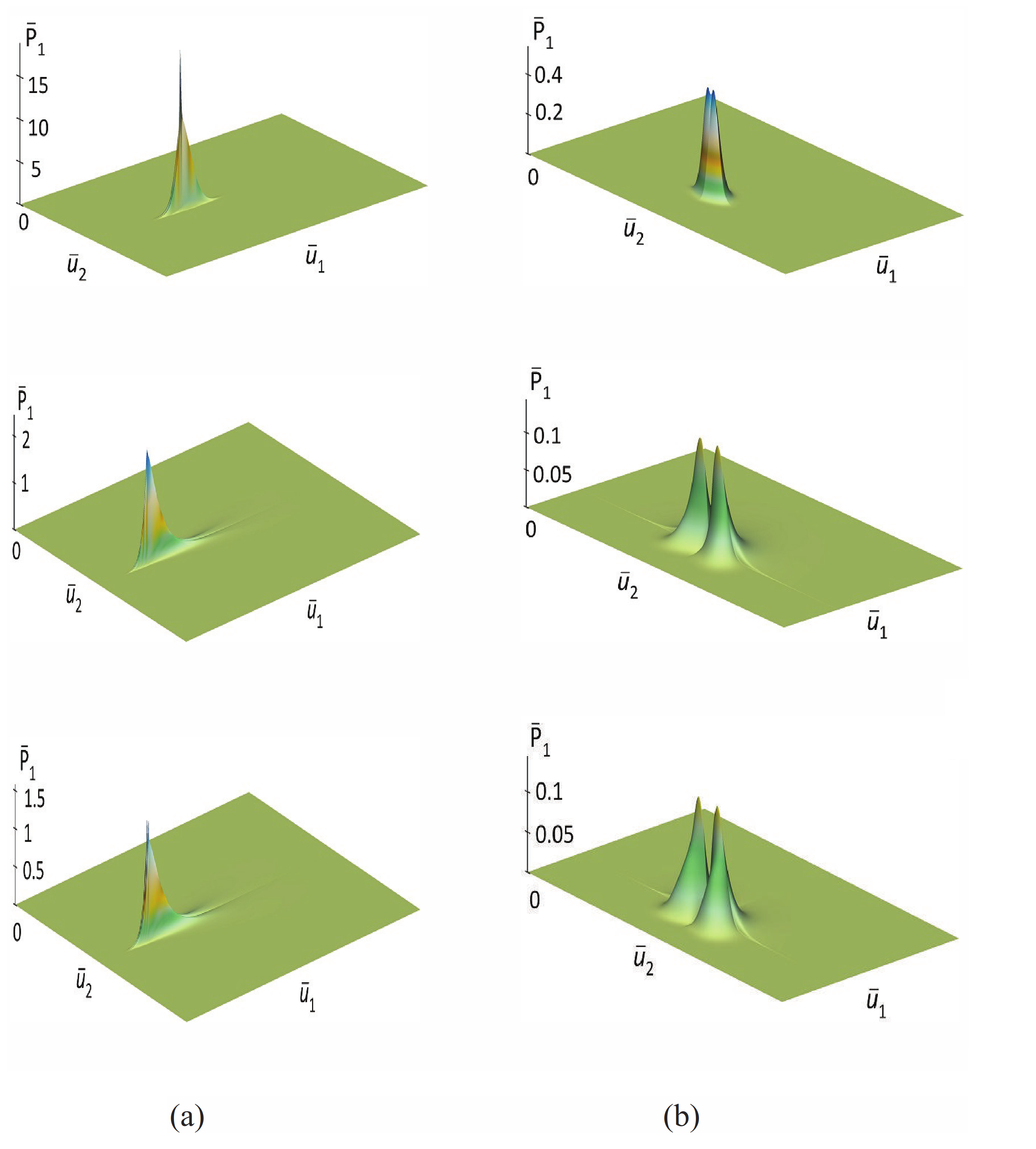
Recall that the data in Table 1 correspond to two coupled 1D linear oscillators immersed in a vacuum with fluctuations, conditionally called a quantum vacuum, and Table 2 shows the initial data describing coupled oscillators in a medium at a finite temperature. For clarity, we considered Equation (43) for a 1D oscillator depending on time, when λ = ( 0.001 , 2.5 ) , ν = 10 and l = 1 (see the first lines of Table 1 and Table 2), i.e., the distribution P ¯ 1 is specifically calculated. We used difference Equation (47), which for ϰ = 4 u ¯ 1 approximates Equation (43) on a discrete lattice and performed calculations based on the data in Table 1 and Table 2.
As can be seen from the comparison of the images of the (a) and (b) columns (see Figure 2), the larger the parameter λ , the more intense relaxation occurs and, accordingly, the faster a small classical environment is formed.

5. Definition of Thermodynamic Potentials and Mean Values of Statistical Parameters

To study irreversible processes in quantum systems, the representation of a non-stationary density matrix developed in the framework of the Liouville–von Neumann equation is often used [37]. However, there is an important limitation associated with the application of this representation, which in number of cases can strongly distort the described phenomena and expected results. It is important to note that the developed representation will be consistent and rigorous if it takes into account both the environmental impact on QS and the QS impact on the environment. As noted above, this can lead to the formation of the so-called small environment, which will have interesting physical properties and have a specific geometric and topological features. Unfortunately, both the standard representation for the density matrix and many modern approaches describing relaxation processes occurring in open systems do not allow achievement the specified rigor of description. To eliminate this flaw in the theory, we propose a new approach, the stochastic density matrix method, which allows us to describe a JS, taking into account the self-consistency between its parts. In other words, we consider and study JS as a closed system that is impossible to implement within the framework of other approaches.
Definition 1.
Let the stochastic density matrix be defined as a bilinear form:
ϱ s t c ( q , t ; { ξ } | q , t ; { ξ } ) = n w n ϱ s t c ( n ) ( q , t ; { ξ } | q , t ; { ξ } ) ,
where ϱ s t c ( n ) = Ψ s t c ( n | q , t ; { ξ } ) Ψ s t c ( n | q , t ; { ξ } ) ; in addition, w n = w n 1 , n 2 = w n 1 ( 1 ) w n 2 ( 2 ) denotes the initial population of the levels of two noninteracting quantum harmonic oscillators that, in the ( i n ) asymptotic state, respectively, possess energies:
E n 1 = ( n 1 + 1 / 2 ) Ω 1 a n d E n 2 = ( n 2 + 1 / 2 ) Ω 2 .
It is important to note that when integrating over the extended space Ξ , the order of integration is important. In particular, if we first integrate stochastic density matrix over the Euclidean space R 2 and then over the functional space R { ξ } , we obtain:
n 1 , n 2 = 0 w n 1 , n 2 = 1 , 0 w n 1 , n 2 1 .
Note that expression (50) is actually a condition for normalizing population levels. It also means that the conservation laws are satisfied on the extended space Ξ .
In the case when the integration is carried out in reverse order, that is, first by the functional space, and then on the Euclidean space, we obtain:
n w n ϱ ¯ n ( T 1 , T 2 ) = 1 , ϱ ¯ n ( T 1 , T 2 ) ) 1 ,
where ϱ ¯ n ( T 1 , T 2 ) = T r q T r { ξ } ϱ s t c ( n ) ( q , t ; { ξ } | q , t ; { ξ } ) denotes the population of the corresponding quantum levels at temperatures of environment T 1 and T 2 ; in addition, T r { ξ } and T r q denote integration operations over functional and Euclidean spaces, respectively (see below (53) and (54)).
The latter means that the conservation laws in the space R 2 as a whole are violated, and only in the limit of statistical equilibrium can we speak about the preservation of their mean values.
Now we will define the mathematical expectation of various random variables.
Definition 2.
The reduced density matrix is defined as the mean value of the random density matrix:
ϱ ( q , t | q , t ) = E ϱ s t c = T r { ξ } ϱ s t c ( q , t ; { ξ } | q , t ; { ξ } ) ,
where E denotes the mathematical expectation of a random variable, and T r { ξ } denotes the functional integration over the environmental fields (see in detail [24]):
T r { ξ } K ( q , t ; { ξ } | q , t ; { ξ } ) = K ( q , t ; { ξ } | q , t ; { ξ } ) D { ξ } .
Definition 3.
The average value of the eigenvalue of the operator A ^ ( q , t ; { ξ } | q , t ; { ξ } ) in the quantum state defined by numbers n = ( n 1 , n 2 ) is written as:
A n = lim t + N n 1 ( t ) T r q T r { ξ } A ^ ϱ s t c ( n ) ,
where N n ( t ) = T r q T r { ξ } ϱ s t c ( n ) ( q , t ; { ξ } | q , t ; { ξ } ) , in addition:
T r q K ( q , t ; { ξ } | q , t ; { ξ } ) = K ( q , t ; { ξ } | q , t ; { ξ } ) d q , d q = d q 1 d q 2 .
As is known, entropy characterizes the measure of randomness of a statistical ensemble, which can be used to find all thermodynamic potentials of the ensemble.
Definition 4.
The von Neumann entropy of a quantum system is determined as [37]:
Λ N ( t ) = T r q ϱ ( q , q , t ) ln ϱ ( q , q , t ) ,
where ϱ ( q , q , t ) ϱ ( q , t | q , t ) | t = t denotes the reduced density matrix.
Definition 5.
The entropy of a quantum subsystem interacting with a random environment can be defined as follows:
Λ G ( t ) = T r q T r { ξ } [ ϱ s t c ( q , t ; { ξ } | q , t ; { ξ } ) ln ϱ s t c ( q , t ; { ξ } | q , t ; { ξ } ) ] .
Obviously, the definition of entropy (57) is rigorous and more consistent and will differ from the value of von Neumann’s entropy when QS interacts strongly with the environment.
Finally, consider the question of the nature of the developed representation from the point of view of fundamental quantum mechanics. As is known, standard quantum mechanics is Hermitian, an important feature of which occurs in the following equalities [38]:
Ψ | H ^ Φ = H ^ Ψ | Φ = H ^ Ψ | Φ ¯ ,
where Ψ and Φ are eigenfunctions of the operator H ^ , in addition, · -scalar product of functions by Dirac’s notation, and · ¯ denotes its complex conjugation. The peculiarity of the developed approach is that the functions Ψ = Ψ s t c ( n | q , t , { ξ } ) L 2 ( Ξ ) and Φ = Ψ s t c ( m | q , t , { ξ } ) L 2 ( Ξ ) are defined in the extended space Ξ R 2 R { ξ } . The latter means that, in the case under consideration, · denotes two types of integration: over the configuration space R 2 and over the function space R { ξ } . From a physical point of view, the integration will make sense if its state will tend to a statistical equilibrium. Based on the above, it is obvious that first of all we must perform integration over the functional space, since this procedure takes into account the JS self-organizing processes. If we assume that the wave functions in (58) are different, then the values of the functional integrals in Ψ | H ^ Φ and H ^ Ψ | Φ will be different and, accordingly, all equalities in (58) will be violated. In other words, the evolution operator (2) is not Hermitian and, accordingly, the developed quantum representation is also non-Hermitian. It is important to note that a direct consequence of the non-Hermitian quantum mechanics is the violation of the detailed balance of transitions between two quantum levels, as well as spontaneous transitions in QS (see Section 10 below).

6. Formation of a Quantized Small Environment under the Influence of QS

Let us consider the evolution of the probability density of a specific quantum state of two coupled 1 D linear oscillators in a random environment. We will assume that all the initial populations of the energy levels, except for one w n = w n 1 n 2 = w n 1 w n 2 0 , are equal to zero. In this case the stochastic density matrix (49) can be represented in the form:
ϱ s t c ( n ) ( q , q , t ; { ξ } ) = l = 1 2 ϱ s t c ( n l ) ( q l , q l , t ; { ξ l } ) ,
where ϱ s t c ( n l ) q l , q l , t ; { ξ l } denotes the random probability density of the 1 D oscillator. Its explicit representation is as follows:
ϱ s t c ( n l ) q l , q l , t ; { ξ l } = g l 2 n l n l ! exp i u 1 ( t ) 2 q l 2 q l 2 u 2 ( t ) 2 q l 2 + q l 2 0 t u 1 ( t ) d t ×
× H n l 2 Ω l exp 0 t u 1 ( t ) d t q l .
Taking into account the probability distribution of free classical environmental fields (26) and (27), we can construct a continuous measure of the functional space R { ξ } (see [24]) and, accordingly, write a functional integral representation for the mathematical expectation of the elements of the density matrix E ϱ s t c ( n ) (see in detail (52) and (53)). Furthermore, using the generalized Feynman–Kac theorem [24], we can calculate the functional integral and reduce it to a double integral representation. In particular, calculating the elements of the density matrix for the first three quantum levels of the 1 D oscillator, we obtain:
ϱ ( 0 ) q l , q l , t = g l + d u 1 0 Q l ( 0 ) ( u 1 , u 2 , t ) exp A l u 1 , u 2 | q l , q l d u 2 , ϱ ( 1 ) q l , q l , t = 2 g l Ω l q l 2 + d u 1 0 Q l ( 1 ) ( u 1 , u 2 , t ) exp A l u 1 , u 2 | q l , q l d u 2 , ϱ ( 2 ) q l , q l , t = ( g l / 2 ) + d u 1 0 Q l ( 0 ) ( u 1 , u 2 , t ) exp A l u 1 , u 2 | q l , q l d u 2 2 g l Ω l q l 2 + d u 1 0 Q l ( 1 ) ( u 1 , u 2 , t ) exp A l u 1 , u 2 | q l , q l d u 2 + 2 g l ( Ω l q l 2 ) 2 + d u 1 0 Q l ( 2 ) ( u 1 , u 2 , t ) exp A l u 1 , u 2 | q l , q l d u 2 ,
where
A l u 1 , u 2 | q l , q l = i u 1 2 q l 2 q l 2 u 2 2 q l 2 + q l 2 .
In addition, the function Q l ( n ) ( u 1 , u 2 , t ) is a solution to the following second-order PDE:
t Q l ( n ) = L ^ l Ω 0 l ( t ) , ϵ l | u 1 , u 2 , t ( 2 n + 1 ) u 1 Q l ( n ) , n = 0 , 1 , 2 , .
Recall that this equation satisfies the Neumann initial-boundary conditions (see (29)). Because the solution Q l ( n ) ( u 1 , u 2 , t ) has the meaning of a probability density, it should be normalized to unity.
Now consider the Equation (61). As we can see, it depends on the vibrational quantum number n of the one-dimensional quantum oscillator, and therefore it can be interpreted as an equation describing the probability distribution of the quantized fields of the environment. In other words, the quantum system extracts a small region from TB and quantizes it. Below, we will call this formation a small quantized environment (SQE).
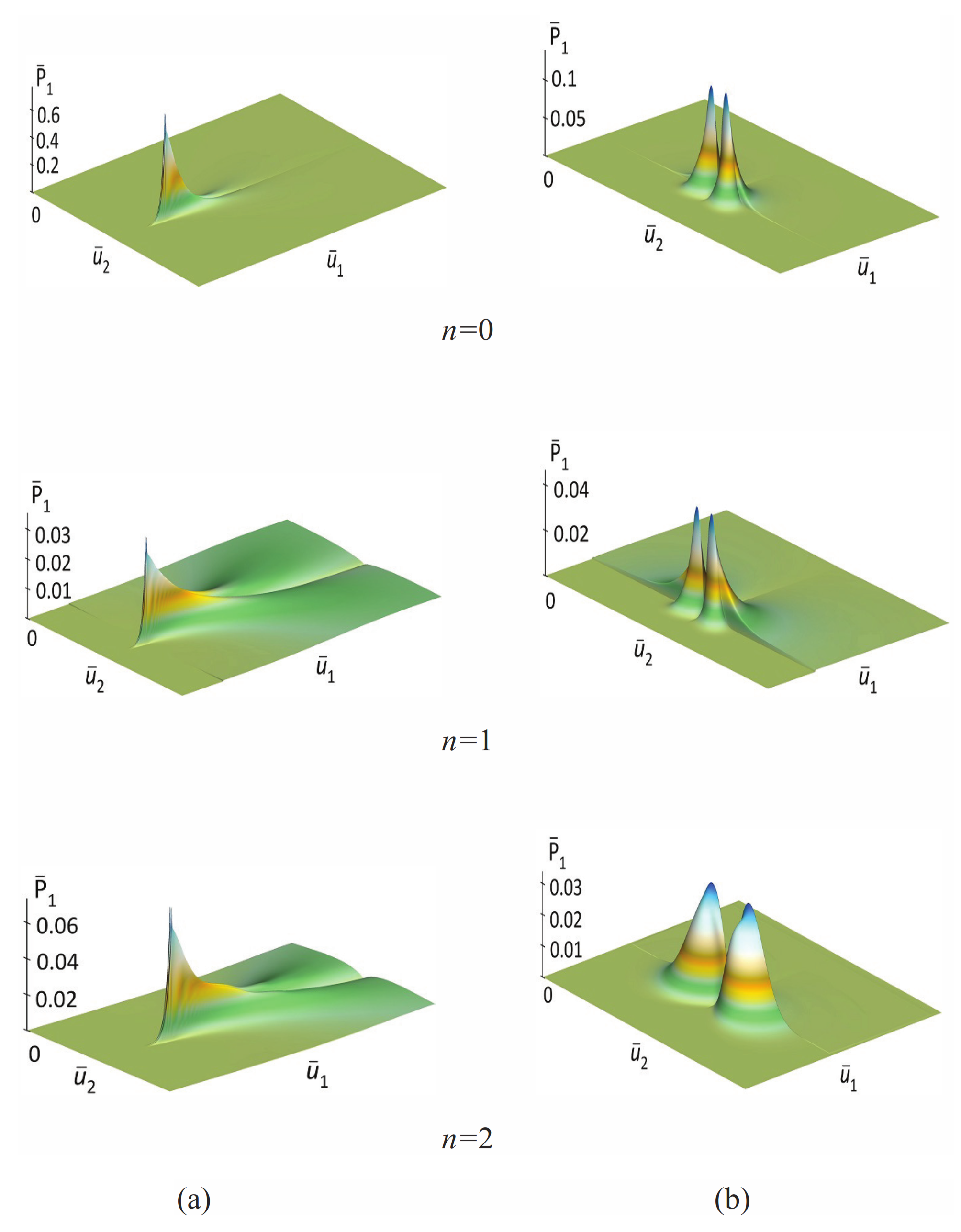
To model these quantum formations, we used the difference Equation (47), which for ϰ = 4 ( 2 n + 1 ) u ¯ 1 , where n = 0 , 1 , 2 , . . approximates the quantum equation of the environment (61) and the data of Table 1 and Table 2. The Equation (47), as in the case of fields of a free environment, is solved as an initial-boundary value problem of Neumann.
Using the first rows of Table 1 and Table 2, we calculated and constructed a series of images showing the probability density of quantized environmental fields at time t = 2 ps (see Figure 3). Note, as numerical calculations show, these distributions are practically close to the limits of their statistical equilibrium. In particular, we see that starting from the quantum number n = 2 , the nature of the solution of Equation (61) changes significantly, which is clearly seen from the images of the field distributions (see the last images in the (a) and (b) columns).
With the elements of the reduced density matrix of the 1D quantum oscillator, we can construct the reduced density matrix of the coupled 2D oscillator. In addition, using expressions (60), we can construct the various probability distributions of 2D oscillator:
ρ ( 00 ) q 1 , q 2 , t , ρ ( 01 ) q 1 , q 2 , t , ρ ( 10 ) q 1 , q 2 , t , ρ ( 11 ) q 1 , q 2 , t ,
where ρ ( n ) q 1 , q 2 , t = ϱ ( n ) q , q , t | q = q , in addition, n = ( n 1 , n 2 ) and q = ( q 1 , q 2 ) .
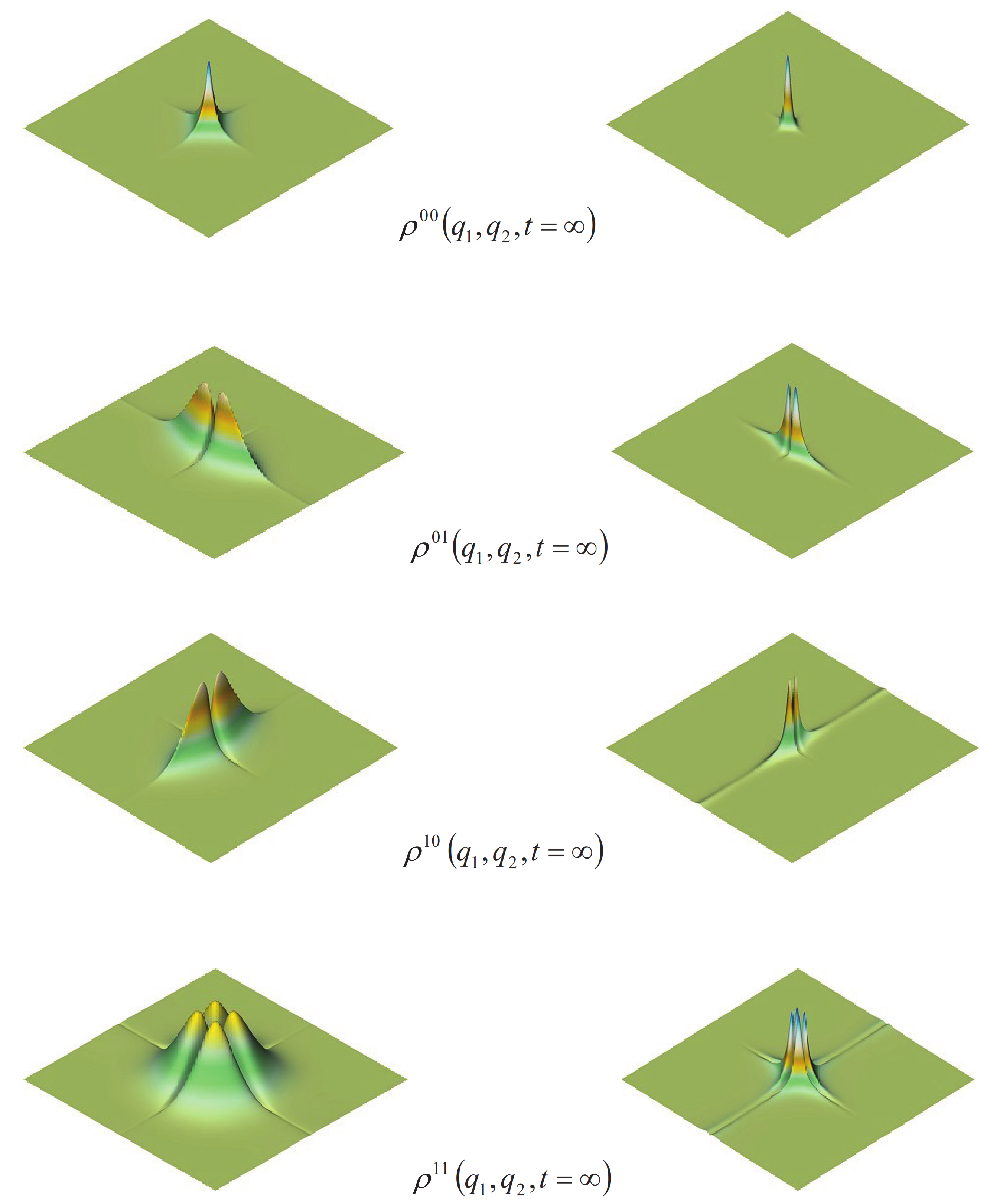
Using the data in Table 1 and Table 2, we calculated quantum distributions for various states (62) without scaling, when t = 10 ps, i.e., when all quantum distributions tend to their statistical equilibrium states (see Figure 4). As we can see in the pictures, the quantum distributions ρ ( 01 ) q 1 , q 2 , t and ρ ( 10 ) q 1 , q 2 , t are very similar; however, they are different and the degree of difference increases with decreasing ν . Recall that the left column contains snapshots of the corresponding quantum distributions of coupled 1 D oscillators in a quantum vacuum, and the right column contains snapshots of these quantum distributions in a medium depending on the temperature, which is determined by the λ parameter.

7. Entropy of the Ground State

Below we consider the features of relaxation immersed in a random environment of a QS. In this sense, the study of the behavior of the entropy of the QS as a function of time can be very important and informative. In this section, we will define the entropy of QS in two different ways.

7.1. The Von Neumann Entropy

Let us consider the reduced density matrix of coupled oscillators in the ground state:
ϱ ( 0 , 0 ) q , q , t = l = 1 2 ϱ ( 0 ) q l , q , t .
To construct the von Neumann entropy, we must substitute (63) into the definition (56) and calculate the trace of an integral:
Λ N ( t ) = N 1 ( 0 ) ( t ) Λ ( 2 ) N ( t ) N 2 ( 0 ) ( t ) Λ ( 1 ) N ( t ) ,
where the following notations are made:
N l ( 0 ) ( t ) = ( Ω l ) 1 / 2 + d u 1 0 Q l ( 0 ) ( u 1 , u 2 , t ) d u 2 u 2 ,
and, respectively,
Λ ( l ) N ( t ) = + ρ ( 0 ) ( q l , t ) ln ρ ( 0 ) ( q l , t ) d q l .
As for the function ρ ( 0 ) ( q l , t ) , then it has to be the following form:
ρ ( 0 ) ( q l , t ) = + d u 1 0 Q l ( 0 ) ( u 1 , u 2 , t ) exp u 2 q l 2 d u 2 .
Since the integration over the coordinate q l in the expression for the function ϱ ( 0 ) ( q l , t ) cannot be performed analytically, further study of the properties of the von Neumann entropy Λ N ( t ) can be realized numerically.

7.2. Entropy of a Quantum State Taking into Account Self-Organization of a JS

Now we can calculate the expectation value of the entropy according to the definition (57). Substituting (63) into expression (57) and performing simple calculations, we obtain the following expression (see [4]):
Λ G ( 0 , 0 ) ( t ) = N 1 ( 0 ) ( t ) Λ ( 2 ) ( 0 ) ( t ) N 2 ( 0 ) ( t ) Λ ( 1 ) ( 0 ) ( t ) ,
where
Λ ( l ) ( 0 ) ( t ) = ( Ω l ) 1 / 2 + d u 1 0 D l ( u 1 , u 2 , t ) d u 2 u 2 .
Notice that the function D l ( λ l , u 1 , u 2 , t ) is a solution of the equation:
t D l = L ^ l D l u 1 Q l ( 0 ) .
Recall that to solve the Equation (67) it is necessary to use the Neumann initial-boundary conditions. It is obvious that in the limit of thermodynamic equilibrium the entropy should move towards the stationary limit:
Λ G ( 0 , 0 ) ( ϵ ¯ l ) = lim t + Λ G ( 0 , 0 ) ( t ) , ϵ ¯ l = ( ϵ ¯ 1 , ϵ ¯ 2 ) .
If we assume that in the limit t + the interaction between two coupled 1 D oscillators vanishes, i.e., when ω 0 , then ϵ ¯ 1 = ϵ ¯ 2 . However, this does not mean at all that the parameters N 1 ( 0 ) with N 2 ( 0 ) and Λ 1 with Λ 2 in this case coincide. Moreover, as follows from the expression (60), if these oscillators have ever interacted, then the specified parameters will obviously not be the same.
To summarize, note that in both definitions of entropy (64) and (66), the entanglement of the states of two separate 1D oscillators is obvious. In addition, it is necessary to note that when the parameter ϵ ¯ l = ( ϵ ¯ 1 , ϵ ¯ 2 ) 0 , then the functions N 1 ( 0 ) ( t ) and N 2 ( 0 ) ( t ) tend towards unity and, accordingly, the entropy of separate oscillators of the QS as a whole should tend towards zero, which will satisfy the condition that the environment is switching off.

8. Energy Levels and Their Occupancy after Relaxation in TB

The energy spectrum is an important characteristic of a quantum system. Below we will study the energy levels of a 1 D oscillator after switching on the TB and establishing thermodynamic equilibrium in the QS. For the example, we will calculate the first several energy levels. Taking into account (54), it is easy to obtain the mathematical expectations of the energy levels. In particular, for the energy level of the ground state we obtain:
E 0 ( λ l , μ ) = 1 2 1 + K 0 ( λ l , μ ) Ω l + ,
where
K 0 ( λ l , μ ) = + d u ¯ 1 0 1 + 1 + u ¯ 1 2 + u ¯ 2 2 2 u ¯ 2 d l Q ˜ l ( 0 ) ( λ l , μ ; u ¯ 1 , u ¯ 2 ) d u ¯ 2 u ¯ 2 .
Recall that d l = Ω l + / Ω l ; in addition, the distribution function Q ˜ l ( 0 ) is a solution of stationary dimensionless Equation (61), which is formed in the limit t ¯ + . Obviously, in the limit λ l 0 and μ = 0 for the energy level of the ground state we should obtain the result:
lim λ l 0 E 0 ( λ l , 0 ) = 1 2 Ω l + .
The latter, in turn, means that the distribution function Q ˜ l ( 0 ) in this limit should have the following form:
lim λ l 0 Q ˜ l ( 0 ) ( λ l , 0 ; u ¯ 1 , u ¯ 2 ) = δ ( u ¯ 1 ) δ ( u ¯ 2 u ¯ 02 ) ,
where u ¯ 02 = d l ± d l 2 1 .
In the case when d l > 1 , obviously there are two solutions Q ˜ l ( 0 ) and Q ˜ l ( 0 + ) and, therefore, two energy levels characterizing the ground state, which we will denote with E 0 ( λ l , μ ) and E 0 + ( λ l , μ ) , respectively.
Similarly, we can calculate the mathematical expectation of the energy level of the first excited state:
E 1 ( λ l , μ ) = 3 2 1 + K 1 ( λ l , μ ) Ω l + ,
where
K 1 ( λ l , μ ) = + d u ¯ 1 0 1 + 1 + u ¯ 1 2 + u ¯ 2 2 2 u ¯ 2 d l Q ˜ l ( 2 ) ( λ l , μ ; u ¯ 1 , u ¯ 2 ) d u ¯ 2 u ¯ 2 u ¯ 2 .
It is easy to verify that when d l > 1 , in this case also the energy level is split into two sub-levels E 1 ( λ l , μ ) and E 1 + ( λ l , μ ) , respectively. Note that even in the case d l = 1 , when all the sublevels disappear or, more precisely, merge, the spectrum of the quantum oscillator in the case under consideration is fundamentally different from the spectrum of an oscillator without an environment. In particular, the equidistance between energy levels is violated in this case.
Finally, in the limit of statistical equilibrium, we can calculate the populations of different quantum levels as a function of temperature:
M n ( λ l , μ ) = T r q l T r ξ l ϱ ( n ) ( q l , t ; { ξ l } | q l , t ; { ξ l } ) .
In particular, using the previous formula for the ground state population level, we find the following expression:
N l ( 0 ) ( t ) = M 0 ( λ l , μ ) = + d u ¯ 1 0 Q l ( 0 ) ( λ l , μ ; u ¯ 1 , u ¯ 2 ) d u ¯ 2 u ¯ 2 ,
and for the first excited state, respectively:
M 1 ( λ l , μ ) = + d u ¯ 1 0 Q l ( 2 ) ( λ l , μ ; u ¯ 1 , u ¯ 2 ) d u ¯ 2 u ¯ 2 u ¯ 2 .

9. Quantum Entanglement of States Caused by Random Environment

Performing coordinate transformations (3), the original problem of coupled oscillators is reduced to the problem of two noninteracting oscillators in a random environment. Let the numbers one and two, as indicated above, denote noninteracting oscillators in a random environment whose wave states in the Hilbert spaces H 1 ( R 1 R ξ 1 ) and H 2 ( R 1 R ξ 2 ) are denoted by the functions Ψ s t c ( 1 ) L 2 ( R 1 R ξ 1 ) and Ψ s t c ( 2 ) L 2 ( R 1 R ξ 2 ) , respectively.
The Hilbert space of the composite system is the tensor product H = H 1 H 2 , while the state of the composite system is defined as:
Ψ s t c ( 1 ) Ψ s t c ( 2 ) = n c n 1 | n 1 m c m 2 | m 2 H .
In (74) the vectors | n 1 = Y s t c ( 1 ) ( n | q 1 , t ; { ξ 1 } ) and | m 2 = Y s t c ( 2 ) ( m | q 2 , t ; { ξ 2 } ) denote the exact states of 1 D quantum oscillators in the random environment (see expression (11)), in addition, c n 1 and c m 2 are some complex numbers with absolute values, | c n 1 | , | c m 2 | 1 . Obviously, each set of functions { | n 1 } and { | m 2 } forms an orthonormal basis in the Hilbert spaces H 1 and H 2 , respectively.
If the numbers c n 1 and c m 2 are not equal to zero, then in general the separable states can be represented as a direct product:
Ψ J S = n , m c n m | n 1 | m 2 , c n m = n n 1 c m 2 .
where Ψ J S denotes the wave function of JS.
Based on the properties (1)–(16), it is easy to show that in the extended space Ξ R 2 R { ξ } the wave state Ψ J S is separable. However, a reasonable question arises: what happens if the wave function Ψ J S is averaged over the functional space R { ξ } ? Obviously, from a physical point of view, this would mean calculating the mathematical expectation of the wave function of coupled quantum oscillators taking into account the influence of a random environment:
Ψ ¯ Q S ( q , t ) = E [ Ψ J S ] = n , m c n m | n ¯ 1 | m ¯ 2 , n , m = 0 , 1 , 2 ,
where Ψ ¯ Q S = E [ Ψ J S ] = Ψ J S R { ξ } denotes the functional integration over the space R { ξ } .
For definiteness, consider the case c n m = 0 for n + m 1 , i.e., when both oscillators are in ground states or one of them is in the ground state, and the other is in the first excited state. In this case, from (76) for the wave function of QS we obtain the following expression:
Ψ ¯ Q S ( q , t | 0 , 0 ) = | 0 ¯ 1 | 0 ¯ 2 ,
where
| 0 ¯ l = ( g l ) 1 / 2 + d u 1 0 Υ l ( 1 2 , 1 2 ) ( u 1 , u 2 , t ) exp 1 2 i u 1 u 2 q l 2 d u 2 ,
describes the l-th oscillator ground state entangled with the environment. As for the complex function Υ l ( 1 2 , 1 2 ) ( u 1 , u 2 , t ) , it satisfies the following PDE:
t Υ l ( p , k ) = L ^ l ( p u 1 + i k u 2 ) Υ l ( p , k ) ,
for the case p , k = 1 / 2 .
Obviously, the complex function Υ l ( p , k ) ( u 1 , u 2 , t ) cannot have the meaning of a probability density. Rather, it can be interpreted as a wave function of forming the small environment that is closely related or, more accurately, entangled with QS. In other words, the SE under the influence of QS is quantized and therefore the value | Υ l ( p , k ) ( u 1 , u 2 , t ) | 2 should be interpreted as a probability distribution of SE corresponding to the certain quantum state of the QS. It is easy to show that for any values ( p , k ) ( 0 , ) the integral:
| C l ( p , k ; t ) | 2 = + d u 1 0 | Υ l ( p , k ) ( u 1 , u 2 , t ) | 2 d u 2 < ,
and therefore the function Υ ¯ l ( p , k ) ( u 1 , u 2 , t ) can be normalized to unity.
The Equation (79) can be represented as a system of two real equations:
{ t R l ( p , k ) = L ^ l R l ( p , k ) p u 1 R l ( p , k ) k u 2 I l ( p , k ) , t I l ( p , k ) = L ^ l I l ( p , k ) p u 1 I l ( p , k ) + k u 2 R l ( p , k ) ,
where Υ l ( p , k ) ( u 1 , u 2 , t ) = R l ( p , k ) ( u 1 , u 2 , t ) + i I l ( p , k ) ( u 1 , u 2 , t ) .
It is easy to see that the system of Equation (81) is symmetric with respect to permutations R l ( p , k ) I l ( p , k ) and I l ( p , k ) R l ( p , k ) . On the other hand, this means that these solutions transit to each other as a result of coordinate transformations. In particular, we can establish the following general properties, which these solutions should possess:
R l ( p , k ) ( u 1 , u 2 , t ) = I l ( p , k ) ( u 1 , u 2 , t ) = I l ( p , k ) ( u 1 , u 2 , t ) , I l ( p , k ) ( u 1 , u 2 , t ) = R l ( p , k ) ( u 1 , u 2 , t ) = R l ( p , k ) ( u 1 , u 2 , t ) .
Given the properties (80), we can separate the equations by writing them in a mutually independent form:
t R l ( p , k ) = L ^ l R l ( p , k ) p u 1 + k u 2 R l ( p , k ) , t I l ( p , k ) = L ^ l I l ( p , k ) p u 1 k u 2 I l ( p , k ) .
To solve each of these partial differential equations, one can use initial and boundary conditions of the type (28) or (29).
For quantum communications, entangled states consisting of various vector states are of particular interest. In particular, we can construct a quantum gate with the following four Bell states:
Ψ J S = 1 2 | 0 1 | 0 2 | 1 1 | 1 2 , Φ J S = 1 2 | 0 1 | 1 2 | 1 1 | 0 2 .
By performing functional integration over these states, we obtain mathematical expectations for the following entangled Bell states:
Ψ ¯ Q S ( q 1 , q 2 , t ) = E Ψ J S = 1 2 | 0 ¯ 1 | 0 ¯ 2 | 1 ¯ 1 | 1 ¯ 2 , Φ ¯ Q S ( q 1 , q 2 , t ) = E Φ J S = 1 2 | 0 ¯ 1 | 1 ¯ 2 | 1 ¯ 1 | 0 ¯ 2 ,
where Ψ ¯ Q S ( q 1 , q 2 , t ) = Ψ J S R { ξ } and Φ ¯ Q S ( q 1 , q 2 , t ) = Φ J S R { ξ } , in addition:
| 1 ¯ l = 2 ( g l ) 1 / 2 q l + d u 1 0 Υ ¯ l ( 3 2 , 3 2 ) ( u 1 , u 2 , t ) exp 1 2 i u 1 u 2 q l 2 d u 2 .
Recall that the wave function Υ ¯ l ( 3 2 , 3 2 ) ( u 1 , u 2 , t ) is a solution of Equation (79) for the case p , k = 3 / 2 , which is normalized to unity.
Note that the states (84) differ from ordinary Bell states in that their constructions include nonorthogonal basis functions of the corresponding Hilbert spaces as a result of additional integration over TB:
| 0 ¯ 1 , | 1 ¯ 1 H ¯ 1 ( 1 ) ( R 1 ) = H 1 ( R 1 R ξ 1 ) R ξ 1 ,
and, correspondingly,
| 0 ¯ 2 , | 1 ¯ 2 H ¯ 1 ( 2 ) ( R 1 ) = H 2 ( R 1 R ξ 2 ) R ξ 2 .
Note that an important feature of the developed representation is the presence of a number of parameters that allow organization of effective external control over the QS.

10. Transitions Probabilities between Different Asymptotic Quantum States

Let us consider the evolution of the QS under the influence of a random environment, taking into account possible quantum transitions. Let the fluctuations in the environment continue for a finite time. We assume that, in the time interval t ( t 0 , t 0 ] , the random force f l ( t ) acts on QS, and on the time interval t [ t 0 , + ) this influence disappears, i.e., f l ( t ) 0 . It follows from the above that in the t + limit the wave function Ψ o u t ( m | q , t ) has the form:
Ψ s t c ( n | q , t ; { ξ } ) = m C n m ( t ; { ξ } ) Ψ o u t ( m | q , t ) ,
where Ψ o u t ( m | q , t ) is the stationary wave function QS in the asymptotic state ( o u t ) , which describes the quantum state of coupled oscillators for times t > t 0 , which can be represented as follows:
Ψ o u t ( m | q , t ) = l = 1 2 e i ( m l + 1 / 2 ) Ω l + t ϕ m l ( q l ) ,
where
ϕ m l ( q l ) = g l + 2 m l m l ! 1 / 2 e ( Ω l + q l 2 ) / 2 H m l Ω l + q l , g l + = ( Ω l + / π ) 1 / 2 .
Definition 6.
The mathematical expectation of the probability of transition between the asymptotic channels ( i n ) and ( o u t ) will be determined by the following formula:
W n m = lim t + E S nm ( q , t ; { ξ } ) 2 = lim t + T r { ξ } T r q S nm ( q , t ; { ξ } ) 2 ,
where S nm ( q , t ; { ξ } ) = Ψ s t c ( n | q , t ; { ξ } ) Ψ o u t ( m | q , t ) denotes a random S -matrix element.
To perform analytical calculations, we can use the generating functions method, but now for random processes (see [23]):
Ψ s t c ( α | q , t ; { ξ } ) = l = 1 2 n l = 0 α n l n l ! Y s t c ( n l | q l , t ; { ξ l } ) ,
and
Ψ o u t ( β | q , t ) = l = 1 2 m l = 0 β m l m l ! e i ( m l + 1 / 2 ) Ω l + t ϕ m l ( q l ) ,
where α = ( α 1 , α 2 ) and β = ( β 1 , β 2 ) are auxiliary complex variables.
Calculating the sum in the representation (89) leads to an expression that is the product of two Gaussian wave packets:
Ψ s t c ( α | q , t ; { ξ } ) = l = 1 2 ( g l ) 1 / 2 exp 1 2 a l q l 2 2 b l q l + c l ,
where a l , b l and c l are random variables, which are defined by the following expressions:
a l = i ξ l ˙ ξ l 1 , b l = 2 Ω l α l ξ l 1 , c l = ξ l ξ l 1 α l 2 + ln ξ l .
It is easy to see that the random wave packet (91) in the ( i n ) asymptotic state transits a determined quantum state:
Ψ s t c ( α | q , t ; { ξ } ) | t = Ψ i n ( α | q , t ) = l = 1 2 ( g l ) 1 / 2 exp 1 2 Ω l q l 2 2 2 Ω l α l q l e i Ω l t + α l 2 e i 2 Ω l t + i Ω l t .
Obviously, the generating function Ψ o u t ( β | q , t ) can be easily found from the expression (93) by making the following substitutions Ω l Ω l + and α l β l .
Now we consider the following integral:
J s t c ( α , β | t ; { ξ } ) = Ψ s t c ( α | q , t ; { ξ } ) Ψ o u t ( β | q , t ) d q .
Performing simple calculations, we obtain:
J s t c ( α , β | t ; { ξ } ) = l = 1 2 ( Ω l Ω l + ) 1 / 4 a ¯ l exp b ¯ l 2 4 a ¯ l c ¯ l ,
where the following notations are used:
a ¯ l = 1 2 a l + Ω l + , b ¯ l = b l + 2 Ω l + β l e i Ω l + t , c ¯ l = 1 2 c l + β l 2 e i 2 Ω l + t i Ω l + t .
For further calculations, it is useful to represent the generating function (95) as the following decomposition:
J s t c ( α , β | t ; { ξ } ) = l = 1 2 n l , m l = 0 α l n l n l ! C n l m l l ( t ; { ξ l } ) β l m l m l ! , C n m = l = 1 2 C n l m l l ,
from which it follows, that:
l = 1 2 C n l m l l ( t , { ξ l } ) = l = 1 2 1 n l ! m l ! n l + m l α l n l β l m l J s t c ( α , β | t ; { ξ } ) | α l = β l = 0 .
Using (95) and (96), we can write the transition probability in the following form:
W n m = lim t + l = 1 2 T r { ξ l } C n l m l l ( t ; { ξ l } ) 2 .
It is easy to verify that the transition probability (97) formally is a product of the transitions probabilities of two 1 D oscillators. In other words, we can represent the Equation (97) in a factored form:
W n m = l = 1 2 w n l m l ( l ) , W n l m l ( l ) = lim t + T r { ξ l } C n l m l l ( t ; { ξ l } ) 2 .
Thus, by calculating the transition probabilities of 1 D quantum oscillator, we can construct the corresponding transitions of 2D oscillator.
As an example, let us calculate a series of transition probabilities between ( i n ) and ( o u t ) asymptotic channels. Taking into account (92), (95) and (97), we can construct explicit form of the functional integral and calculate it using the generalized Feynman–Kac theorem (see [24]). In particular, for the transition probability between the ground states of the ( i n ) and ( o u t ) asymptotic channels, we obtain the following integral representation:
W 0 0 ( l ) = κ l + d u ¯ 1 0 + Υ ¯ l ( 1 2 , 1 2 ) ( λ l , μ ; u ¯ 1 , u ¯ 2 ) ( 1 + u ¯ 2 i u ¯ 1 ) 1 2 d u ¯ 2 2 ,
where the following notations are used:
λ l = ϵ ¯ l / ( Ω l + ) 3 , κ l = 2 ( Ω l / Ω l + ) 1 / 2 , u ¯ 1 = u 1 / Ω l + , u ¯ 2 = u 2 / Ω l + .
As for the stationary wave function Υ ¯ l ( 1 2 , 1 2 ) ( λ l , u ¯ 1 , u ¯ 2 ) , then it is the solution of the Equation (79) in the limit t ¯ + , which in the dimensionless form is written as:
t ¯ Υ ¯ l ( p , k ) = L ^ ¯ l ( p u ¯ 1 + i k u ¯ 2 ) Υ ¯ l ( p , k ) , t ¯ = Ω l + t ,
where
L ^ ¯ l = λ l 2 u ¯ 1 2 + μ 2 u ¯ 2 2 + u ¯ 1 u ¯ 1 2 u ¯ 2 2 + Ω ¯ 0 l 2 ( t ) + 2 u ¯ 1 u ¯ 2 u ¯ 2 , Ω ¯ 0 l ( t ) = Ω 0 l ( t ) Ω l + .
Similarly, we can calculate probabilities of other transitions of the 1 D oscillator. In particular the first few transitions can be represented in the form:
W 1 1 ( l ) = κ l 3 + d u ¯ 1 0 Υ ¯ l ( 3 2 , 3 2 ) ( λ l , μ ; u ¯ 1 , u ¯ 2 ) ( 1 + u ¯ 2 i u ¯ 1 ) 3 2 d u ¯ 2 2 , W 0 2 ( l ) = κ l + d u ¯ 1 0 1 u ¯ 2 + i u ¯ 1 ( 1 + u ¯ 2 i u ¯ 1 ) 3 2 Υ ¯ l ( 1 2 , 1 2 ) ( λ l , μ ; u ¯ 1 , u ¯ 2 ) d u ¯ 2 2 , W 2 0 ( l ) = κ l + d u ¯ 1 0 κ l 2 Υ ¯ l ( 2 , 2 ) ( λ l , μ ; u ¯ 1 , u ¯ 2 ) ( 1 + u ¯ 2 i u ¯ 1 ) 3 2 Υ ¯ l ( 2 , 0 ) ( λ l , μ ; u ¯ 1 , u ¯ 2 ) ( 1 + u ¯ 2 i u ¯ 1 ) 1 2 d u ¯ 2 2 ,
where the wave function Υ ¯ l ( p , k ) ( λ l , μ ; u ¯ 1 , u ¯ 2 ) denotes the stationary solution of the Equation (100) in the limit t ¯ + .
In particular, as follows from the expressions of transition probabilities (101), only transitions between states with the same parity are possible. However, the most important and unexpected result is the violation of the detailed balance of transitions between the quantum levels W n m W m n , which is the cornerstone of standard quantum mechanics. In particular, we can verify this by comparing the following two transition amplitudes W 0 2 ( l ) and W 2 0 ( l ) .
Now it is important to show that, when the medium is turned off, the amplitude of the transition probability coincides with the transition amplitude of the parametric oscillator. For the example, let us rewrite the expression for the “ground state-ground state" transition (99) in the form:
W 0 0 ( l ) = κ l + d u ¯ 1 0 1 ϱ ( u ¯ 1 , u ¯ 2 ) 1 / 4 Υ ¯ l ( 1 2 , 1 2 ) ( λ l , μ ; u ¯ 1 , u ¯ 2 ) e i φ ( u ¯ 1 , u ¯ 2 ) d u ¯ 2 ,
where
ϱ ( u ¯ 1 , u ¯ 2 ) = 1 u ¯ 1 2 + u ¯ 2 2 + 2 u ¯ 2 u ¯ 1 2 + ( 1 + u ¯ 2 ) 2 , φ ( u ¯ 1 , u ¯ 2 ) = 1 + u ¯ 2 u ¯ 1 2 + ( 1 + u ¯ 2 ) 2 , 0 ϱ ( u ¯ 1 , u ¯ 2 ) 1 .
To consider to the well-known 1D problem of a parametric oscillator, it is obviously necessary to put μ = 0 and λ l 0 . The latter, in turn, implies that the imaginary part of the solution Υ l ( 1 2 , 1 2 ) is zero and, consequently, it is necessary to replace Υ l ( 1 2 , 1 2 ) R l ( 1 2 , 1 2 ) and, in addition, the stationary solution R l ( 1 2 , 1 2 ) ( λ l , μ ; u ¯ 1 , u ¯ 2 ) must satisfy the condition:
lim λ l 0 R l ( 1 2 , 1 2 ) ( λ l , μ ; u ¯ 1 , u ¯ 2 ) = λ l 1 δ ( u ¯ 1 ) δ ( u ¯ 2 u ¯ 02 ) , u ¯ 02 = 1 + 1 1 ρ ,
where ρ = C 2 ( l ) / C 1 ( l ) 2 .
Recall that the coefficients C 1 ( l ) and C 2 ( l ) are found from the solution of the classical Equation (10) with the regular frequency Ω 0 l ( t ) , in the limit t + . In this case, the classical oscillator goes to the ( o u t ) channel, and the solution takes the form; ξ 0 l ( t ) C 1 ( l ) e i Ω l + t C 2 ( l ) e i Ω l + t .
Finally, substituting (103) into (102), we obtain a well-known result for the transition probability of the 1 D parametric oscillator; W 0 0 ( l ) = 1 ρ . Note that in the same way as for λ l 0 , we can pass to the known regular values (see [23]) for other transitions (101).
It should be noted that the probabilities of 1 D transitions are important for calculating the mathematical expectation of Bell states (see Section 9).

11. Conclusions

The main goal of the study was to develop a representation that allows exploration of the evolution of the "QS + environment (universe)" as a single self-organizing system. To implement this idea, we postulated an equation of the Langevin–Schrödinger type as the basic equation for describing the JS, for which the Schrödinger equation plays the role of the principle of local correspondence. Recall that this is equivalent to the condition when in certain short time intervals, between two random environmental influences, the QS would be described by the Schrödinger equation. It should be noted that precisely constructed models’ QS with a random environment can be very informative and useful for a deeper understanding of the problems of quantum foundations, including for the development of quantum thermodynamics from the first principles of non-Hermitian quantum mechanics.
For a consistent mathematical construction of this problem, we considered the task of two linearly coupled 1D quantum oscillators immersed in a random environment or TB. Recall that this model, despite its apparent simplicity, can describe the basic properties of a quantum reacting molecular gas, which is very important for the development of modern technologies. In addition, within the framework of this model, various questions of quantum optics and quantum communications can be investigated.
We rigorously proved that, within the framework of this model, all statistical parameters of the QS can be mathematically constructed in a closed form using two-dimensional integral representations and second-order PDE solutions. One of the most important results of the research is the proof of the formation of a quantized small environment as a result of JS self-organization processes. Note that the physical meaning of QSE can be interpreted as a continuation of the quantum subsystem or, more precisely, its quantum halo that is entangled with QS and contains information about it.
The paper calculates the time-dependent quantum entropy for two coupled 1D quantum oscillators in the ground state. It is shown that the von Neumann quantum entropy and its generalized version, which takes into account the JS self-organization process (see (66)), are, generally speaking, different. As the analysis shows, both expressions of entropy coincide only when the influence of the environment on QS is negligible. It should be noted that from the expression of generalized entropy (66) it follows that the environment makes the quantum subsystem inseparable. In particular, when QS decays into two independent 1 D oscillators, which are outgoing to infinity, a non-potential interaction arises between them, which is characteristic of entangled quantum states. The considered representation makes it possible to study in detail and deeply the role of the random environment in the entanglement phenomenon of spatially isolated quantum subsystems and suggests possibility of organizing efficient control of the entanglement properties through the parameters of the environment. We expect that a simulation of expressions (78) can give important information on a role of entangling in the process of thermal relaxation of an environment and the degree of violation of the basic principle of statistical physics on the equiprobability of statistical states [21].
The probabilities of transitions between different asymptotic states of a 1D quantum oscillator are calculated explicitly taking into account the influence of TB. In particular, from the expression (101) it follows that W 02 W 20 , i.e., one of the fundamental principle of quantum mechanics, namely, the detailed balance of transitions between two pure states is violated even in vacuum taking into account quantum fluctuations. On the other hand, this result is a direct consequence of the non-Hermitian character of the operator H ^ x , t ; { f } (see expression (2)), which is typical for non-Hermitian quantum mechanics [39,40]. Note that the derivation of expressions for quantum transitions allows one to construct kinetic equations and directly simulate the population of the energy levels of the QS, which is very important for testing the hypothesis of a micro-canonical distribution in a quantum ensemble under thermal equilibrium conditions.
It should be noted that this study may also shed new light on some fundamental problems of the quantum foundations and quantum statistical mechanics. In particular, regarding the possibilities of changing and effectively controlling the fundamental properties of quantum mechanics, such as the Heisenberg uncertainty principles, the energy spectrum of the QS, the properties of entanglement between quantum states, etc. In addition, this study makes it possible to clearly answer the question of the possibility of violating a number of laws of thermodynamics, in particular, the second law of thermodynamics, when quantum fluctuations are taken into account [41,42,43].
Finally, it is fundamentally important to carry out research in order to find a set of external parameters at which it would be possible to significantly violate the detailed equilibrium between the quantum transitions by making W 02 > W 20 . Recall that this would allow us to seriously think about the possibility of extracting energy from the quantum vacuum.

Author Contributions

The concept of a new representation of an open quantum system (QS) using the hidden dynamical symmetry of the internal motion of the QS, which makes it possible to consider the system as closed, was developed by A.S.G. The mathematical algorithm and code for the numerical calculation and vizualization of the problem were developed by A.V.B. and V.V.M. All authors participated in writing and numerous corrections of the article. All authors have read and agreed to the published version of the manuscript.

Funding

This research received no external funding.

Institutional Review Board Statement

The research is carried out within the framework of the basic scientific plans of the institutes where the authors of the article work.

Informed Consent Statement

The decision to publish this article was made by all authors.

Data Availability Statement

References are given in the work, which, in our opinion, quite fully reflect the urgent problems of open quantum systems (OQS). As for our work, it is original, in which fundamentally new physical ideas and mathematical concepts are developed. In particular, the new formulation of OQS makes it possible to avoid the loss of information in JS and for the first time to prove the existence of a new physical object, namely, the formation of a quantized small environment or a quantum halo of a QS.

Conflicts of Interest

The authors declare no conflict of interest.

References

  1. Davtyan, O.K. Theory of Gravitational-Inertial Field of Universe. IV. The Universe and the Microcosm. Ann. Phys. 1979, 36, 227. [Google Scholar] [CrossRef]
  2. Davtyan, O.K.; Karamyan, G.G. Theories of Inertial Field’s and of Quantum Correlations. Acad. Sci. ARM 1987, 137. [Google Scholar]
  3. Milonni, P.W. The Quantum Vacuum: An Introduction to Quantum Electrodynamics. Am. J. Phys. 1994, 62, 1154. [Google Scholar] [CrossRef]
  4. Gevorkyan, A.S. Exactly constructing model of quantum mechanics with random environment. Phys. Atom. Nucl. 2010, 73, 311–319. [Google Scholar] [CrossRef]
  5. Gevorkyan, A.S. Nonrelativistic Quantum Mechanics with Fundamental Environment. Found. Phys. 2011, 41, 509–515. [Google Scholar] [CrossRef] [Green Version]
  6. Gevorkyan, A.S. Quantum Vacuum: The Structure of Empty Space-Time and Quintessence with Gauge Symmetry Group SU(2)xU(1). Particles 2019, 2, 281–308. [Google Scholar] [CrossRef] [Green Version]
  7. Gemmer, J.; Michel, J.M.; Mahler, G. Quantum Thermodynamics: Emergence of Thermodynamic Behavior Within Composite Quantum Systems (Second Edition). In Lecture Notes in Physics; Springer: Heidelberg, Germany, 2009. [Google Scholar]
  8. Borowski, P.; Gemmer, J.; Mahler, G. Relaxation into equilibrium under pure Schrödinger dynamics. Eur. Phys. J. B 2003, 35, 255–259. [Google Scholar] [CrossRef] [Green Version]
  9. Allahverdyan, A.E.; Balian, R.; Nieuwenhuizen, T.M. Understanding quantum measurement from the solution of dynamical models. Phys. Rep. 2013, 525, 1–201. [Google Scholar] [CrossRef] [Green Version]
  10. Davies, E.B. Quantum Theory of Open Systems; Academic Press: London, UK; New York, NY, USA, 1976. [Google Scholar]
  11. Exner, P. Open Quantum Systems and Feynman Integrals; Fundamental Theories of Physics Book Series; Springer: Dordrecht, The Netherlands, 1985; Volume 6. [Google Scholar]
  12. Marquardt, F.; Püttmann, A. Introduction to dissipation and decoherence in quantum systems. arXiv 2008, arXiv:0809.4403v1. [Google Scholar]
  13. Zurek, W.H. Decoherence from spin environments. Rev. Mod. Phys. 2003, 75, 715. [Google Scholar] [CrossRef] [Green Version]
  14. Schlosshauer, M.A. Decoherence and the quantum-to-classical transition. In The Frontiers Series; Springer: Berlin/Heidelberg, Germany, 2007. [Google Scholar]
  15. Zurek, W.H. Decoherence, einselection, and the quantum origins of the classical. Phys. Rev. Lett. 2002, 88, 715. [Google Scholar] [CrossRef] [Green Version]
  16. Joshi, C.; Hutter, A.; Zimmer, F.; Jonson, M.; Andersson, E.; Öhberg, P. Quantum entanglement of nanocantilevers. Phys. Rev. B 2010, 82, 043846. [Google Scholar] [CrossRef] [Green Version]
  17. Dunningham, J.A.; Palge, V.; Vedral, V. Entanglement and nonlocality of a single relativistic particle. Phys. Rev. A 2009, 80, 044302. [Google Scholar] [CrossRef] [Green Version]
  18. Breuer, H.P.; Petruccione, F. The Theory of Open Quantum Systems; Oxford University Press: Oxford, UK, 2002. [Google Scholar]
  19. Lidar, D.A. Lecture Notes on the Theory of Open Quantum Systems. arXiv 2020, arXiv:1902.00967v2. [Google Scholar]
  20. Nielsen, M.A.; Chuang, I.L. Quantum Computation and Quantum Information; Cambridge University Press: New York, NY, USA, 2010; 704p. [Google Scholar]
  21. Popescu, S.; Shor, A.J.; Winter, A. The foundations of statistical mechanics from entanglement: Individual states vs. averages. Nat. Phys. 2006, 2, 754–758. [Google Scholar] [CrossRef] [Green Version]
  22. Barnes, G.L.; Kellman, M.E. Time Dependent Quantum Thermodynamics of a Coupled Quantum Oscillator System in a Small Thermal Environment. J. Chem. Phys. 2013, 139, 2014108. [Google Scholar] [CrossRef] [Green Version]
  23. Baź, A.N.; Zeĺdovich, Y.B.; Perelomov, A.M. Scattering Reactions and Decays in Nonrelativistic Quantum Mechanics; Nauka: Moscow, Russia, 1971. (In Russian) [Google Scholar]
  24. Gevorkyan, A.S.; Udalov, A.A. Exactly solvable models of quantum mechanics including fluctuations in the framework of representation of the wave function by random process. arXiv 2000, arXiv:quant-ph/0007108v1. [Google Scholar]
  25. Feynman, R.P.; Vernon, F.L. The Theory of a General Quantum System Interacting with a Linear Dissipative System. Ann. Phys. 2000, 281, 547–607. [Google Scholar] [CrossRef] [Green Version]
  26. Dekker, H. Classical and quantum mechanics of the damped harmonic oscillator. Phys. Rep. 1981, 80, 1–110. [Google Scholar] [CrossRef]
  27. Caldeira, A.O.; Leggett, A.J. Path integral approach to quantum Brownian motion. Phys. A 1983, 121, 587–616. [Google Scholar] [CrossRef]
  28. Joos, E.; Zeh, H.D. The emergence of classical properties through interaction with the environment. Z. Phys. B 1985, 59, 223–243. [Google Scholar] [CrossRef]
  29. Paz, J.P.; Zurek, W.H. Environment-induced decoherence, classicality, and consistency of quantum histories. Phys. Rev. D 1993, 48, 2728. [Google Scholar] [CrossRef] [Green Version]
  30. Unruh, W.G.; Zurek, W.H. Reduction of a wave packet in quantum Brownian motion. Phys. Rev. 1989, 40, 1071. [Google Scholar] [CrossRef] [Green Version]
  31. Zurek, W.H. Decoherence, chaos, quantum-classical correspondence, and the algorithmic arrow of time. Phys. Scr. 1998, 76, 186. [Google Scholar] [CrossRef] [Green Version]
  32. Presilla, C.; Onofrio, R.; Patriarca, M. Classical and quantum measurements of position. J. Phys. A Math. Gen. 1997, 30, 7385–7411. [Google Scholar] [CrossRef]
  33. Ibe, O.J. Fundamentals of Applied Probability and Random Processes, 2nd ed.; Academic Press: Cambridge, MA, USA, 2014; 431p. [Google Scholar]
  34. Lifshitz, I.M.; Gredeskul, S.A.; Pastur, L.P. Introduction to the Theory of Disordered Systems; Wiley: New York, NY, USA, 1987. [Google Scholar]
  35. Gardiner, C.W. Handbook of Stochastic Methods for Physics, Chemistry and Natural Sciences; Springer: Berlin, Germany; New York, NY, USA; Tokyo, Japan, 1985. [Google Scholar]
  36. Fletcher, C.A.J. Computational Techniques for Fluid Dynamics 1, 2nd ed.; Springer: Berlin/Heidelberg, Germany, 1991; 455p. [Google Scholar]
  37. von Neumann, J. Mathematical Foundations of Quantum Mechanics; Princeton University Press: Princeton, NJ, USA, 1955. [Google Scholar]
  38. Arfken, G. Hermitian (Self-Adjoint) Operators. In Mathematical Methods for Physicists, 3rd ed.; Academic Press: Orlando, FL, USA, 1985; pp. 504–506, 510–516. [Google Scholar]
  39. Moiseyev, N. Non-Hermitian Quantum Mechanics; Cambridge University Press: Cambridge, UK, 2011. [Google Scholar]
  40. Bender, C.M. Making Sense of Non-Hermitian Hamiltonians. Rep. Progress Phys. 2007, 70, 947–1018. [Google Scholar] [CrossRef] [Green Version]
  41. Bogdanov, A.V.; Gevorkyan, A.S.; Grigoryan, A.G. Random Motion of Quantum Harmonic Oscillator. Thermodynamics of Nonrelativistic Vacuum. AMS/IP Stud. Adv. Math. 1999, 13, 81–111. [Google Scholar]
  42. Opatrný, T.; Scully, M.O. Enhancing Otto-mobile efficiency via addition of a quantum Carnot cycle. Fortschr. Phys. 2002, 50, 657. [Google Scholar] [CrossRef]
  43. Cápek, V. Zeroth and second laws of thermodynamics simultaneously questioned in the quantum microworld. Eur. Phys. J. 2002, 25, 101–113. [Google Scholar] [CrossRef]
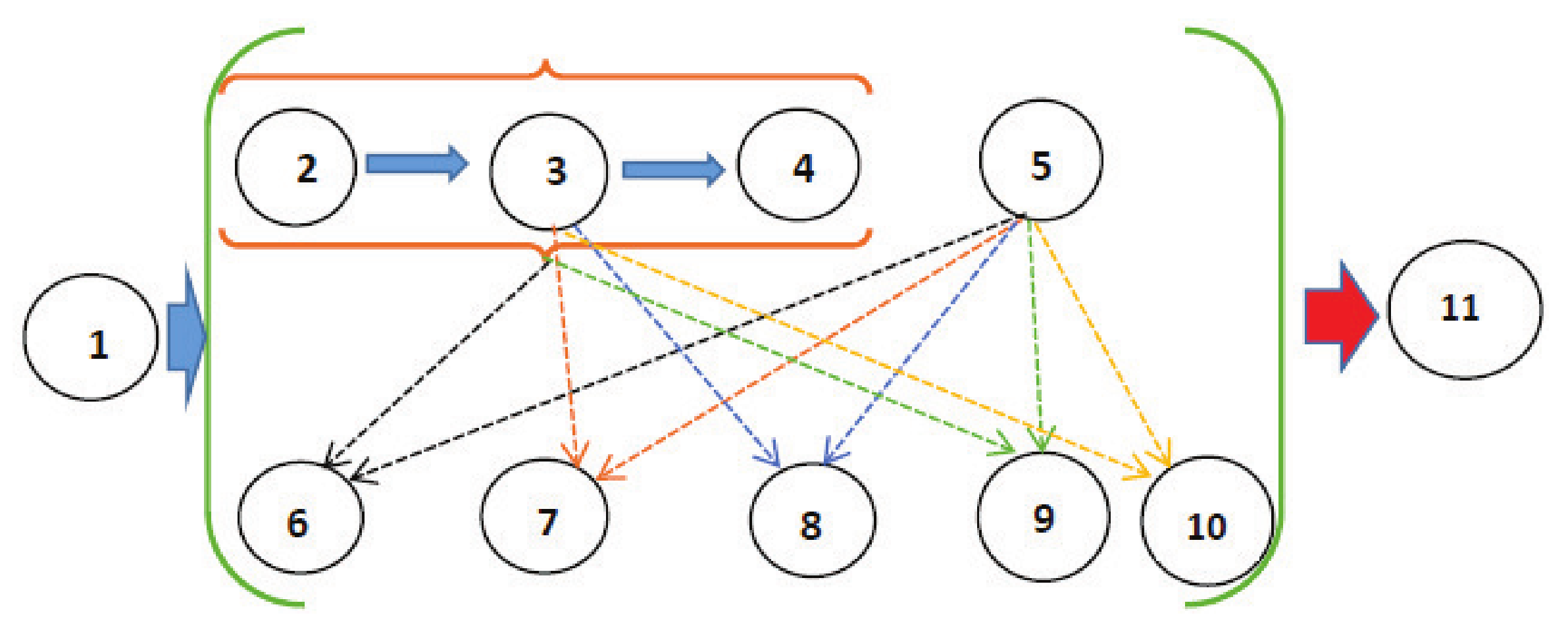
Figure 1. On the diagram, the dotted arrows indicate which sections are necessary to construct one or the other parameters of the QS and its environment.
Symmetry 13 01546 g001
Figure 2. The column (a) shows different phases ( t = 0.1 ps, t = 0.7 ps and t = 2 ps) of the evolution of the distribution of free classical fields P ¯ 1 practically without dissipation (vacuum conditions) and the formation of a small classical environment in it. The column (b) shows the same stages in the evolution of classical fields with allowance for elastic and inelastic processes in an environment that lead to the formation of a bulk SCE in it.
Symmetry 13 01546 g002
Figure 3. The column (a) shows snapshots of the probability distributions of the SQE in a quantum vacuum at the time t = 2 p s , for the quantum numbers n = 0 , n = 1 and n = 2 , respectively. Column (b) shows the probability distributions of SQE in TB, consisting of a dense medium at the same quantum numbers and time t = 2 p s . It is easy to see from these images that the distributions of the environmental fields differ greatly depending on the quantum number n.
Symmetry 13 01546 g003
Figure 4. The first column shows snapshots of the steady-state probability distributions of various quantum states of a 2D oscillator in a quantum vacuum. The second column shows the stationary probability distributions of a 2D oscillator when the environment is dense matter. We performed calculations up to the time t = 10 ps and made sure that all distributions reached their limits of statistical equilibrium.
Symmetry 13 01546 g004
Table 1. Initial data for numerical simulation the distribution of environmental fields.
α λ ν Ω 1 , 2 + Δ t ¯ Δ u ¯ 1 = Δ u ¯ 2 Gaussian  Distribution b 1
1.0 10 3 101.0954 10 5 0.025 a = b = 0.5 , σ = 500 6.94 × 10 4
1.0 10 3 −100.8944 10 5 0.025 a = b = 0.5 , σ = 500 1.56 × 10 3
Table 2. Initial data for numerical simulation the distribution of environmental fields.
α λ ν Ω 1 , 2 + Δ t ¯ Δ u ¯ 1 = Δ u ¯ 2 Gaussian  Distribution b 1
1.0  2.5 10   1.0954  2× 10 5 0.025 a = b = 0.5 , σ = 500 1.736
1.0  2.5 −10  0.8944  2× 10 5 0.025 a = b = 0.5 , σ = 500 3.906
Publisher’s Note: MDPI stays neutral with regard to jurisdictional claims in published maps and institutional affiliations.