Abstract
Because the two-dimensional coupled ecosystem has perfect symmetry, the dynamical behavior of symmetric dynamical system is discussed. The analysis of the dynamical behavior of a two-dimensional coupled ecosystem with stochastic parameters is explored in this paper. Firstly, a two-dimensional coupled ecosystem with stochastic parameters is established, it is transformed into a deterministic equivalent system by orthogonal polynomial approximation. Then, analysis of the dynamical behaviour of equivalently deterministic coupled ecosystems is performed using stability theory. At last, we analyzed the dynamical behaviour of non-trivial points by means of the mathematics analysis method and found the influence of random parameters on asymptotic stability in coupled ecosystem is prominent. The dynamical behaviour analysis results were verified by numerical simulation.
1. Introduction
Ecosystems provide the material goods and the natural environment on which humans depend, and ecosystem complexity has become a new hot spot in international ecological research. In recent years, due to the irrational exploitation and use of resources, human beings are facing the destruction of the balance of the natural ecosystem in which they live and the self-regulating role of maintaining this balance. Dynamics plays an important role in mathematics, aviation, economics, ecosystems, mechanics and finance [1,2,3,4,5,6]. Interaction relationships are the driving force behind ecosystem complexity, and in ecology, dynamical behaviour has a large impact on this system, with bifurcation and chaos occurring, causing system collapse, etc.
Discrete difference equation modeling of population ecology for the analytical study of the evolution of biological clock populations. The mathematical ecologist May has suggested in an influential 1976 paper published in Nature [7], a journal that demystifies the non-linear nature of ecology, that many ecosystems exhibit remarkable complexity in both structure and dynamics, which has been used to predict the response of ecosystems to human interference [8,9], and is the earliest example of a bifurcation from a multiplicative cycle leading to chaos. Nonlinear dynamical theory has been widely used in ecology, populations, epidemics, gene expression, neural networks and other fields [10]. The literature [11] examines the analysis of travel agency competition in a population ecology model and analyses the different results that emerge from competition between travel agencies under different parameters. Hastings [12], Udwadia [13] and Lloyd [14] et al. explored the chaotic dynamics of a two-dimensional logistic mapping of insect populations to populations in ecology.
The literature [15] investigates chaotic control with symbiotic effects of two groups of discrete coupled logistic models, The literature [16] couples two one-dimensional logistic models and studies their dynamical behaviour, and the text studies two-dimensional logistic models and derives universal characteristics of logistics leading from regular motion to chaos. The literature [17] discusses the stability and bifurcation of a class of two-dimensional discrete dynamical systems using positive regular type theory. The literature [18] applies the theory of local branching of dynamical systems to discuss the bifurcation analysis of a two-dimensional discrete system. The literature [19] studied and analyzed the two-dimensional logistic mapping bifurcation control. Xu Wei et al. studied the effects of noise and survival environment on predation systems [20] and the stochastic dynamics of the evolution of two competing populations [21]. Chaotic characterisation of two-dimensional stochastic coupled logistic mappings in the literature [22] reveals the law of the probability density function of the system orbit on the system state. Wantao Jia et al. studied Stochastic Dynamics of a Time-Delayed Ecosystem Driven by Poisson White Noise Excitation [23]; Literature [24] and [25] study dynamical systems with small random perturbations; D.G. Anderson studied the fundamental solution of a linear parabolic equation containing a small parameter [26]; A. Devinatz, R. Ellis and A. Friedman studied the asymptotic behavior of the first real eigenvalue of the second order elliptic operator with a small parameter in the higher derivatives [27]. Yi Wang et al. studied Analysis of Spatiotemporal Dynamic and Bifurcation in a Wetland Ecosystem [28]. Population interactions are often influenced by a number of environmental factors, and stochastic ecosystems have been paid a great deal of attention [29]. Some phenomena in nature, social sciences, economics and engineering are hiding many dynamic relationships that can be described by deterministic or stochastic systems. Since these random factors cannot be ignored, various random systems will be considered. And these stochastic factors determine the trends of complex systems in the real world. Therefore, it is quite necessary to research the dynamical in stochastic systems. At the same time, some scholars have researched the dynamic behavior and dynamic control problems of stochastic systems with random parameters, for example, bifurcation and chaos and so on [30,31,32,33,34,35].
However, the stability studies about a nonlinear stochastic coupling ecosystem with random parameters are few. In fact, the natural increase of many populations is always inevitably subjected to some stochastic disturbances, such as the external environment and intrinsic growth rate. It’s significant from the points of biological view to study the nature of the stochastic dynamics system, such as stability and bifurcation, etc. of dynamical behavior. Advances in ecosystem modeling have focused on the deepening of population dynamics models; ecosystems place more emphasis on the interactions between the parts of the system. The study of population dynamics is one of the central questions in classical ecological research and has been a major topic in the field of ecosystems. Thus, the dynamic behavior of two-dimensional stochastic coupling ecosystem is worth focusing on. In spite of the research results on the two-dimensional stochastic system already studied, there are a little studies on the influence of randomness on dynamic behavior. Furthermore, to our knowledge, the influence on the dynamic behavior of the two-dimensional stochastic coupling ecosystem with internal random parameters has not been found in the existing literature.
Motivated by the above discussions, we studied the two-dimensional stochastic coupling ecosystem. As far as we know, a stochastic two-dimensional system with random parameters, as a mathematical model, is closer to the real world under given statistical conditions. In the real ecosystem, considering the inherent randomness of population coupling coefficient, a two-dimensional stochastic coupling ecosystem model with stochastic coupling coefficient was established, which was described as a stochastic system. In this paper, the dynamic behavior of this kind of two-dimensional stochastic coupling ecosystem is studied by orthogonal polynomial approximation.
2. Materials and Methods
The logistic model in ecology was published by mathematical ecologist May in Nature in 1976 [7], and May was the first to study the results of research with multiplicative periodic bifurcation leading to chaos; its mapping equation is as follows:
According to Euler’s method, its differential form is obtained.
The two-dimensional coupled system can be obtained after iterative solution; the coupling system has perfect symmetry.
When , the two-dimensional coupled system of symmetry can be reduced to [22].
where , it is called the coupling coefficient.
Consider a two-dimensional ecosystem of symmetry with stochastic parameters
where is a stochastic parameter which can be expressed as
where is the deterministic parameter, and is regarded as strength of random disturbance, is the random variable defined on nonnegative set integer , which obeys density function , and is consists of independent equally distributed random variables, and . The equilibrium point of the system can be obtained by using the Brower fixed-point theorem and ; point is not of certain ecological significance, and is selected for system dynamics behavior analysis.
In this article we discuss the stability with the nontrivial equilibrium . We make the translation transformation, , .
Then Equation (5) is changed as follows:
According to the orthogonal polynomial approximation theory in Hilbert Space [35], the response of the system (7) can be indicated approximately by the following form
where represents the -th orthogonal polynomial, and M represents the largest order of the polynomials we retain.
Substituting Equations (6) and (8) into Equation (7), we obtain
With the aid of cycle recurrence formula of orthogonal polynomial
the stochastic term and the nonlinear term in the right equation of Equation (9) can be respectively expressed as follows,
where by the polynomial orthogonal approximation principle, are a power function coefficient of order of . Meanwhile, the stochastic term in the right equation of Equation (9) can be written as follows:
So, the two-dimensional ecosystem of symmetry with stochastic parameters is transformed as
where , , , , , , and are zero by the principle of approximation. We chose the stochastic variable with Poisson distribution with standard deviation . The weight orthogonal polynomial in Equation (10) is chosen as Charlier polynomial. The coefficients are respectively. Multiply both sides of system (17) by in sequence and take exception with respect to , where is after standardization of polynomial.
Based on orthogonal polynomial approximation of discrete stochastic function in the Hilbert spaces and the orthogonality of Charlier orthogonal polynomials, we can finally get the equivalently deterministic coupled ecosystems. We select and approximately obtain the equivalent deterministic system
Using mathematical software Maple, , , , can be calculated as follows:
Then the approximate stochastic response of the original two-dimensional coupled ecosystem with stochastic parameters can be expressed as
the sample response of mean parameter system (SMR) and the ensemble mean response of it (EMR) are indicated as
We take initial conditions of Equation (18) and the same initial condition of the deterministic system as follows, namely
3. Results
Analysis of the asymptotic stability in the stochastic parameter two-dimensional coupled ecosystem is based on Equation (7). The equivalent deterministic system Equation (18) can be expressed as
where is the coefficient matrix
For Equation (18), the Jacobian matrix at the equilibrium point is
and the characteristic equation as
where are the coefficients of Equation (28)
Lemma 1 ([36]).
Let the characteristic polynomial of the Equation (25) matrix be , when all roots of are in the unit circle under the following sufficient conditions
, , , , , , .
Where , , , , , , ,,
Lemma 2 ([36]).
For Equation (25),
- (1)
- The zero solution of system (18) is stable if all the characteristic roots of matrix A have a modulus no greater than 1 and the characteristic roots with modulus equal to 1 are unipartite.
- (2)
- If all the characteristic roots of matrix A have a modulus less than 1, the zero solution of system (18) is asymptotically stable.
- (3)
- If the matrix A has characteristic roots whose mode is greater than 1, the zero solution of the system (18) is unstable.
Theorem 1.
The functions are constructed by Jury criterion
Whenand, obtainTherefore the two-dimensional coupled ecosystem equilibrium point is the asymptotically stable point.
Proof.
Where
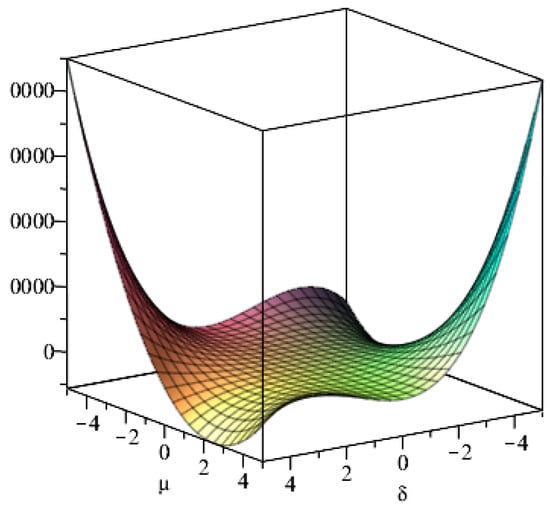
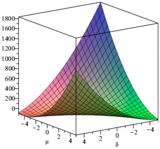
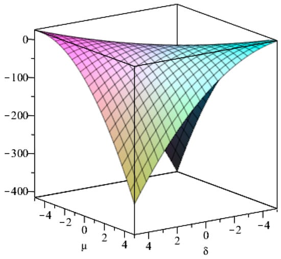
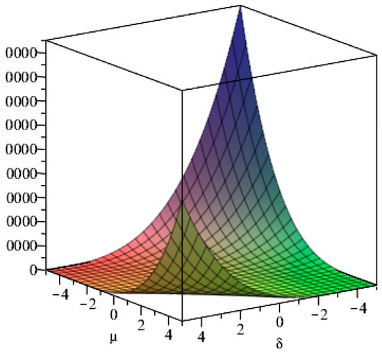
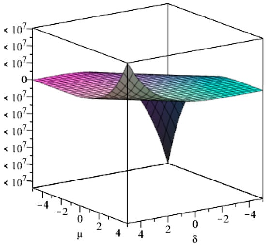
when then there are and , in order to show more clearly the relationship between and , , the image of with respect to , , is derived by mathematical software as follows.
It can be seen from Figure 1, Figure 2, Figure 3, Figure 4 and Figure 5 that when and are taken to be reasonably positive, it is clear that is satisfying Lemma 1, which further leads to the two-dimensional coupled ecosystem equilibrium point being the asymptotically stable point. □

Figure 1.
Image of the function with respect to , .

Figure 2.
Image of the function with respect to , .

Figure 3.
Image of the function with respect to , .

Figure 4.
Image of the function with respect to , .

Figure 5.
Image of the function with respect to , .
Theorem 2.
When and , the equilibrium point of two-dimensional coupled ecosystem is unstable; as and change, the system will bifurcate until chaos occurs.
Proof.
Equation (28) was solved using mathematical software and the theory related to characteristic equations, resulting in two characteristic roots that are not equal to 1 as , . If , then . If , then . Because , then , therefore . From Lemma 2 it follows that the equilibrium point is unstable. □
The above derivation was verified by numerical simulation, and some phenomena were obtained. When the strength of random , the two-dimensional stochastic ecosystem is investigated (5) can be turned into a deterministic original two-dimensional coupled system. Because Point is not of certain ecological significance, and is selected for system dynamics behavior analysis, the original system equilibrium point is . For ease of calculation and processing, it is sufficient to obtain the new system according to the coordinate translation transformation and consider the dynamic behaviour of the zero-equilibrium point. When the stochastic intensity is , the system is stable at the equilibrium point, which means that the ecological population system is stable.
When the coupling coefficient , the two populations are not coupled and do not affect each other, and each of the two populations in the ecosystem tends to be stable. Figure 6 shows that the two clusters do not affect each other with no restrictions on environmental capacity.
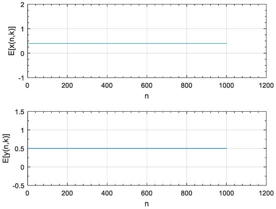
Figure 6.
Diagram of the history of the system when .
As the coupling stochastic intensity increases, the ecosystem dynamics change. Figure 7a–e is a graph of the time course of the increasing stochastic intensity of the system in the range , indicating that the equilibrium point of the two-dimensional stochastic coupled ecosystem is asymptotically stable, effectively validating the theoretical results of Theorem 1. It can be concluded from the figure that the system tends to asymptotically stabilise rapidly as the intensity continues to increase, reaching asymptotic stability in advance. Figure 8 shows the phase track diagram of a two-dimensional randomly coupled ecosystem. The asymptotic stability of the equilibrium point can also be clearly seen through the phase track diagram of the system in Figure 8; Figure 8b is a partial enlargement of Figure 8a.
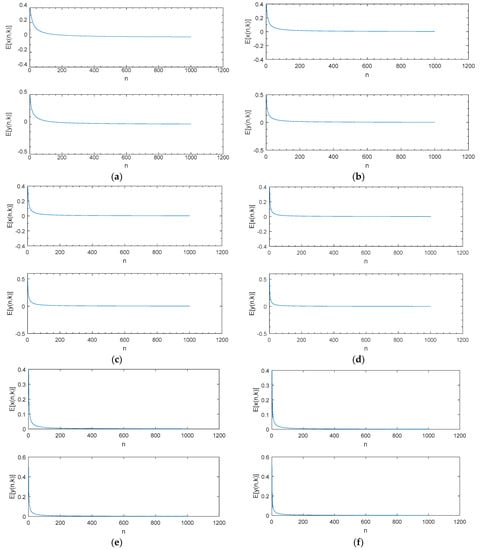
Figure 7.
Two-dimensional stochastic ecosystem time history diagram when . (and (a–f) are time course diagrams for two-dimensional random ecosystems with random intensities of 0.1, 0.2, 0.3, 0.4, 0.5, 0.6, respectively).
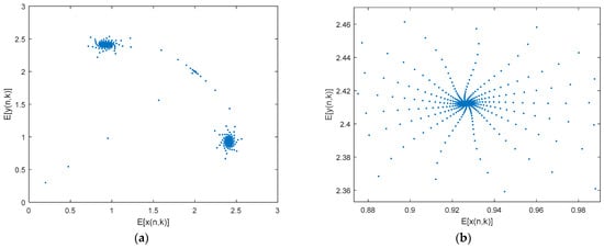
Figure 8.
(a) is an asymptotically stable phase track diagram for a two-dimensional stochastic ecosystem equilibrium point, (b) is a partial enlargement of (a).
When , according to the system history diagram shown in Figure 9, the system dynamics behaviour will change and its system equilibrium point is unstable; the random intensity also affects the system dynamics behaviour, effectively verifying the result of Theorem 2.
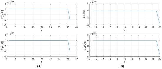
Figure 9.
Two-dimensional stochastic ecosystem time history diagram when . (and (a,b)are time course diagrams for two-dimensional random ecosystems with random intensities of 0.9, 1.2, respectively).
Figure 10 shows the system phase course diagram of a two-dimensional randomly coupled ecosystem with increasing random intensity. Analysis by numerical simulation methods shows that with increasing random intensity, the equilibrium points of the two-dimensional randomly coupled ecosystem becomes unstable, the dynamical behaviour changes continuously and the system shows bifurcation phenomenon, period phenomenon and frequency locking phenomenon. At the same time, it can be concluded from the bifurcation diagram of the system, Figure 11, that the random intensity will induce the bifurcation of the ecosystem until the emergence of complex dynamical behaviour such as chaotic phenomena; Figure 11b is a partial enlargement of Figure 11a.
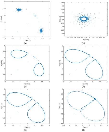
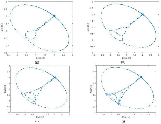
Figure 10.
Two-dimensional stochastic ecosystem phase track diagram when . ((a,c–j) are two-dimensional random ecosystem phase trajectories with random intensities of 0.7, 0.8, 0.9, 1.0, 1.2, 1.3, 1.4, 1.6, 1.7 respectively, and (b) is a partial enlargement of (a)).
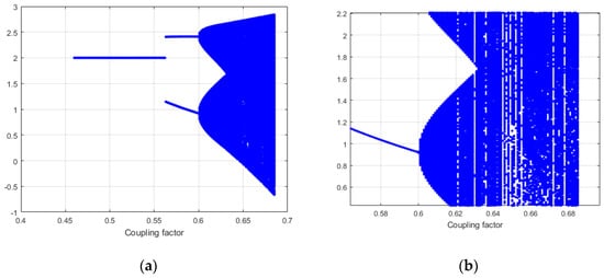
Figure 11.
(a) is two-dimensional stochastic ecosystem bifurcation diagram when , and (b) is a partial enlargement of (a).
Based on theoretical analysis and numerical simulations, we have found that in the two-dimensional randomly coupled ecosystem, we can know that within this parameter of the system, and , the equilibrium point of the system is asymptotically stable within this parameter of the system, , and , the equilibrium point of the system is unstable. Comparing to the deterministic system, the bifurcation and chaos with the variation of bifurcation parameter also occurs. Random intensity obviously affects the dynamical behaviour of its stochastic system, and stochastic intensity induces bifurcation until complex dynamics such as chaos emerge. The more stochastic influence, the more the stability of the population ecosystem is compromised, to the detriment of the stability of the ecosystem.
4. Conclusions
In this paper, the orthogonal polynomial approximation theory of discrete random function is applied to study the dynamical behaviour in a two-dimensional coupled ecosystem of symmetry with random parameters. By the mathematics analysis method, we have discovered that in the two-dimensional coupled ecosystem with stochastic parameters, as the random intensity or statistical parameters of random variables are increased, stability of nontrivial equilibrium in the stochastic system causes changes to occur. The influence of random parameters on asymptotic stability is prominent. Stochastic intensity induces bifurcation until complex dynamics such as chaos emerge. The more stochastic influence, the more the stability of the population ecosystem is compromised, to the detriment of the stability of the ecosystem. These results are different from the results in the deterministic system, which are characterized accurately by the stability of realistic models, revealing the dynamic mechanisms within ecosystems by numerical analysis.
Author Contributions
X.L. contributed significantly to analysis, manuscript preparation and wrote the manuscript. F.S. helped perform the analysis with constructive discussions. All authors have read and agreed to the published version of the manuscript.
Funding
This research received no external funding.
Institutional Review Board Statement
Not applicable.
Informed Consent Statement
Not applicable.
Data Availability Statement
No data were used to support this study.
Conflicts of Interest
The authors declare that they have no conflicts of interest.
References
- Li, D.M.; Ma, Z.F. Looking to the Future of Mathematical Ecology and Ecological Modelling. Acta Ecol. Sinica 2000, 20, 1083–1089. [Google Scholar]
- Liu, Q.K.; Zhang, Z.J.; Chen, X.M.; Li, Y.H. Stability Analysis of Enterprises Competition Based on Ecological Model. Math. Pract. Theory 2016, 46, 1–7. [Google Scholar]
- Chen, X.X.; Song, G.H.; Wang, X.J.; Li, Z.Y. Stability and Hopf Bifurcation of a Kind of Pinus Koraiensis Ecological System with Time Delay. J. Biomath. 2014, 29, 577–585. [Google Scholar]
- Jiang, H.B.; Li, X.Z.-P. Bifurcation Analysis of Complex Behavior in the Logistic Map via Periodic Impulsive Force. Acta Phys. Sin. 2013, 62, 120508. [Google Scholar]
- Zan, Q.T. Study on the Complicated Dynamlcal Behaviors of Nonlinear Ecosystem. Appl. Math. Mech. 1988, 9, 925–931. [Google Scholar]
- Niu, S.Y.; Jin, Y.F. Stability Analysis of a Stochastic Predator-Prey Model with Harrison Function Response. J. Dyn. Control 2016, 14, 276–282. [Google Scholar]
- May, R.M. Simple Mathematical Models with Very Complicated Dynamics. Nature 1976, 261, 459–467. [Google Scholar] [CrossRef]
- Scheffer, M.; Carpenter, S.; Foley, J.A.; Folke, C.; Walker, B. Catastrophic Shifts in Ecosystems. Nature 2001, 413, 591–596. [Google Scholar] [CrossRef]
- Kefi, S.; Rietkerk, M.; Alados, C.L.; Pueyo, Y.; Papanastasis, V.P.; ElAich, A.; De Ruiter, P.C. Spatial Vegetation Patterns and Imminent Desertification in Mediterranean Arid Ecosystems. Nature 2007, 449, 213–217. [Google Scholar] [CrossRef]
- Jia, X.Y.; Wu, Y. An Overview on Progess of Interdisciplinary Studies of Dynamics and Life Sciences. J. Dyn. Control. 2017, 15, 279–288. [Google Scholar]
- Zhang, L.Q.; Ding, B.Y. Competition Analysis of Travel Agencies Based on the Population Ecology Model. J. Henan Sci. Tech. 2014, 2, 278–286. [Google Scholar]
- Hastings, A. Complex Interactions Between Dispersal and Dynamics: Lessons from Coupled Logistic Equations. Ecology 1993, 74, 1362–1372. [Google Scholar] [CrossRef]
- Udwadia, F.E.; Raju, N. Dynamics of Coupled Nonlinear Maps and Its Application to Ecological Modeling. Appl. Math. Comput. 1997, 82, 137–179. [Google Scholar] [CrossRef]
- Alun, L.L. The Coupled Logistic Map: A Simple Model for the Effects of Spatial Heterogeneity on Population Dynamics. J. Theor. Biol. 1995, 173, 217–230. [Google Scholar]
- Fu, J.C.; Liu, C.L.; Jing, Y.W.; Zhang, S.Y. Chaos Control of Two Species Discrete Coupling Logistic Model with Symbiotic Interaction. J. Biomath. 2011, 26, 99–107. [Google Scholar]
- Ricardo, L.R. Complex Behavior in a Discrete Coupled Logistic Model for the Symbiotic Interaction of Two Species. Math. Biosci. Eng. 2004, 1, 307–324. [Google Scholar]
- Hou, A.Y.; Jiang, X.W. The Stability and Bifurcation of a Class of Two Dimensional Discrete Dynamical Systems. Math. Theory Appl. 2010, 28, 84–88. [Google Scholar]
- Huang, H.Q. The Bifurcation Analysis of one Discrete-Time system. J. Jiaying Univ. Nat. Sci. 2010, 28, 22–26. [Google Scholar]
- Zong, X.P.; Geng, J.; Wang, P. Bifurcation Control of the Coupled Logistic Mapping. Inf. Control 2011, 40, 343–351. [Google Scholar]
- Xu, W.; Qi, L.Y.; Gao, W.T. Effects of Noises and Habitat Complexity in the Prey-Predator Ecosystem. Appl. Math. Mech. 2013, 34, 162–171. [Google Scholar]
- Xie, W.X.; Cai, L.; Yue, X.L.; Lei, Y.M.; Xu, W. Information Entropies and Dynamics in the Stochastic Ecosystem of Two Competing Species. Acta Phys. Sin. 2012, 61, 170509. [Google Scholar]
- Yu, W.H.; Gao, S.L. Chaotic Characteristics of Two-Dimensional Random Coupled Logistic Map. J. Sichuan Univ. Nat. Sci. Ed. 2019, 56, 581–587. [Google Scholar]
- Jia, W.T.; Xu, Y.; Li, D.X. Stochastic Dynamics of a Time-Delayed Ecosystem Driven by Poisson White Noise Excitation. Entropy 2018, 20, 143. [Google Scholar] [CrossRef] [PubMed]
- Anderson, R.F.; Oray, S. Small Random Perturbations of Dynamical Systems with Reflecting Boundary. Nagoya Math. J. 1976, 60, 189–216. [Google Scholar] [CrossRef][Green Version]
- Freidman, A. Small Random Pertubations of Dynamical Systems and Applications to Parabolic Equations. Indiana Univ. Math. J. 1974, 24, 533–553. [Google Scholar] [CrossRef][Green Version]
- Anderson, D.G. The Fundamental Solution of a Linear Parabolic, Equation Containing a Small Parameter. Ill. J. Math. 1959, 3, 580–619. [Google Scholar]
- Devinatz, A.; Ellis, R.; Friedman, A. The Asymptotic Behavior of the First Real Eigenvalue of the Second Order Elliptic Operator with a Small Parameter in the Higher Derivatives. Indiana Univ. Math. J. 1973, 74, 991–1011. [Google Scholar]
- Wang, Y.; Zhao, M.; Yu, H.; Dai, C.; Mei, D.; Wang, Q.; Ma, Z. Analysis of Spatiotemporal Dynamic and Bifurcation in a Wetland Ecosystem. Discret. Dyn. Nat. Soc. 2015, 2015. [Google Scholar] [CrossRef]
- Miśkiewicz, J.; Ausloos, M. A Logistic Map Approach to Economic Cycles. Phys. A Stat. Mech. Its Appl. 2004, 336, 206–214. [Google Scholar] [CrossRef][Green Version]
- Feng, T.; Meng, X.Z. Stochastic Dynamics of a Predator-prey System with Disease in Predator. J. Shandong Univ. Sci. Technol. 2017, 36, 99–110. [Google Scholar]
- Ma, S.J.; Dong, D. The Asymptotic Stability Analysis in Stochastic Logistic Model with Poisson Growth Coefficient. Theor. Appl. Mech. Lett. 2014, 4, 0130041–0130049. [Google Scholar] [CrossRef][Green Version]
- Liu, Y.; Liu, Q.; Liu, Z. Dynamical Behaviors of a Stochastic Delay Logistic System with Impulsive Toxicant Input in a Polluted Environment. J. Theor. Biol. 2013, 329, 1–5. [Google Scholar] [CrossRef]
- Ma, S.J.; Dong, D.; Zheng, J. Generalized Synchronization of Stochastic Discrete Chaotic System with Poisson Distribution Coefficient. Discret. Dyn. Nat. Soc. 2013, 2013. [Google Scholar] [CrossRef]
- Xu, W. Numerical Analysis Methods for Stochastic Dynamics System; Science Press: Beijing, China, 2013. [Google Scholar]
- Donsker, M.D.; Varadhan, S.R.S. Asymptotic for the Wiener Saussage. Comm. Pure Appl. Math. 1975, 28, 525–565. [Google Scholar] [CrossRef]
- Elaydi, S. An. Introduction to Difference Equations, 3rd ed.; Springer: Berlin/Heidelberg, Germany, 2005. [Google Scholar]
Publisher’s Note: MDPI stays neutral with regard to jurisdictional claims in published maps and institutional affiliations. |
© 2021 by the authors. Licensee MDPI, Basel, Switzerland. This article is an open access article distributed under the terms and conditions of the Creative Commons Attribution (CC BY) license (https://creativecommons.org/licenses/by/4.0/).