Abstract
Predictive models may be considered a tool to ensure food quality as they provide insights that support decision making on the design of processes, such as fermentation. Objective: To formulate a mathematical model that describes the growth of lactic acid bacteria (LAB) in batch fermentation. Methodology: Based on real-life experimental data from eight LAB strains, we formulated a primary model in the form of a third-degree polynomial function that successfully describes the four phases observed in LAB growth, i.e., lag, exponential, stationary, and death. Our cubic mathematical model allows us to understand the fundamental nonlinear dynamics of LAB as well as its time-variant dependencies. Parameters of the model are written in terms of initial biomass, maximum biomass, maximum growth rate, and lag phase duration. Further, a statistical analysis was performed to compare our cubic primary model with the ones proposed by Gompertz, Baranyi, and Vázquez-Murado by computing the coefficient of determination , the residual sum of squares , and the Akaike Information Criterion . Results: The average statistical results from the cubic model are as follows: providing a better fit than the other three models, and , where both values are lower than the other models considered in this study. Conclusion: The cubic primary model formulated in this work describes the behavior of biomass as it accurately represents the four phases of biomass growth in batch fermentation process.
1. Introduction
Lactic Acid Bacteria (LAB) refer to a group of microorganisms that share certain morphological, physiological, and metabolic characteristics. They have the peculiarity of producing lactic acid from several carbohydrates through a process known as microbial fermentation. They are normally found in cultures such as milk, whey, and pickles [1,2]. The Danish microbiologist Orla-Jensen said that “True lactic acid bacteria are a large group of cocci and Gram positive, immobile, spore free bacilli, which produce lactic acid in the fermentation of sugar” [3]. Currently, LAB have a primary role in the food industry, as they are used to acidify and preserve food. Further, they contribute to texture, taste, smell, and scent development in all kinds of fermented foods [4,5].
In the industry, most fermentation is carried out through batch culture. This means that only a culture medium with the necessary nutrients is added to the fermenter, and this is incubated for the growth of bacteria and the production of its primary metabolite. During the time of incubation, nothing other than oxygen is added [6]. Hence, the bacterial growth follows an asymmetric cell division (ACD), which is a conserved mechanism evolved to generate cellular diversity. A key principle of ACD is the establishment of distinct sibling cell fates by mechanisms linked to mitosis [7]. ACD also occurs in the development and physiology of unicellular organisms ranging from bacterial species to yeasts and flagellates [8,9]. In these organisms, ACD underlies replicative aging as a means of maintaining the immortality of the mitotically proliferating population [10].
LAB are very demanding microorganisms and need a set of growing factors, including sugars such as carbohydrates, as well as amino acids and vitamins. Therefore, LAB can only grow in a medium that supplies these nutrients [3]. The interest in the physiology of LAB has been studied by its industrial importance and potential use of genetic engineering in strain optimization. For example, in the particular case of Lactococcus lactis spp. lactis, a minimal growth medium should contain glucose, acetate, vitamins, and amino acids [11]. Milk is the medium that contains all these nutrients. For this reason, LAB are used as starter cultures for the preparation and preservation of dairy products, such as acidified milk, yogurt, butter, cream, and cheese [1]. In batch fermentation, bacteria cannot grow exponentially indefinitely. The latter due to bacteria depleting nutrients as it grows, changes in the chemical composition of the medium , and toxic compounds that are accumulated. The characteristic curve of bacterial growth is composed by four phases: (i) lag, (ii) exponential, (iii) stationary, and (iv) death. Lactic acid production occurs during the reproduction of LAB; the accumulation of this and other organic acids decrease the of the medium, which made culture conditions become more selective; hence, the more acid-tolerant bacterium will prevail.
The total number of cells in fermentation are usually represented by a logarithmic scale, and normally, at the end of this process, one can see values from up to CFU/mL (Cell-Forming Units per milliliter) [2]. In addition to nutritional requirements, temperature is one of the most important factors in LAB growth. Furthermore, there is an optimal temperature and other environmental conditions for which these microorganisms present a higher growth rate [4]. LAB are acid-tolerant and may grow either at values as low as or as high as . Usually, most of LAB strains grow at values between 4 and [1].
In microbiology, several mathematical models have been developed to predict the behavior of microorganisms on the influence of different factors in culture. This branch is known as predictive microbiology, and it aims to study the response of bacteria to environmental factors that can be controlled, such as temperature, , and water volume, among others. In this sense, a tool may be formulated to ensure both quality and safety of products to estimate their useful lifetime and to make decisions regarding the composition and design of fermented products [12]. Mathematical models that relate biomass production and time are called primary models, while those that describe the relationship between primary models parameters and environmental conditions are known as secondary models [13]. Some of these models are discussed below.
The Gompertz equation, formulated in 1825, is one of the most used in predictive microbiology. It is based on an exponential relationship between the growth rate and the density of a population. This equation was formulated to describe the law of human mortality. However, years later, it was adapted and re-parametrized for its use in microbiology [14]. Giraud et al. [15] observed that variations resulted in a decrease in the growth rate when measuring the fermentation performance of L. plantarum at a controlled between and . Baranyi et al. [16] applied a non-autonomous differential equation to describe the dynamics of growing bacterial cultures. Based on more than 500 growth curves, the statistical properties of this equation were compared to the Gompertz approach, which is the most commonly used in food microbiology. After these results, Baranyi and Roberts [17] proposed a growth model where a single variable represents the physiological state of cells. The lag phase period is determined by the value of this variable at inoculation and by the post-inoculation environment. The model was able to describe bacterial growth in an environment where factors, such as temperature and , change over time. Nicolai et al. [18] constructed a dynamical model for the growth of LAB in vacuum-packed meat. The model was divided into two parts: one part describing the fermentation and the other describing the evolution in the liquid surface layer. These models were given as two differential equations and two algebraic equations, respectively. Passos et al. [19] developed an unstructured model to describe bacterial growth, substrate utilization, and lactic acid production by L. plantarum in cucumber juice. They also developed an equation that relates the specific mortality rate and the sodium chloride concentration. Drosinos et al. [20] formulated an empirical model to describe the growth and production of bacteriocin by Leuconostoc mesenteroides under different conditions of and temperature. Further, a De Man, Rogosa, and Sharpe (MRS) broth was used as a growth medium in the fermenter. Vázquez and Murado [21] proposed a model based on the re-parametrized logistic equation to describe fermentation kinetics of lactic acid production by Lactococcus lactis and Pediococcus acidilactici in a batch system. Da Silva et al. [22] studied the growth of L. plantarum, W. viridescens, and L. sakei under different isothermal culture conditions at temperatures of 4, 8, 12, 16, 20, and 30 ∘C. They determined that LAB growth was strongly influenced by the culture temperature and created new models that allowed them to predict growth at temperatures ranging from 4 to 30 ∘C. Dalcanton et al. [23] built a response model of the growth rate of L. plantarum as a function of temperature, , and concentrations of and sodium lactate .
Despite the existence of several mathematical models in the literature that describe the behavior of LAB during the fermentation process in its three phases, i.e., lag, exponential, and stationary phases, they do not include the death phase in these models. In batch fermentation, after the stationary state, the depletion of nutrients in the culture medium occurs, and therefore, the death phase begins and should be considered in these models. By not taking the death phase into account, a problem arises when trying to fit real-life experimental data with the models usually used in predictive microbiology. Therefore, the objective of this research is to formulate a time-variant mathematical model that describes the growth of LAB, including its death phase in batch fermentation.
The remainder of this paper proceeds as follows. In Section 2, we present the real-life experimental data concerning biomass growth for eight LAB strains; we formulate our cubic mathematical and explain each parameter; and the most important kinetic models identified in the literature are explored. In Section 3, a statistical analysis is performed to establish which model better fits the experimental data, and these results are illustrated by means of several numerical simulations. Finally, discussions are described in Section 4, and conclusions are given in Section 5.
2. Materials and Methods
2.1. Experimental Data
Eight LAB strains were investigated in the present study; all of them isolated from autochthonous fermented milk. This process was performed based on certain desirable characteristics and against microbial spoilage [24]. LAB strains were incubated for 48 h at a temperature of 37 ∘C in reconstituted milk powder to produce acidification. Biomass production was measured every 6 h by means of the Neubauer cell counting chamber. Two repetitions were performed for each strain, and the average was calculated as the final concentration value at each corresponding hour. The total biomass concentration was written on a logarithmic scale with units given in (CFU/mL). Furthermore, the experimental data were conditioned by a moving mean filter to minimize noisy measurements in the biomass concentration and to better illustrate LAB growth in each of its four phases, which we mentioned before as lag, exponential, stationary, and death. The results are illustrated in Figure 1, and the overall dynamics allow us to formulate a third-degree polynomial that will be discussed in the following section.
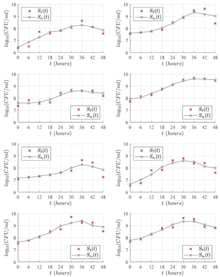
Figure 1.
Time-evolution for the eight LAB strains, each × mark represents the average value of the two measurements made with Neubauer cell counting chamber on each strain. The ∘ mark represents the results obtained when applying a moving mean filter to smooth the experimental data.
2.2. Mathematical Modelling: Cubic Polynomial Model
In order to formulate a mathematical model to describe the time-evolution for the eight different strains of LAB in the 48 h of the process (see Figure 1), we proposed the following third-degree polynomial
where describes biomass growth dynamics in (CFU/mL) as a function of time, is the initial biomass in each experiment, and coefficients represent the relationships between maximum biomass, lag phase time, and maximum growth rate. Differential calculus concepts were applied to write coefficients as functions of the desired set of parameters. Now, let us compute the first derivative, as it represents growth rate as follows
to find the maximum increase in biomass, which is denoted as , we calculate the local extremums as indicated below
from the latter, it is evident that at , there is a minimum. Therefore, the time when the maximum biomass increase occurs is given at
Then, by the substitution of Equation (3) into Equation (1), one can calculate as follows
Now, by computing the second derivative of Equation (1), which is given below
and the time to the inflection point is computed as follows from Equation (5)
then, this value is evaluated in Equation (2) to calculate the maximum growth rate, which is denoted as . This parameter represents the slope of the tangent at the inflection point, and its value is given by the next result
The total amount of biomass at the inflection point, which is given as h, is obtained by evaluating Equation (6) into Equation (1), and the corresponding result is given below
therefore, the inflection point is located at the following coordinate
Now, in order to find the lag time-period , the intersection of the tangent line on the inflection point at the t-axis was calculated, as illustrated in Figure 2.
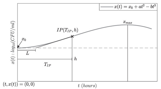
Figure 2.
A graphic representation to compute the lag time-period parameter L.
Hence, by applying the point-slope equation, we formulate the following
and by isolating L from Equation (9), the following result is obtained
then, replace and h with Equations (6) and (8), respectively. Thus, L is rewritten as follows
Equations (4) and (10) relate parameters of interest with coefficients a and b of Equation (1). Therefore, one can isolate a from Equation (10) as follows
and substitute it into Equation (4) to find the value of b as indicated below
then, Equation (12) should be replaced by Equation (11) to determine the final value of coefficient a; hence
2.3. Primary Models
Numerical simulations were made to illustrate and analyze the time-evolution of our model and the other three chosen from the literature. These models are presented below. First, let us introduce the Gompertz model [14]:
Then, the Baranyi model [17], which is given as follows:
where and may be written as indicated below [25]:
Now, the model from Vázquez-Murado [21]:
In each model, represents the initial biomass, the maximum biomass, the maximum growth rate, and L the lag phase time. Further, these three models were selected because they are among the most cited in predictive microbiology, and their parameters are the same as in our cubic primary model (14). Parameter values were calculated from the smoothed data of the eight LAB strains (see in Figure 1). Parameters and are, respectively, the initial and the maximum biomass values. The value of the parameter is computed as shown below
where and are taken from the smoothed experimental data, i.e., a given value and its previous one. The latter is divided by the time interval of the measurements, which, in this particular case, 6 h, and since we have nine measurements, then . Furthermore, it should be noted that Equation (10) was used to calculate the Lag time period, L. The results concerning all necessary parameter values are shown in Table 1.

Table 1.
The results concerning all parameter values for the four mathematical models under study respecting each LAB strain illustrated in Figure 1.
3. Results
In order to validate our model, a statistical analysis was performed to calculate and compare the descriptive capacity of the cubic model (14) and models (15)–(17). The statistic used was the coefficient of determination , which measures the goodness of fit of a non-linear model according to experimental data. Its calculation is made based on the sum of squared residuals , and the explanatory capacity of a model is better the closer is to 1, see Section 11-8.2 [26].
Figure 3, Figure 4, Figure 5 and Figure 6 illustrate the dynamics of the cubic model and its comparison with analyzed models from the literature concerning the experimental data of eight LAB strains, . One can see in Figure 3 that the cubic model describes the four expected growth phases in batch fermentation, while the Gompertz model, see Figure 4; the Baranyi model, see Figure 5; and Vázquez-Murado model, see Figure 6; only describe up to the stationary phase, which caused the value to be higher for these models, and therefore, the results concerning and indicate a poorer fit. The lag phase time was around 5 to 9 h. The maximum biomass growth was reached between 30 and 36 h for each of the strains, and from that time, the death phase begins.
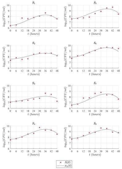
Figure 3.
Predictions of the cubic model compared with the experimental data .
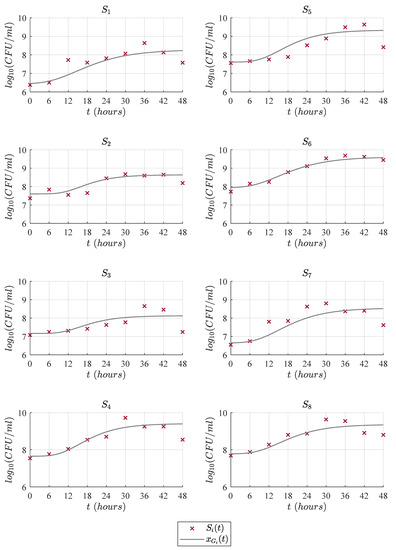
Figure 4.
Predictions of Gompertz model compared with the experimental data .
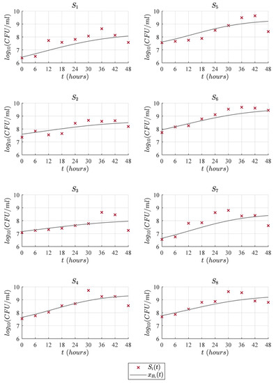
Figure 5.
Predictions of the Baranyi model compared with the experimental data .
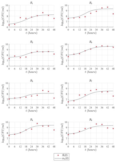
Figure 6.
Predictions of the Vázquez-Murado compared with the experimental data .
According to our numerical simulations, one can observe that the proposed cubic model (14) and the other primary models (15)–(17) have a good adjustment in the lag phase, as is shown by each solution and the corresponding experimental data. Concerning the exponential phase, the Baranyi model is slightly above the others. However, this model has a lower growth rate, which causes a delay when reaching the maximum concentration, approximately at 48 h, while other models reach this value at around 30 or 36 h. Regarding the maximum biomass growth, the three primary models remain in the stationary phase, while the experimental data goes to the death phase. Therefore, the of these models is higher than the cubic model, as this one better fits the observed data in this last phase. Table 2 shows the results of and for the cubic, Gompertz, Baranyi, and Vázquez-Murado models with respect to the experimental data illustrated in Figure 1.
Table 2.
The results of and for each mathematical model.
Now, concerning strain 1, the cubic model presented an of and, consequently, a higher value of given by compared to Gompertz, Baranyi and Vázquez-Murado models, which obtained an equal to , , and and an equal to , , and , respectively. For strain 2, the highest value was for the cubic model with , followed closely by the Vázquez-Murado and Gompertz models with and , respectively, while the Baranyi model had a result of . In the particular case of strain 3, all models had a lower adjustment when comparing them with the other seven strains. However, the best fit was for the cubic model with an of , while the Gompertz model obtained a value of , Baranyi obtained , and Vázquez-Murado . For strain 4, very similar values were obtained for Gompertz, and Vázquez-Murado models, and , respectively, while the cubic model obtained a result of , and Baranyi got a value of . In strain 5, the cubic model had an value of , which was higher than the Gompertz , Baranyi , and Vazquez-Murado . Strain 6 had a better fit for all models. The Vázquez-Murado model had an of , Gompertz , cubic model , and the lowest value was for Baranyi, with . These higher values are due to fact that the experimental data for this strain have fewer outliers, as seen in Figure 1, and its death phase is lower compared to the other strains. Strain 7 had a better fit for the cubic model, with an of , than the Gompertz , Baranyi , and Vázquez-Murado models. Finally, as in most cases, the cubic model had the best fit for strain 8 with an value of , while Gompertz and Vázquez-Murado obtained, respectively, and . In general, the cubic model had higher values of than the rest of the models, except in strain 6, where the Vázquez-Murado model had the better fit to the experimental data. The latter was due to the data not yet presenting the death phase as the other strains in the 48 h of the experiment.
Furthermore, the Akaike Information Criterion test was performed, which allows us to determine which model better fits the observed data. To calculate this value, the goodness of fit between predictions of models and experimental data is considered through the while penalizing models that have a greater number of parameters due to these becoming more complex for its practice [27]. Table 3 shows results for every mathematical model.
Table 3.
results for each mathematical model.
By taking the latter into account, the model that better fits the experimental data is the one with the lowest value. For strain 1, the lowest AIC was for the cubic model with a value of , while Gompertz, Baranyi, and Vázquez-Murado models obtained values of , , and , respectively. In strain 2, the cubic model had the lowest , with a value of , and the Gompertz model and the Vázquez-Murado model had similar results, and respectively, while the Baranyi had a value of . The cubic model fitted better to the experimental data of strain 3 with an of , followed by Gompertz with , Vázquez-Murado with , and finally, Baranyi with . Again, for strain 4, according to the values, the cubic model () was better than the Gompertz (), Baranyi (), and Vázquez-Murado () models. In strain 5, the best value was for the cubic model (), while Gompertz obtained , Baranyi , and Vázquez-Murado . In strain 6, very close values were obtained for Vazquez-Murado and Gompertz , but the Vázquez-Murado model was slightly better. The cubic model had a value of . On the other hand, Baranyi model had a lower fit with an of . For strain 7, the lowest value was obtained for the cubic model , while Gompertz had a value of , Baranyi , and Vázquez-Murado . Finally, regarding strain 8, the cubic model had the better fit to the experimental data based on its value (), and Baranyi had the worst fit (), while Gompertz and Vázquez-Murado obtained results of and , respectively.
After analyzing the statistical results, it is evident that our formulated cubic primary model better fits the experimental data because it was the one that presented the lowest in general and therefore had higher values for the in all LAB strains but number 6, which had a higher value with the Vázquez-Murado model . However, the result for the cubic model was of , which is still a good value concerning this parameter. Therefore, based on the results for the , , and the , we can establish that the cubic primary model (14) better represents the overall dynamics of the experimental data for the eight LAB strains under study in this research.
4. Discussion
In predictive microbiology, primary models based on sigmoidal functions are usually used. Among the most common models, we have the Gompertz [14], the Baranyi [17], and the Vázquez-Murado [21] models. Nonetheless, the latter only describe the first three growth phases, i.e., lag phase, exponential growth, and the stationary state. According to Buchanan et al. [28] and Garre et al. [29], these phases are sufficient to fit experimental data for growth models. However, according to Mandigan et al. [6], in batch fermentation, the bacterial population presents a death phase due to nutrient depletion in the culture medium. Therefore, when adjusting these models to observed data in this kind of fermentation, values of greater discrepancy are found in the death phase between the experimental data and approximated values. Chatterjee et al. [30] incorporated the death phase into the Gompertz model to better describe the behavior of E. coli and S. aureus. Studies by Bevilacqua et al. [31] were focused on demonstrating the importance of the death phase of microorganisms and its impact on the shelf life of food. Solano et al. [32] evaluated the capacity of five models, including the Gompertz, Baranyi, and Vázquez-Murado, to predict acid production in lactic fermentation of fishing products, and they found that models with the lowest residual variance were those of Gompertz and Baranyi. Further, this study shows that the Vázquez-Murado model failed to give an adequate adjustment for lactic fermentation. In the same way, Zwietering et al. [33] managed to describe the behavior of L. plantarum in an MRS medium with the Gompertz model, while the Vázquez-Murado logistic model was not suitable to accurately approximate the experimental data. In contrast, Kedia et al. [34] obtained a good fit with the Vázquez-Murado model for L. reuteri, L. plantarum, and L. acidophilus in oat fractions. Da Silva et al. [22] studied the growth of L. plantarum, W. viridescens, and L. sakei in vacuum-packed meats, and, as well as Baty and Delignette [35] who studied different growth models for various LAB, all authors in these two works found that the Baranyi model has a slightly better fit than the Gompertz model.
According to the and values, it can be established that the cubic model has a better fit to the experimental data with average values of and . There was not enough difference between the average values for the Gompertz model with and , while the Vázquez-Murado had average results of and . Regarding the Baranyi model, the average results were as follows and . Further, the overall adjustment to the experimental data for the four primary models under study is illustrated in Figure 3, Figure 4, Figure 5 and Figure 6.
In this research, the four primary models presented a good adjustment in the lag phase and reached the maximum growth registered in the experimental data. However, the maximum growth rate value had a greater impact on the adjustment of the exponential growth phase, in which the cubic model was the one that had the better fit. Nonetheless, in order to get a good fit with primary models, it is necessary to measure the largest amount of experimental data with the greatest possible continuity, which will ensure a better prediction by the models. In the batch fermentation process performed for this work, the eight LAB strains showed outliers, which could be due to the method applied for the measurements. Therefore, the experimental data had to be smoothed to calculate all required parameters for each mathematical model. It is important to consider that outliers are present in all real-life data measurements, such as biomass growth.
In the cubic model, the parameter also influences the death phase of the biomass. The latter because a higher growth rate implies that the maximum biomass concentration will be reached, and due to the inherit dynamics of this kind of function, after reaching this maximum point, the biomass begins to decline. It is important to consider that if this mathematical model is simulated at time values further than 70 h, biomass will take negative values, which is not biologically feasible in real-life scenarios. However, this can be neglected because the fermentation process to produce acidified milk generally takes around 48 h, and it is not necessary to predict the behavior of this variable beyond this time, as this is the final desired product. Predictive models aim to ensure food quality and provide a tool that supports decision-making on fermentation design. Therefore, based on the results and as it is illustrated in Figure 3, Figure 4, Figure 5 and Figure 6, a decision can be made to perform a fermentation process under the same culture conditions only up to 36 h, i.e., when the maximum biomass growth is reached for this type of fermented milk.
5. Conclusions
A time-variant mathematical model given in the form of a third-order polynomial was formulated to describe the growth dynamics over a period of 48 h for eight LAB strains. Our so-called cubic primary model (Equation (14)) was constructed with the parameters that are frequently used in other primary models, i.e, biomass initial concentration, ; lag phase time, ; maximum growth rate, ; and maximum growth, . Furthermore, both the numerical simulations and the statistical results concerning , , and the support our statement that the cubic model accurately represents the four biomass growth phases in the batch fermentation process when comparing it with three other models that are among the most cited in predictive microbiology literature.
Author Contributions
Conceptualization, Y.S., O.M.R.-Q. and R.R.-H.; methodology, Y.S. and E.R.; software, P.A.V.; validation, Y.S., B.E.G. and P.A.V.; formal analysis, Y.S. and P.A.V.; investigation, E.R. and A.C.F.-G.; resources, B.E.G.; data curation, B.E.G.; writing—original draft preparation, Y.S. and E.R.; writing—review and editing, P.A.V.; visualization, Y.S. and P.A.V.; supervision, Y.S. and P.A.V.; project administration, Y.S. All authors have read and agreed to the published version of the manuscript.
Funding
Authors of this work were supported by different projects indicated as follows: Yolocuauhtli Salazar by the TecNM project 10083.21-P: Modelizado de la dinámica de crecimiento de microorganismos durante la fermentación de leche fresca with number; Paul A. Valle by the TecNM project 9951.21-P Modelizado computacional y experimentos in silico aplicados al análisis y control de sistemas biológicos; Blanca E. Garcia and O. Miriam Rutiaga-Quiñones by the TecNM project 5973.19-P Desarrollo de un potencial inoculante para la producción de Jocoque.
Institutional Review Board Statement
Not applicable.
Informed Consent Statement
Not applicable.
Data Availability Statement
Data are contained within the article.
Acknowledgments
Emmanuel Rodriguez and Blanca E. Garcia express their recognition to the National Council of Science and Technology of Mexico (Consejo Nacional de Ciencia y Tecnología, CONACyT) for the financial support during their postgraduate studies under their scholarship agreement.
Conflicts of Interest
The authors declare no conflict of interest.
Abbreviations
The following abbreviations and symbols are used in this manuscript:
| LAB | Lactic Acid Bacteria |
| ACD | Asymmetric Cell Division |
| MRS | De Man, Rogosa and Sharpe |
| Coefficient of determination | |
| RSS | Residual Sum of Squares |
| AIC | Akaike Information Criterion |
References
- Axelsson, L. Lactic Acid Bacteria: Classification and Physiology. In Lactic Acid Bacteria: Microbiology and Functional Aspects, 2nd ed.; Marcel Dekker, Inc.: New York, NY, USA, 1998; pp. 1–72. [Google Scholar]
- Sheeladevi, A.; Ramanathan, N. Lactic acid production using lactic acid bacteria under optimized conditions. Int. J. Pharm. Biol. Arch. 2011, 2, 1686–1691. [Google Scholar]
- Axelsson, L.; Ahrné, S. Lactic acid bacteria. In Applied Microbial Systematics; Springer: Berlin/Heidelberg, Germany, 2000; pp. 367–388. [Google Scholar] [CrossRef]
- Carr, F.J.; Chill, D.; Maida, N. The Lactic Acid Bacteria: A Literature Survey. Crit. Rev. Microbiol. 2002, 28, 281–370. [Google Scholar] [CrossRef]
- Novik, G.; Meerovskaya, O.; Savich, V. Waste degradation and utilization by lactic acid bacteria: Use of lactic acid bacteria in production of food additives, bioenergy and biogas. In Food Additive; InTech: London, UK, 2017; p. 105. [Google Scholar] [CrossRef]
- Mandigan, M.; Martinko, J.; Bender, K.; Buckley, D.; Stahl, D. Brock Biology of Microorganisms, 14th ed.; Pearson: Boston, MA, USA, 2015. [Google Scholar]
- Sunchu, B.; Cabernard, C. Principles and mechanisms of asymmetric cell division. Development 2020, 147, dev167650. [Google Scholar] [CrossRef]
- Bi, E.; Park, H.O. Cell polarization and cytokinesis in budding yeast. Genetics 2012, 191, 347–387. [Google Scholar] [CrossRef]
- Rotureau, B.; Subota, I.; Buisson, J.; Bastin, P. A new asymmetric division contributes to the continuous production of infective trypanosomes in the tsetse fly. Development 2012, 139, 1842–1850. [Google Scholar] [CrossRef] [PubMed]
- Li, R. The art of choreographing asymmetric cell division. Dev. Cell 2013, 25, 439–450. [Google Scholar] [CrossRef] [PubMed]
- Jensen, P.R.; Hammer, K. Minimal requirements for exponential growth of Lactococcus lactis. Appl. Environ. Microbiol. 1993, 59, 4363–4366. [Google Scholar] [CrossRef] [PubMed]
- Guillier, L. Predictive microbiology models and operational readiness. Procedia Food Sci. 2016, 7, 133–136. [Google Scholar] [CrossRef][Green Version]
- Stavropoulou, E.; Bezirtzoglou, E. Predictive Modeling of Microbial Behavior in Food. Foods 2019, 8, 654. [Google Scholar] [CrossRef] [PubMed]
- Gompertz, B. XXIV. On the nature of the function expressive of the law of human mortality, and on a new mode of determining the value of life contingencies. In A letter to Francis Baily, Esq. FRS & c; Philosophical Transactions of the Royal Society of London: London, UK, 1825; Volume 1, pp. 513–583. [Google Scholar] [CrossRef]
- Giraud, E.; Lelong, B.; Raimbault, M. Influence of pH and initial lactate concentration on the growth of Lactobacillus plantarum. Appl. Microbiol. Biotechnol. 1991, 36, 96–99. [Google Scholar] [CrossRef]
- Baranyi, J.; Roberts, T.; McClure, P. A non-autonomous differential equation to model bacterial growth. Food Microbiol. 1993, 10, 43–59. [Google Scholar] [CrossRef]
- Baranyi, J.; Roberts, T.A. A dynamic approach to predicting bacterial growth in food. Int. J. Food Microbiol. 1994, 23, 277–294. [Google Scholar] [CrossRef]
- Nicolai, B.; Van Impe, J.; Verlinden, B.; Martens, T.; Vandewalle, J.; De Baerdemaeker, J. Predictive modelling of surface growth of lactic acid bacteria in vacuum-packed meat. Food Microbiol. 1993, 10, 229–238. [Google Scholar] [CrossRef]
- Passos, F.V.; Fleming, H.P.; Ollis, D.F.; Felder, R.M.; McFeeters, R. Kinetics and modeling of lactic acid production by Lactobacillus plantarum. Appl. Environ. Microbiol. 1994, 60, 2627–2636. [Google Scholar] [CrossRef] [PubMed]
- Drosinos, E.; Mataragas, M.; Metaxopoulos, J. Modeling of growth and bacteriocin production by Leuconostoc mesenteroides E131. Meat Sci. 2006, 74, 690–696. [Google Scholar] [CrossRef] [PubMed]
- Vázquez, J.A.; Murado, M.A. Unstructured mathematical model for biomass, lactic acid and bacteriocin production by lactic acid bacteria in batch fermentation. J. Chem. Technol. Biotechnol. 2008, 83, 91–96. [Google Scholar] [CrossRef]
- Silva, A.P.R.d.; Longhi, D.A.; Dalcanton, F.; Aragão, G.M.F.d. Modelling the growth of lactic acid bacteria at different temperatures. Braz. Arch. Biol. Technol. 2018, 61. [Google Scholar] [CrossRef]
- Dalcanton, F.; Carrasco, E.; Pérez-Rodríguez, F.; Posada-Izquierdo, G.D.; Falcão de Aragão, G.M.; García-Gimeno, R.M. Modeling the combined effects of temperature, pH, and sodium chloride and sodium lactate concentrations on the growth rate of Lactobacillus plantarum ATCC 8014. J. Food Qual. 2018, 2018, 1726761. [Google Scholar] [CrossRef]
- Leroy, F.; De Vuyst, L. Lactic acid bacteria as functional starter cultures for the food fermentation industry. Trends Food Sci. Technol. 2004, 15, 67–78. [Google Scholar] [CrossRef]
- Powell, C.D.; López, S.; France, J. New Insights into Modelling Bacterial Growth with Reference to the Fish Pathogen Flavobacterium psychrophilum. Animals 2020, 10, 435. [Google Scholar] [CrossRef] [PubMed]
- Montgomery, D.C.; Runger, G.C. Applied Statistics and Probability for Engineers, 6th ed.; John Wiley and Sons: Hoboken, NJ, USA, 2013; p. 920. [Google Scholar]
- Burnham, K.P.; Anderson, D.R. Multimodel inference: Understanding AIC and BIC in model selection. Sociol. Methods Res. 2004, 33, 261–304. [Google Scholar] [CrossRef]
- Buchanan, R.L.; Whiting, R.C.; Damert, W.C. When is simple good enough: A comparison of the Gompertz, Baranyi, and three-phase linear models for fitting bacterial growth curves. Food Microbiol. 1997, 14, 313–326. [Google Scholar] [CrossRef]
- Garre Pérez, A.; Egea Larrosa, J.; Fernández Escámez, P. Modelos matemáticos para la descripción del crecimiento de microorganismos patógenos en alimentos. Anuario de Jóvenes Investigadores 2016, 9, 160–163. [Google Scholar]
- Chatterjee, T.; Chatterjee, B.K.; Majumdar, D.; Chakrabarti, P. Antibacterial effect of silver nanoparticles and the modeling of bacterial growth kinetics using a modified Gompertz model. Biochim. Biophys. Acta Gen. Subj. 2015, 1850, 299–306. [Google Scholar] [CrossRef]
- Bevilacqua, A.; Speranza, B.; Sinigaglia, M.; Corbo, M.R. A Focus on the Death Kinetics in Predictive Microbiology: Benefits and Limits of the Most Important Models and Some Tools Dealing with Their Application in Foods. Foods 2015, 4, 565–580. [Google Scholar] [CrossRef]
- Solano-Cornejo, M.A.; Vidaurre-Ruiz, J.M. Application of unstructured kinetic models in the lactic fermentation modeling of the fishery by-products. Sci. Agropecu. 2017, 8, 367–375. [Google Scholar] [CrossRef][Green Version]
- Zwietering, M.; Jongenburger, I.; Rombouts, F.; Van’t Riet, K. Modeling of the bacterial growth curve. Appl. Environ. Microbiol. 1990, 56, 1875–1881. [Google Scholar] [CrossRef] [PubMed]
- Kedia, G.; Vázquez, J.A.; Pandiella, S.S. Evaluation of the fermentability of oat fractions obtained by debranning using lactic acid bacteria. J. Appl. Microbiol. 2008, 105, 1227–1237. [Google Scholar] [CrossRef][Green Version]
- Baty, F.; Delignette-Muller, M.L. Estimating the bacterial lag time: Which model, which precision? Int. J. Food Microbiol. 2004, 91, 261–277. [Google Scholar] [CrossRef] [PubMed]


Publisher’s Note: MDPI stays neutral with regard to jurisdictional claims in published maps and institutional affiliations. |
© 2021 by the authors. Licensee MDPI, Basel, Switzerland. This article is an open access article distributed under the terms and conditions of the Creative Commons Attribution (CC BY) license (https://creativecommons.org/licenses/by/4.0/).