On Systems of Active Particles Perturbed by Symmetric Bounded Noises: A Multiscale Kinetic Approach

Abstract

We consider an ensemble of active particles, i.e., of agents endowed by internal variables u(t). Namely, we assume that the nonlinear dynamics of u is perturbed by realistic bounded symmetric stochastic perturbations acting nonlinearly or linearly. In the absence of birth, death and interactions of the agents (BDIA) the system evolution is ruled by a multidimensional Hypo-Elliptical Fokker–Plank Equation (HEFPE). In presence of nonlocal BDIA, the resulting family of models is thus a Partial Integro-differential Equation with hypo-elliptical terms. In the numerical simulations we focus on a simple case where the unperturbed dynamics of the agents is of logistic type and the bounded perturbations are of the Doering–Cai–Lin noise or the Arctan bounded noise. We then find the evolution and the steady state of the HEFPE. The steady state density is, in some cases, multimodal due to noise-induced transitions. Then we assume the steady state density as the initial condition for the full system evolution. Namely we modeled the vital dynamics of the agents as logistic nonlocal, as it depends on the whole size of the population. Our simulations suggest that both the steady states density and the total population size strongly depends on the type of bounded noise. Phenomena as transitions to bimodality and to asymmetry also occur.

1. Introduction

Two of the more active fields of application of statistical physics to biology are theoretical population dynamics, mathematical epidemiology (including behavioral aspects [1,2]), sociophysics [3,4,5] and mathematical oncology [6,7]. In these fields, the importance of multiscale phenomena has been recognized in the last twenty years. Many important approaches are based on individual based models [8,9,10]. Another very important approach is based on classical and recent development of nonlinear statistical physics: the theory of active particles [11,12,13,14,15,16,17,18,19,20]. This is a multiscale mean field theory that allows us to link the dynamics of internal variables, named activity, to the macroscale of the interactions between large sets of agents [12,13,14,15,16,17]. Bellomo and coworkers stressed in particular two concepts are of the utmost relevance in applying theory of active particles to living matter: (i) new agents that are generated can have an activity different than the one of their parent agent; (ii) non destructive interactions between two agents of the same or of different species (e.g., tumor cells and immune system effectors) can induce a change of activity level in both agents. Among the most recent developments of the Bellomo theories we cite: (i) the theory of thermostatted active particles, which allows to impose physically backgrounded constraints to the activity of individuals, developed by Bianca and Menale [21,22,23]; (ii) the stochastic evolutionary theory of tumor adaptation developed by Clairambault, Delitala, Lorenzi and coworkers [24,25,26,27,28,29]. Finally, it is worth mentioning the mathematical modeling of Darwinian species emergence by Volpert and colleagues that represent the evolution of active particles uniquely subject to a Brownian force and logistic non-local growth [30,31,32].

In the framework of Bellomo’s theories, Firmani, Preziosi and Guerri (FPG) [33] (see also [34]) first modeled in a detailed way how to pass from the deterministic dynamics of the activity variable of single individual agent to the dynamics of the densities of interacting populations. In the FPG model the dynamics of the agent’s activity was assumed to be deterministic. This led the authors to define a generalization of the Liouville’s equation to model the temporal evolution of the densities (w.r.t. the agents’ activities) of the interacting populations.

However important this approach may be, it constitutes an approximation of the real world behavior. Indeed, on the one hand it has been stressed that fundamental biological phenomena arise from the microscale presence of internal additive noise, i.e., infinitesimal spontaneous stochastic fluctuations of the activity [24,25,26,27,28,29]. In the case where the activity represents phenotypic defining variables, this represents the spontaneous phenotypic changes [24,25,26,27,28,29]. On the other hand, individual agent activities are perturbed by many unknown internal and external interaction, which can only be statistically known.

Modeling such stochastic extrinsic perturbations is less straightforward than one could think. Namely, one could be tempted to extend a deterministic model by including multiplicative Gaussian white or colored perturbations. Although allowing nice analytical or semi-analytical inferences, this approach can lead to artifacts, most often hidden. A major example is the following [35,36] modeling in the above-mentioned way the perturbations affecting an anti-tumor cytotoxic therapy implies that for a substantial part of time therapy adds tumor cells instead of killing them. A second ‘hidden’ but equally important artifact is also induced: an excessive instantaneous killing of tumor cells. Finally, Gaussian White noise perturbations cannot be applied to parameters on which a system depends nonlinearly, and often even Gaussian colored perturbation cannot.

These and other critical issues imply that bounded stochastic processes ought to be used in most case in biophysics: an increasingly important approach [36]. In last twenty years about, a large body of scientific work has been devoted to the application of bounded stochastic processes in statistical physics and to biophysics. Some key application can be listed: noise-induced transitions [37], stochastic and parametric resonance [38], bifurcation theory [39], fractional and nonlinear mechanics [40,41,42], mathematical oncology [43,44], cell biology [45], ecology and environment [46,47] and neurosciences [48].

As a consequence, the above mentioned interplays can be modeled by assuming that the dynamics is affected by bounded stochastic perturbations. This is our key assumption here, which will lead us to define a family of partial integro-differential models that extends hypo-elliptic nonlinear Fokker–Planck equation. Similar but not identical since, duty to the presence of nontrivial non–local birth and death terms, in our case the integral of the population density is the time-varying population size, and not the unity, as in the nonlinear FP equation. The above-mentioned hypoellipticity is a key point since it is implied from the assumption that the perturbations are symmetric bounded stochastic processes.

This work is organized in three parts. In the first part, we summarize and slightly extend the FPG model in Section 2 and we extend it to take into the account stochastic white noise perturbations acting on the dynamic of all agents in Section 3. The second part of the work starts in Section 4, where we stress pitfalls that can occur by an acritical use of Gaussian white or colored noises. In the following Section 5 we derive the main family of models of this work, which models the dynamics of ensembles of active particles perturbed by realistic stochastic processes of bounded nature, and in Section 6 we briefly stress the possible occurrence, in specific models, of phase transitions. Finally, in Section 7 we formulate a specific model (belonging to the general family of models defined in Section 5) where the dynamics of the population of agents are given by a nonlocal generalized logistic model. The third part of this work is devoted to numerical simulations. First (Section 8) we summarize two ‘recipes’ to define and simulate three types of bounded stochastic processes. Then in Section 9 we briefly model the perturbations at level of each single agent as a logistic dynamics and in Section 10 we parameterize the various adopted functions. In Section 11, we numerically infer the steady state probability distribution of the FPE that described the collective dynamics of particles in absence of generation, death and interplay: this allows us to stress some interesting noise induced transitions phenomena. The steady state solution of the FPE is used in the following Section 12 as initial value of the full logistic non–local dynamics.

At the best of our knowledge, this work has some novelties of potential interest in statistical physics: it is the first kinetic model where the impact of bounded stochastic processes is included (resulting in hypo-ellictic integro-differential equations) and it is investigated its interplay with logistic non-local birth–death dynamics. Moreover, noise induced transition to bimodality and asymmetry are also observed.

2. A Slight Generalization of the FPG Model

In this section, we briefly summarize and slightly extend the FPG model [33,34] in case of a single population, and we frame it in the classical statistical mechanics. To start, let us suppose that the activity of an idealized agent is of the type

$$u^{\prime }=f\left(u\right),$$

(1)

where the state variable is called activity of the agent. In the general case u is vectorial but here for the sake of the notation simplicity we will suppose it scalar. Just to give some examples of activities we can mention: the level of proteins defining the degree of immunogenicity and ‘abnormality’ of a tumor cell [49], the level of activation for an immune system effector [49], the ‘level of effectiveness in performing the job that a species is expected to do’ in a multi species environment [50], the pair (opinion, connectivity) in models of opinion formation in social networks [51], the viral load for a subject during an epidemics [20]. Of course, a very important class of activities is the couple position–velocity $(x,v)$ [52].

We denote by

$$\rho (t,u)$$

the density of agents w.r.t. the time and to the activity variable u.

Let us now preliminary consider the very idealized case where the agents do not interplay and do not reproduce and die. In such a case, the dynamics of the ensemble of agent is nothing else than the dynamics of the distribution of an ensemble of particles in their phase space [53]. Thus, given the initial distribution of agents w.r.t. the activity u

$$\rho (0,u)={\rho }_0\left(u\right),$$

the evolution for $t>0$ of the ensemble of agents is given by the Liouville’s Equation [53]:

$${\partial }_t\rho +{\partial }_u\left(f\left(u\right)\rho \right)=0.$$

(2)

The physical interpretation of the term $f\left(u\right)\rho$ is straightforward: since $f\left(u\right)$ is the velocity in the activity state space, then $J=f\left(u\right)\rho$ is the current of active particles in that space, and Equation (2) is nothing else than the conservation law:

$${\partial }_t\rho +Div\left(J\right)=0.$$

Note that at variance to [33,34], where the FPG model is derived by a conservation law approach, here we focused on a probabilistic approach in view of the stochastic extension of next sections. Indeed, the Liouville equation is a particular case of the Fokker–Planck Equation [53].

The inclusion of the proliferation, death and inter-agents interaction gives the full model

$${\partial }_t\rho +{\partial }_u\left(f\left(u\right)\rho \right)=\mathcal{H}(\rho (.);N(.)),$$

(3)

where $\mathcal{H}\left(\rho \right(.);N(.\left)\right)$ is an integro-differential nonlinear operator that models: (i) agents’ birth, interaction and death; (ii) how the generation and interaction of agents modify their activity. For example, if the mother agent before asexual reproduction has an activity level $\widehat{u}$ then its m daughter agents, let us call them $D_1$, $D_2$, …, $D_m$, may have different activity levels ${\widehat{u}}_{D_1}\ne \widehat{u}$, …, ${\widehat{u}}_{D_m}\ne \widehat{u}$. We will later specify some noteworthy cases.

An important difference between the FPG model and the family of models (3) is that, at variance with the FPG model, the generation and destruction of agents here can be independent of agents interaction, as in the above example of asexual reproduction of agents.

Finally, we mention that the total size of the cellular population is given by the following integral:

$$N\left(t\right)={\int }_{D_u}\rho (t,u)du.$$

(4)

As far as the domain of the activity we will consider (as in [33]) a finite interval, for example

$$D_u=[0,u_M].$$

3. Impact of the Stochastic Fluctuations of the Activity

In this section, we introduce the study of the impact at the population scale of the stochastic perturbations acting on the dynamics of the activity u of each single agents. This is an important matter since in many complex systems composed by ensemble of individuals there can be the onset of emergent phenomena [54,55,56,57,58].

Due to unavoidable interactions with the external world and with the myriad of other internal processes (e.g., for cells: intra-cellular biomolecular networks) a far more realistic model of the evolution of the activity of the single agent is apparently

$$u^{\prime }=f\left(u\right)+g\left(u\right)\xi \left(t\right),$$

(5)

where $\xi \left(t\right)$ is a white noise and the stochastic differential equation is in the Ito interpretation (but one could consider the Stratonovich interpretation). A more realistic model will be considered in the next section.

In the absence of generation, death and of inter–agents interplay yields the dynamics of $\rho (t,u)$ is given by the following linear Fokker–Planck equation:

$${\partial }_t\rho +{\partial }_u\left(f\left(u\right)\rho \right)={\partial }_{uu}\left(\frac{g^2\left(u\right)}{2}\rho \right).$$

(6)

Note that at variance with the classical Fokker–Planck equation here it is

$${\int }_{D_u}\rho (t,u)du\ne 1$$

since it holds that

$$N\left(t\right)={\int }_{D_u}\rho (t,u)du=N_0,$$

where $N_0=N\left(0\right)$ is the initial size of the population (unchanged due to a assumption of no modification of the number of agents). Indeed, the total size of the population remains constant because of the lack of birth and of death events.

In presence of birth and death events and of inter–agents interactions, the Fokker–Planck-like Equation (2) becomes as follows:

$${\partial }_t\rho +{\partial }_u\left(f\left(u\right)\rho \right)={\partial }_{uu}\left(\frac{g^2\left(u\right)}{2}\rho \right)+\mathcal{H}(\rho (.);N(.)),$$

(7)

where $\mathcal{H}$ is an operator acting on the (present and past) agents’ distribution $\rho (.)$ and that can depend on the (present and past) population size $N\left(t\right)$.

Note that specific models where it holds that

$$g\left(u\right)=Constant,$$

i.e., the activity u has spontaneous stochastic fluctuations; have been investigated by Clairambault, Delitala, and Lorenzi and coworkers in a series of works (e.g., [24,25,26,27,28,29]) where the activity u represent phenotype variables and thus the additive noise represent spontaneous infinitesimal changes of phenotype.

4. Realistic Bounded Stochastic Perturbations of Agent’s Activity

Let us more closely analyze from the biological viewpoint the microscopic model (5). Namely, consider a model of the activity linearly depending on a positive parameter q:

$$u^{\prime }=a\left(u\right)+qb\left(u\right).$$

The stochastic fluctuations of the parameter q could be modeled as a white noise perturbations

$$u^{\prime }=a\left(u\right)+(q+q\xi \left(t\right))b\left(u\right),$$

(8)

where $\xi \left(t\right)$ is a white noise, characterized by $\mathcal{E}\left[\xi \right(t\left)\right]$ and $\mathcal{E}\left[\xi \right(t\left)\xi \right(t+\tau \left)\right]=\delta \left(\tau \right)$.

Thus, according to our previous the notation, corresponds to $f\left(u\right)=a\left(u\right)+qb\left(u\right)$ and $g\left(u\right)=qb\left(u\right)$. The fact is that writing in the Ito form [59]

$$du=a\left(u\right)dt+(qdt+qdB)b\left(u\right),$$

(9)

where $B\left(t\right)$ is a Brownian stochastic process [59], it immediately follow that in the realization

$$Prob(qdt+qdB<0)>0$$

(note that since $dB$ scales as $d{t}^{0.5}$ it follow that the occurrence of the event $qdt+qdB<0$ is quite frequent). In other words, the unbounded nature of the Gauss distribution renders negative the perturbed parameter q. Moreover, there is a second more subtle problem: the unbounded Gauss perturbation can also make the perturbed parameter q excessively large.

Both these two problems persists also if one uses a colored Gaussian perturbation instead of a Gauss white noise, or other non Gaussian unbounded perturbations.

A third and equally important problem is that if one has a general model nonlinearly depending on a parameter q

$$u^{\prime }=c(u;q),$$

then one cannot use white noise perturbations, and often one cannot use colored unbounded perturbations.

The solution is to use bounded stochastic perturbations [36]: $z\left(t\right)$ such that

$$z\left(t\right)q+q>0$$

and

$$z\left(t\right)q+q\le Q_{max}<\infty .$$

In turn $z\left(t\right)$ can depend on a (bounded or unbounded) noise y (which we will call support noise) by means of the following link function:

$$z\left(t\right)=\zeta \left(y\right(t\left)\right).$$

If y is unbounded, then $\zeta \left(y\right)$ is a bounded function, otherwise if y is itself bounded we assume $\zeta \left(y\right)=y$.

The problem of modeling the activity of a single agents becomes slightly more complex than in the case of white noise perturbations since at level of the individual agent one has two stochastic equations: the equation of the activity perturbed by the bounded noise y:

$$u^{\prime }=f(u,y),$$

(10)

where no white noise appears, and a model for the noise

$$y^{\prime }=k\left(y\right)+n\left(y\right)\eta \left(t\right),$$

(11)

which is independent of u, and where $\eta \left(t\right)$ is a white noise.

5. Macro-Scale Implication of the Boundedness of the Perturbations

The use of more realistic white noise perturbations implies that the resulting population-level model for the evolution of the density is quite more complex than in the case of Gaussian perturbations.

Indeed, in absence of generation, death and interplay we obtain a bidimensional Fokker–Planck equation because of the two stochastic state variables—$(u,y)$—which reads as follows:

$${\partial }_t\rho +{\partial }_u\left(f(u,y)\rho \right)+{\partial }_y\left(k\left(y\right)\rho \right)={\partial }_{yy}\left(\frac{n^2\left(y\right)}{2}\rho \right).$$

(12)

Note that the above equation is a degenerate diffusion-transport PDE since the u variable does not appear in the diffusion equation. The reason is that the microscopic equation for u does not contain a white noise term.

Finally, taking into the account the vital dynamics of the agents and their interactions yields the following model:

$${\partial }_t\rho +{\partial }_u\left(f(u,y)\rho \right)+{\partial }_y\left(k\left(y\right)\rho \right)={\partial }_{yy}\left(\frac{n^2\left(y\right)}{2}\rho \right)+\mathcal{H}(\rho (.);N(.)).$$

(13)

Remark 1.

Although the full density $\rho (t,u,y)$ is of interest, what in the practice really matters is the density ${\rho }^{eff}(t,u)$ unconditional to y, which is given by the following integral:

$${\rho }^{eff}(t,u)={\int }_{-B}^B\rho (t,u,y)dy.$$

(14)

6. Possibility of First and Second-Order Phase Transitions

The presence of $N\left(t\right)$ in the above-defined models has deep implications. Indeed, let us consider the search for steady state concentrations ${\varrho }_{ss}\left(u\right)$ (uniquely for the sake of the notation simplicity here we consider Gaussian perturbations):

$${\partial }_u\left(f\left(u\right){\varrho }_{ss}\left(u\right)\right)={\partial }_{uu}\left(\frac{g^2\left(u\right)}{2}{\varrho }_{ss}\left(u\right)\right)+\mathcal{H}({\varrho }_{ss}(.);N_{ss}).$$

(15)

Let us treat $N_{ss}$ as it were a parameter, and suppose now that we can find an analytical solution that will be denoted as follows:

$${\varrho }_{ss}(u,N_{ss};p),$$

where p denotes other parameters of the system.

This solution will have to verify the following self-consistency equation

$$N_{ss}={\int }_{D_u}{\varrho }_{ss}(u,N_{ss},p)du.$$

(16)

The above equation could have one or more solution, depending also on the values of the parameters p. The case of multiple solutions means that there are multiple steady state solutions. Thus, the dynamics of the system depend on the initial conditions and that by varying the parameter p first and second order phase transitions can be observed, with the switch from a scenario where the system has two (or more) stochastic attractors to a scenario with a unique stochastic attractors, which is the genuine landmark of phase transitions, as stressed by Shiino [60]. This is not surprising since the exact self-consistency Equation (16) is similar to the self-consistency equation of the approximated mean field Curie–Weiss theory [61,62].

7. A Generalized Logistic Growth of Agents

Up to now, we kept unspecified the functional $\mathcal{H}$, because we wanted to define a general family of models. In view of the simulations, here we consider the death and birth of agents in presence of competition for nutrients and space. As it happens in the reality we assume that the competition is not direct, i.e., two agents do not start a deadly battle for the last glass of water, but indirect. As such, in our specific example there are no interaction terms. This leads to decompose the operator $\mathcal{H}$ in two components, namely a birth component and a death component:

$$\mathcal{H}(\rho (.);N(.))={\mathcal{B}}_0(\rho (.);N\left(t\right))-{\mathcal{D}}_0(\rho (.);N\left(t\right)),$$

(17)

where we will call ${\mathcal{B}}_0$ the generation operator, and ${\mathcal{D}}_0$ the death operator

$${\partial }_t\rho +{\partial }_u\left(f\left(u\right)\rho \right)={\partial }_{uu}\left(\frac{g^2\left(u\right)}{2}\rho \right)+{\mathcal{B}}_0(\rho (.);N\left(t\right))-{\mathcal{D}}_0(\rho (.);N\left(t\right));$$

(18)

or in case of bounded perturbations:

$${\partial }_t\rho +{\partial }_u\left(f(u,y)\rho \right)+{\partial }_y\left(k\left(y\right)\rho \right)={\partial }_{yy}\left(\frac{n^2\left(y\right)}{2}\rho \right)+{\mathcal{B}}_0(\rho (.);N\left(t\right))-{\mathcal{D}}_0(\rho (.);N\left(t\right)).$$

(19)

As far as the death operator is concerned, a reasonable assumption is to set:

$${\mathcal{D}}_0(\rho (.);N\left(t\right))=\mu (u,N\left(t\right))\rho (t,u,y),$$

(20)

i.e., agents with activity u dies with a death rate $\mu$ that may depend on u and that, due to competition effects, depend on $N\left(t\right)$. since the dependence on $N\left(t\right)$ is due to competition effects, it yields that

$${\partial }_N\mu (u,N)>0.$$

For the sake of the simplicity, henceforward, we will only consider the following simple form for the death rate:

$$\mu (u,N\left(t\right))={\mu }_0\left(u\right)+{\mu }_1\left(u\right)N^a\left(t\right),$$

(21)

where $a>0$.

The operator ${\mathcal{B}}_0$ is less straightforward. First we suppose that agents around a value w of the activity have a reproduction rate $\alpha (w,N(t\left)\right)>0$ that depends on the activity w and that, due to the competition with other agents (causing lack of nutrients and of space), the rate is a decreasing function of the population size:

$${\partial }_N\alpha (w,N)<0.$$

The generated agents will have an activity u with a given probability density $\vartheta (u,w)$. More specifically, we will assume that $\vartheta (u,w)$ will has either mode or mean at w.

As far as the transition probability $\vartheta (u,w)$ is concerned, in case of a finite range of activities, $D_u=[0,u_M]$, one can employ a beta distribution

$$\vartheta (u,w)=\frac{1}{u_{M}B(p,q)}{\left(\frac{u}{u_M}\right)}^{p-1}{\left(1-\frac{u}{u_M}\right)}^{q-1}.$$

(22)

As far as the relationship between the value of the activities of mother and daughter agents, a natural choice could be the following:

(i) The average of the activity u of a daughter agent is equal to the activity w of the mother agent, which implies:

$$p=\left(\frac{w}{u_M-w}\right)q;$$

(23)

(ii) The mode of the activity u of a daughter agent is equal to the activity w of the mother agent, which implies:

$$p-1=\left(\frac{w}{u_M-w}\right)(q-1).$$

(24)

Finally, a particular but important case is the case where the daughter agents have the same activity of the mother agent:

$$\vartheta (u,w)={\delta }_{Dirac}(u-w).$$

Based on the above premises, we define:

$${\mathcal{B}}_0(\rho (.);N\left(t\right))={\int }_{D_u}\vartheta (u,w)\alpha (w,N\left(t\right))\rho (t,w,y)dw.$$

(25)

Formula (25) is particularly suited to the represent cell proliferation, which is characterized by an unequal division of metabolic constituents to daughter cells [63,64,65,66]. As far as the specific form of $\alpha (w,N(t\left)\right)$ are concerned, one can consider

$$\alpha (w,N)={\left({\alpha }_0\left(w\right)-{\alpha }_1\left(w\right)N^b\left(t\right)\right)}_{+},$$

(26)

or

$$\alpha (w,N)=\frac{{\alpha }_0\left(w\right)}{1+{\alpha }_1\left(w\right)N^b\left(t\right)}.$$

(27)

8. ‘Recipes’ to Model Bounded Noises

In this section, we shortly summarize two of the main methodologies used in the literature to generate bounded stochastic processes [36,67].

The first and most easy recipe to model a bounded stochastic perturbation consists of applying a bounded function, say $\beta \left(y\right)$, to an colored unbounded noise, for example the Orenstein–Uhlenbeck noise. This means

$$k\left(y\right)=-\frac{1}{\tau }y;$$

$$n\left(y\right)=\frac{\sqrt{2}\sigma }{\sqrt{\tau }};$$

$$f(u,y)=h(u,\zeta (y\left)\right).$$

(28)

Namely here we use the arctan noise, introduced in [67,68], in which:

$$\zeta \left(y\right)=B\frac{2}{\pi }Arctan\left(\frac{y}{Q}\right).$$

(29)

The rationale underlying the arctan noise defined by (29) is very simple: (i) the $Arctan$ function is bounded by the values $M=\pm \pi /2$; (ii) thus $(2/\pi )Arctan$ is bounded by $\pm 1$ and, as a consequence, $(2/\pi )Arctan$ is bounded by $\pm B$; (iii) the parameter Q ‘tunes’ the bounded noise: if $Q<<\sigma$ then (roughly speaking) $\zeta \left(y\right(t\left)\right)$ assumes mostly the two values $\pm B$, whereas if $Q>>\sigma$ then $\zeta \left(y\right(t\left)\right)$ is mostly proportional to y: $\zeta \left(y\right(t\left)\right)\approx 2By/\left(\pi Q\right)$.

Another and very general family of bounded stochastic processes, introduced in [69], can be obtained by assuming that

$$k\left(y\right)=-\frac{1}{\tau }y,$$

and imposing the condition

$$n(\pm 1)=0.$$

(30)

Condition (30) implies that

$$y^{\prime }{{|}_{y=1}<0\mathrm{AND}{y}^{\prime }|}_{y=-1}>0,$$

which in turn yields that if $y\left(0\right)\in [-1,1]$ then it $y\left(t\right)$ is bounded

$$y\left(t\right)\in [-1,1].$$

In this case the link function $\zeta \left(y\right)$ is simply $\zeta \left(y\right)=By$ An instance of this class of noises is the Doering–Cai–Lin noise, introduced in [69,70] and whose properties where studied in [71] where

$$n\left(y\right)=\sqrt{\frac{1}{(1+\delta )\tau }\left(1-y^2\right)},$$

(31)

where

$$\delta >-1,$$

whose stationary PDF is

$$\rho \left(y\right)=C{(1-y^2)}^{\delta }.$$

Note that in in [71] it was shown that if $\delta =-1/2$ then the DCL noise is equal in law to the well-known and widely adopted sine-Wiener noise, introduced in [72], and defined by setting $k\left(y\right)=0$ and $z\left(y\right)=Bsin\left(y\right)$.

9. Agents Activity Dynamics Perturbed by a Bounded Noise

Until now we left unspecified the dynamics of the activity of the agents. In view of the numerical simulations, we give here a noteworthy example. Namely, we consider the case where the unperturbed dynamics of the activity u is ruled by a simple logistic-like law:

$$u^{\prime }=\lambda u-u^2.$$

Considering a white noise perturbation of $\lambda$ yields:

$$u^{\prime }=(\lambda +\sigma \xi \left(t\right))u-u^2;$$

$$u\ge 0.$$

The statistical behavior of the solutions of the white-noise perturbations of the logistic models is well known from other fields of applications of statistical mechanics [55,73]: the model shows a noise-induced transition that depends on the value assumed by the noise strength $\sigma$. Namely [55]: (i) for ${\sigma }^2>2\lambda$ then $u\left(t\right)\to 0$, i.e., ${\rho }_{ss}\left(u\right)=\delta \left(u\right)$; (ii) For ${\sigma }^2<2\lambda$ the stationary density is

$${\rho }_{ss}\left(u\right)=\frac{C}{u^{2(-1+\lambda /{\sigma }^2)}}{e}^{-2u/{\sigma }^2},$$

which for $\lambda <{\sigma }^2<2\lambda$ has a vertical asymptote at $u=0$ and it is decreasing; (iii) Finally for ${\sigma }^2<\lambda$ the density ${\rho }_{ss}\left(u\right)$ is unimodal and its mode is at

$$u_{Max}=\frac{\lambda -\sigma }{2}.$$

If instead we impose realistic bounded fluctuations of $\lambda$, this yields:

$$u^{\prime }=h(u,z)=(\lambda +z\left(t\right))u-u^2;$$

$$u\ge 0,$$

where $z\in [-B,B]$ and

$$B\le \lambda .$$

This has the noteworthy consequence that if $u\left(0\right)>0$ the dynamics of $u\left(t\right)$ remains bounded, and asymptotically:

$$u\left(t\right)\in (\lambda -B,\lambda +B).$$

As an example of nonlinear perturbation, we again refer to the logistic model, where this time we consider stochastic fluctuations of the carrying capacity

$$u^{\prime }=h(u,z)=\lambda u-\frac{u^2}{K(1+z(t\left)\right)};$$

$$u\ge 0,$$

where the bound of the noise z is smaller than one:

$$B<1.$$

We will use the above single-agent model with bounded perturbations in the rest of this work.

10. Parametrization

10.1. Initial Condition

We assume that at $t=0$ all agents are close to equilibrium and the noise distribution is such that y is close to zero

$$\rho (0,u,y)=A\left(u\right)\Phi \left(y\right),$$

where

$$A\left(u\right)=\frac{1}{{ϵ}_1\sqrt{\lambda }}\left(H(u-\sqrt{\lambda }(1-{ϵ}_1))-H(u-\sqrt{\lambda }(1+{ϵ}_1))\right)$$

and

$$\Phi \left(y\right)=\frac{1}{\sqrt{2\pi }{\sigma }_1}Exp\left(\frac{-y^2}{2{\sigma }_1^2}\right).$$

Values of the parameters used: ${ϵ}_1=0.05$; ${\sigma }_1=0.0218$; $\lambda =1$.

10.2. Logistic Activity Dynamics

We assume that, in absence of stochastic perturbations, the agents’ activity follows a logistic dynamics. We consider the two bounded perturbations of such logistic dynamics illustrated in the previous section, namely: (i) Stochastic fluctuation of the growth rate $\lambda$:

$$u^{\prime }=(\lambda +\zeta )u-\frac{u^2}{K},$$

which we will call linear perturbation, because the noise is in linear position w.r.t. the differential equation for u (ii) Stochastic fluctuations of the carrying capacity K:

$$u^{\prime }=\lambda u-\frac{u^2}{K(1+\zeta )},$$

which we will call hyperbolic perturbation, because the noise z is in nonlinear hyperbolic position w.r.t. the differential equation for u. We adopted the following values for the parameters: $\lambda =1$, $K=1$.

10.3. Birth and Death Rate

As far as the birth and death rate we consider the functionals defined in (26) and in (27) but but with parameters that are independent of w

$$\alpha \left(N\left(t\right)\right)={\left({\alpha }_0-{\alpha }_{1}N{\left(t\right)}^b\right)}_{+}$$

(where we set ${\alpha }_0=2$, ${\alpha }_1=0.5$, $b=0.5$) and

$$\alpha \left(N\left(t\right)\right)=\frac{{\alpha }_0}{1+{\alpha }_{1}N{\left(t\right)}^b}$$

(where we set)

As far as the death rate is concerned, we employed the simple rate defined in (21) with

$${\mu }_0\left(u\right)=1-\xi H(u-0.9)$$

and

$${\mu }_1\left(u\right)=0.5{\mu }_0\left(u\right),$$

where we set $a=0.5$, $\xi \in \left\{0,0.3,0.65,0.8\right\}$ (although, as illustrated in next sections, we will mainly use the value $\xi =0$). Although this work is mainly a mathematical physics work inspired by biology and we do not have the pretension to be fully realistic, the choice of the parameters values is not covered by the current literature. First, the ratio ${\alpha }_0/{\mu }_0=2$ represent a system that if the competition for resources was null then it would have a Malthusian growth where the proliferation rate is the double of the death rate. This could be the scenario of a population in rapid growth. As per the parameters b and a, which are both set to $0.5$: this reminds of a generalized logistic growth of an unstructured population of size $X\left(t\right)$: $X^{\prime }=R\left(X\right)X$ with convex specific growth rate $R\left(X\right)=\alpha \left(X\right)-\mu \left(X\right)=1-X^{1/2}$, in agreement with the theoretical analysis of [74].

10.4. Transition Probability

As probability transition we used the beta PDF (Formula (22)), where we set $u_M=2$ and $q\in \left\{2,3\right\}$. We considered the two cases where (i) the average activity u of the daughter agents is equal to the activity w of the mother agent (Formula (23)); (ii) the mode of the activity u of the daughter agents is equal to the activity w of the mother agent (Formula (24)).

10.5. Parameterization of the Bounded Noises

In all cases we set $B=0.9$ and $\tau =1$.

We considered three cases:

• Arctan Noise: $Q=0.2$, $\sigma =1$. As far as the domain $D_y$ is concerned, we approximately considered the bounded interval $D_y=[-3.71\sigma ,3.71\sigma ]$;
• DCL noise with $\delta =0.5$;
• DCL noise with $\delta =-0.5$, where the noise is equal in law to the Sine-Wiener noise.

10.6. Boundary Conditions

We imposed zero flow boundary conditions since no agents can flow out.

10.7. Temporal Behaviour

Our simulations have two aims:

• N, i.e., numerically exploring the steady state behavior of the system in absence of birth and death, i.e., assessing the steady state of the hypoelliptic Fokker–Planck equation;
• Assessing the steady state of the full model, assuming in the phase where birth and deaths occur that the system in absence of vital dynamics was at its equilibrium, i.e., at the steady state of the above mentioned Fokker–Planck equation.

This was done splitting he simulation in two phases:

(1)

For $t\in [0,t^{*}]$ the vital dynamics is null, where $t^{*}$ is sufficiently large to safely assume that the solution of Fokker–Planck equation is at its steady state;

(2)

For $t\in [t^{*},t_{Stop}]$ is non null, where $t_{Stop}$ is sufficiently marge to stop the simulation because the system is at the steady state.

By a number of preliminary simulation we set

$$(t^{*},t_{Stop})=(20,45),$$

but probably smaller values could be adequate as well.

10.8. Numerical Methods

The simulations were obtained by applying the finite element method. We used the scientific software COMSOL ver.5.6, and in particular its Multifrontal Massively Parallel Sparse direct solver (MUMPS) [75,76,77] with a Newton automatic termination method.

The discretization was performed using triangular elements and the quadratic order Lagrange form function.

We solved the problem by imposing zero flow boundary condition.

In the case Arctan and Sine-Wiener, when the noise perturbs the carrying capacity term of the logistic activity equation, it is necessary to apply 8 boundary layers near the edges $u=0$ and $u=2$, with a thickness of $0.1$ for the Arctan case, and $0.05$ for Sine-Wiener case.

11. Numerical Solution for the Bidimensional Fokker–Planck Hypo-Elliptic Equation

In this section, we consider the numerical study of the time evolution and steady state of the Fokker Planck equation describing the dynamics of the agents populations in absence of birth and death effects. This problem is interesting in itself since at the best of our knowledge there is no work on the numerical investigation of Bidimensional Hypo-elliptic Fokker–Planck (BHFP) equations.

In our simulations we compared the impact of different type and parameters of the bounded noises, showing that to different noises it correspond a very different steady state behavior.

In all simulations the Steady State of the BHFP Equation (SSBHFPE) is reached relatively soon, so that we stropped our simulation at time $t=20$. For the sake of the simplicity, in this section and in the following ones, we sill use the following acronyms: (i) case where the noise is of the Arctan type with $Q=0.2$ is denoted as ATAN case; (ii) case where the noise is DCL and $\delta =0.5$ is denoted as DCLpos case; (iii) case where the noise is DCL and $\delta =-0.5$ is denoted as DCLneg case

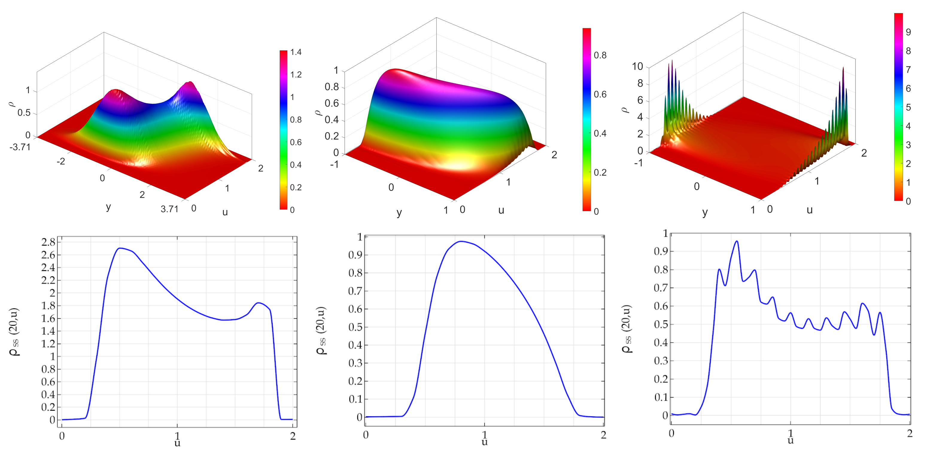
First, in Figure 1 we show the SSBHFPE and the associated marginal steady state distribution in the case where the bounded noise acts on the linear term of the logistic equation defining the activity of agents. In the left panels it is shown the ATAN case. The SSBHFPE (Upper left panel) is in this case characterized by two modes that, are asymmetric with respect to the noise-related variable y. This is surprisingly since the adopted stochastic perturbation is symmetric. In the lower left panel, we can observe again bimodality. Since the distribution of the model in absence of generation/destruction has a unique deterministic equilibrium at $u=1$ equal for all agents, this means that (adopting the terminology introduced in [55]) the bounded stochastic symmetric perturbation has induced a noise-induced-transition. In the central panel it is shown the impact of DCLpos noise: the PDF is a curved surface apparently convex everywhere but again it is asymmetric with respect to y despite the symmetric nature of the bounded stochastic perturbations. Finally, the right panels shown the impact of DCLneg noise. The bidimensional PDF is strongly asymmetric and it is characterized by a large number of peaks. The related marginal PDF (see right lower panels) is also multimodal and, roughly speaking, its envelope is reminiscent of the marginal distribution obtained in the case of arctan noise. In other words, also in this case NIT occurred. None of PDFs is symmetric, neither w.r.t. u nor w.r.t. y.

Instead, in Figure 2 we show the steady state of the BHFP equation in the case where the bounded noise acts on the carrying capacity of the logistic equation defining the activity of agents. In other words, we study the case where the action of the symmetric bounded noise is nonlinear. In the left panels it is shown the ATAN case. The SSBHFPE is in this case is unimodal with a portion fairly flat. The associated marginal PDF is unimodal and its mode is remarkably smaller than one. In the central panel it is shown the impact of DCLpos noise: the PDF is a curved surface. The associated marginal distribution is unimodal and its mode is at about $0.8$. Finally, the right panel shows the impact of DCLneg case: the PDF is strongly asymmetric and characterized by a large number of peaks. The associated marginal PDF has a large number of small peaks, but its envelope is reminiscent of a unimodal PDF, where the mode is about at $u=0.2$. None of PDFs is symmetric, neither w.r.t. u and y. All the SSBHFPE are strongly asymmetric w.r.t of both u and y.

12. Numerical Solution of the Full Birth Death System

In this section, we investigate the dynamics of the full birth death kinetic system by assuming as initial conditions the steady state solutions of the bidimensional hypoelliptic Fokker–Planck equation described in the previous section.

12.1. Noise Acting Linearly

In this subsection we consider the impact of a bounded noise acting on the linear term of the logistic equation.

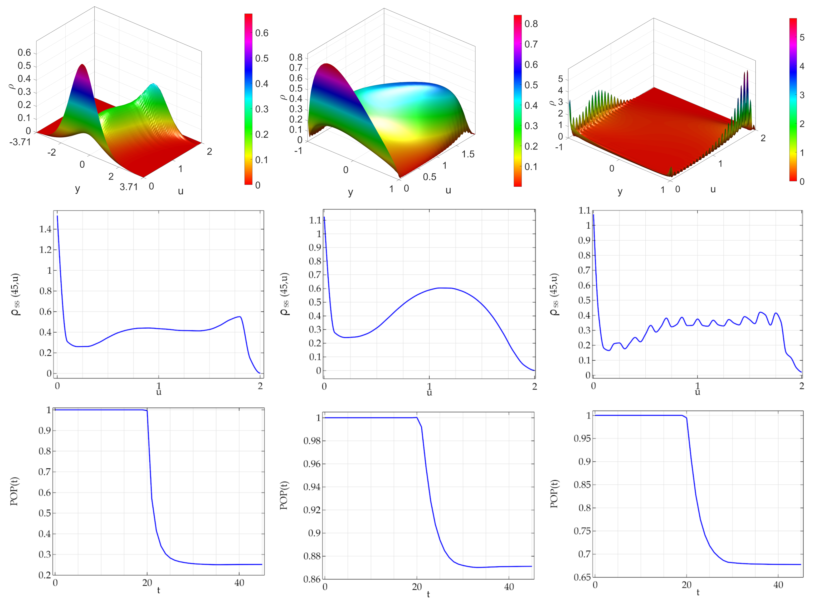
In Figure 3, it is shown the case where the mean of the activity of daughter agents is located at the activity of mother agent (w). As far as the bidimensional steady state densities, a new mode at zero is observed for both the ATAN and the DCLpos cases. As far as the marginal distributions is concerned, for all three types of noises that we considered the density of the population has a mode at zero. This implies that in the DCLpos case the birth and death terms implied the onset of a noise induced transition. Interestingly, although the birth and death terms are the same for all the three series of simulations, there is a remarkable quantitative difference in the steady state value of the population: the arctan noise is associated to a two steady state population, equal to about $0.3$. In the DCLpos case the steady state population is about $0.87$, whereas for DCLneg noise the steady state population is about $0.67$.

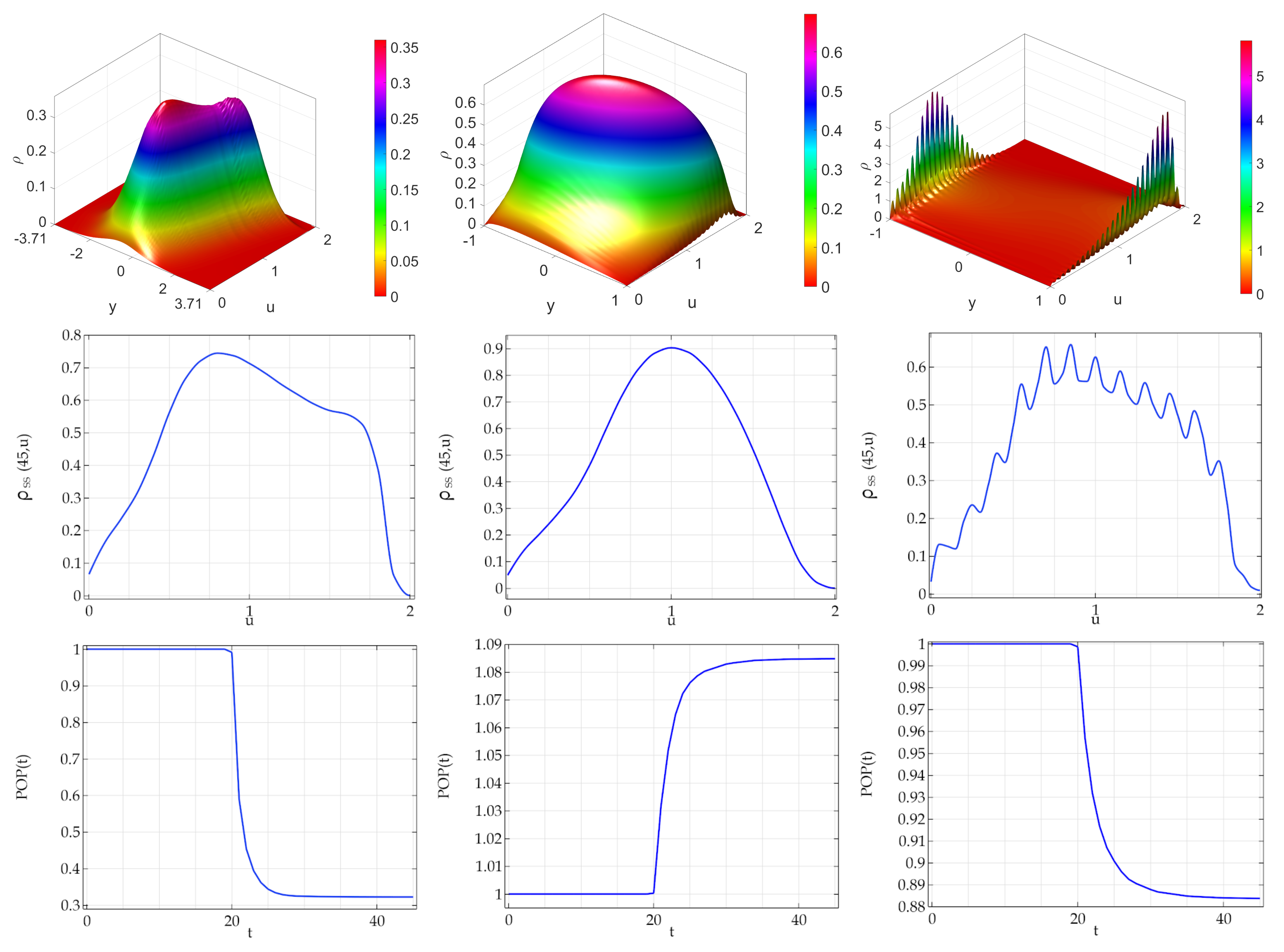
In Figure 4, it is shown the case where the mode of the activity of daughter agents is located at the activity of mother agent (w). As far as the steady state bidimensional densities, they are: (i) bimodal for the ATAN case but associated to a unimodal marginal density; (ii) unimodal for the DCLpos case; (iii) multimodal characterized by a large number of peaks for DCLneg noise. As far as the population dynamics we observe, quite interestingly, that in the DCLpos case about a $10\%$ increase of the population is observed.

12.2. Noise Acting Nonlinearly

In this subsection we consider the impact of a bounded noise acting on the carrying capacity term of the logistic equation, i.e., acting nonlinearly.

In Figure 5, (mean value of the daughter agents’ activities at the activity of the mother agent) we note that: (i) the ATAN case is characterized by trimodality in both the bidimensional and the marginal steady state densities, with one mode at zero; (ii) The DCLneg is characterized by a multi peaks strongly asymmetric bidimensional steady state density to which it is associated a trimodal like (plus manu local peaks) steady state density (iii) the DCLpos case is characterized by a curve bidimensional steady state density associated to a unimodal marginal density. As far as the dynamics of the total population, and in the previous subsection, the DCLpos case shows a moderate increase of the steady state value.

In Figure 6 (mode of the daughters agents’ activities at the activity of the mother agent) we note that (i) both in ATAN and in the DCLpos cases the bidimentional and the marginal densities are unimodal; (ii) as usual the DCLneg case is characterized bu a large number of peaks asymmetrically distributed. The most interesting phenomenon concerns the total population: here not only it is observed the 10% of increase previously observed, but also in the case ATAN a increase of the steady state population, and this increase is large: the 30%.

13. Impact of the Death and Birth Rates

Int their section we numerically show and example of the impact of both the birth and the death rates. Namely we set:

$$\alpha \left(N\right)=\frac{{\alpha }_0}{1+{\alpha }_1{N}^b};$$

(32)

$${\mu }_0\left(u\right)=1-\xi H(u-0.9);$$

(33)

$${\mu }_1\left(u\right)=0.5{\mu }_0\left(u\right).$$

(34)

As shown in Figure 7, which for the sake of the simplicity refers only to the ATAN case, the one system dynamics impact of the type of birth rate and of the parameter $\xi$ is remarkable, as it was expected.

14. Concluding Remarks

In this work, we considered a system of active particles, i.e., of agents (such as cells, animals in a flock, etc.) endowed by an internal variable u whose evolution is known and stochastic. Namely we assume that the dynamics of u is ruled by a nonlinear dynamical systems perturbed by realistic bounded symmetric stochastic perturbations: $u^{\prime }=f(u,p\left(t\right))$ where the dependence of the rhs on p can be nonlinear. In absence of birth and death of the agents the system evolution is ruled by a multidimensional hypo-elliptical Fokker–Plank equation.

However, we assume that each individual agent can reproduce by generating other agents whose activity is a stochastic variable related to the activity of the mother, animals in a flock. The agents can die. Both birth and death depend on the available resources, i.e., on the whole population. The resulting model is thus an Partial Integro-differential Equation with hypo-elliptical terms. If also a white noise perturbation act on agents, $u^{\prime }=f(u,p\left(t\right))+g\left(u\right)\xi \left(t\right)$, then the resulting model is a FPE with fully elliptical terms.

In the numerical simulations we focus on a simple case where the unperturbed dynamics of the agents is of logistic type and then we consider the presence of bounded symmetric stochastic perturbations acting in a linear and non-linear way. As far as the bounded perturbations are concerned, we consider the Doering–Cai–Lin noise and a new bounded noise, obtained by applying and arctan function to the well known Orenstein–Uhlenbeck Gaussian noise. We then numerically find the evolution and the steady state of the above—mentioned hypo-elliptical bidimensional Fokker–Plank equation to be used as initial state for the system in study.

We observed a number of phenomena that depends on the type of noise and on the interplay between noise and birth and death of agents.

First, since the unperturbed model in absence of birth and death has a unique equilibrium at $u=1$ (monostability), and since in both ATAN and DCLneg cases the bidimensional and the marginal densities are multimodal, this means that the bounded symmetric perturbations can induce noise induced transitions. However, this occurs (in our simulations) only in the case where the noise perturbs the linear term of the logistic equation.

The presence of the birth and deaths may induce, in turn; transitions from unimodality to bimodality even when the steady state of the FP equation is unimodal.

Moreover the total population can be in some cases quantitatively and qualitatively (decreasing vs. increasing time patterns) influenced in a noise-depending manner.

An important effect observed could be roughly described as a symmetry to asymmetry effect since despite the symmetric nature of the stochastic perturbations in some cases the distribution is asymmetric.

Finally, although in our simulations we did not find genuine phase transitions, notwithstanding that we pointed out that the nonlocality could result in some specific models in the onset of first or second order phase transitions.

Limitation and Specificity This study, eminently theoretical, has a number of limitations, real and apparent. The first and most important limitation is that here we study a prototypicalgeneric population of agents that is not directly derived by a specific biological problem. However, this is not a so strong limitation because we apply general principles common to many areas of cellular biology and ecology. Thus, this study could be classified as statistical biophysics/biomathematics inspired by biology.

The key novelty here is the fact that our multiscale mean field model explicitly included the presence of realistic bounded stochastic perturbations. This kind of stochastic perturbations have two classes of advantages. The first, largely discussed in the literature on bounded stochastic processes, is that bounded noises preserves the positivity of the parameters and impeded their excessive expansion. The second is that, at variance with white or colored Gaussian perturbations, even parameters that nonlinearly impact on the system can be perturbed.

The second limitation is that the proposed model is a mean field model. Furthermore, here two observations are useful to mitigate the nature of limitations. First, we qualitatively describe a problem that easily could be implemented by means of an individual based model. However populations of some types of agents such as cells rarely are of small medium size, and most often are of very large huge sizes, for which a mean field description are the one we propose here is well suited.

A third limitation is that we have chosen, for the sake of the simplicity, to focus on the behavior of a single population. However, also in this case intra-population interactions are biologically observed, leading to complex integro-differential terms in our model. the inclusion of multiple interplaying population can be easily be integrated by following the large body of research by Belomo and coworkers.

A final limitation is the use of bounded activities. The case of unbounded activities is important for two reasons: (i) this allows in a straightforward way the inclusion of the space is straightforward, since position and velocity it can be considered as a component of a generalized vectorial activity u; (ii) this could allow the possibility of the onset of traveling waves and solutions, a key topic in theoretical and applied mathematical physics [30,78,79,80,81,82] that have extremely interesting synergies with possible noisy perturbations [83].