Article

Symmetric and Asymmetric Diffusions through Age-Varying Mixed-Species Stand Parameters

by
Petras Rupšys
1,2,* and
Edmundas Petrauskas
2
1
Faculty of Informatics, Vytautas Magnus University, Studentų Str. 11, LT-53361 Kaunas, Lithuania
2
Agriculture Academy, Vytautas Magnus University, Studentų Str. 11, LT-53361 Kaunas, Lithuania
*
Author to whom correspondence should be addressed.
Symmetry 2021, 13(8), 1457; https://doi.org/10.3390/sym13081457
Submission received: 5 July 2021 / Revised: 22 July 2021 / Accepted: 30 July 2021 / Published: 9 August 2021

Abstract

:
(1) Background: This paper deals with unevenly aged, whole-stand models from mixed-effect parameters diffusion processes and Voronoi diagram points of view and concentrates on the mixed-species stands in Lithuania. We focus on the Voronoi diagram of potentially available areas to tree positions as the measure of the competition effect of individual trees and the tree diameter at breast height to relate their evolution through time. (2) Methods: We consider a bivariate hybrid mixed-effect parameters stochastic differential equation for the parameterization of the diameter and available polygon area at age to ensure a proper description of the link between them during the age (time) span of a forest stand. In this study, the Voronoi diagram was used as a mathematical tool for the quantitative characterization of inter-tree competition. (3) Results: The newly derived model considers bivariate correlated observations, tree diameter, and polygon area arising from a particular stand and enables defining equations for calculating diameter, polygon-area, and stand-density predictions and forecasts. (4) Conclusions: From a statistical point of view, the newly developed models produced acceptable statistical measures of predictions and forecasts. All the results were implemented in the Maple computer algebra system.

1. Introduction

Forest statisticians often need to address complex issues in important whole-stand, unevenly aged growth models with high levels of uncertainty that affect individual trees. Providing scientific evidence for effective decision processes in forest areas is a key issue, and stochastic calculus is an essential tool [1].
In the past few decades, mathematical models based on diffusion processes were fruitfully applied to describe stochasticity phenomena belonging to even extremely different disciplinary fields that range in scale from human population in biology [2] to cryptocurrency in finance [3] and from infectious disease in medicine [4] to networks in neuroscience [5]. Mixed-effect parameters diffusion processes provide a convenient tool to account for differences between several experiments or several subjects [6].
One of the important aims of modern forest regeneration is the investigation of the mapped tree community distribution in a stand area and its evolution through time. The distribution of individual trees depends both on the initial conditions present in a forest stand and the successive development of trees through changes in size components and mortality events. At present, results are large datasets of observations and statistical analysis acquired by using competition indices to both direct and indirect stand measurements [7]. To operate with these data, it is necessary to investigate information in a convenient form for the mathematical modeling of individual-based tree growth and yield. Independently of the type of an individual tree or whole-stand stochastic modelling (having a random variable), the consideration of a diffusion process has particular challenges. Diffusion processes allow for us to compute both the solution of the corresponding stochastic differential equation in a form of probability density function and their statistical moments, mainly mean, quantiles, and variance. The mechanism of the evolution of the competition among living trees in a forest stand can be successfully described by using a relatively young mathematical tool—continuous stochastic differential equations (SDEs). SDEs serve the purpose of analysis in a wide variety of generic growth models with different resolutions. The most advanced statistical models of this kind were formulated in terms of multivariate diffusion processes [8].
The process by which tree seedlings start to grow successfully in a new place is spatially multivariate, with numerous unknown variables. A potentially available area for an individual seedling embodies a variable representing the competitive strength of individual tree–tree interactions and varies through time. Several case studies were conducted to study the relationships between the potentially available area of a tree and its main biometrical attributes and competition indices [9]. The competition index is widely applied in plant ecology, but it has a smaller number of applications in individual-tree or whole-stand modeling. From a mathematical point of view, the Voronoi diagram [10] can be regarded as the best solution for neighboring effects on tree-size growth. To illustrate this study, we use the Voronoi diagram method, which is used by the individual-based tree-growth model. The Voronoi diagram formalizes a detailed structure of the position, size, and shape of a potentially available area of individual trees with respect to the number of trees per unit area and nearness of their contiguous neighbors. Moreover, Voronoi polygons reflect the local variation of the number of trees in a given location. A variable outlined by the value of the area of the Voronoi polygon is used as a descriptive parameter of spatial arrangement and as a predictor of stand density models.
Almost all the published research on natural mechanisms of maintaining tree-species diversity focuses on the principles of spatial measures and competition-index construction and their biological and mathematical reasoning [9]. Previous relationships on the key competition index include only local neighbors and are static. Unfortunately, it is insufficient, as each competition index systematically changes through time, which is of great importance and highly correlated with tree-size variables. Therefore, this paper focuses on the Voronoi polygon area of a tree and its dynamics. The dynamics of the polygon area is described by a diffusion process that accounts for the competition effect of contiguous neighbors and its correlation with tree-size or -stand variables.
This paper deals with whole-stand models from a diffusion process of view and concentrates on mixed-species stands in Lithuania. The innovation of this paper lies in the following: (1) the Voronoi diagram of potentially available areas to tree positions as the measure of the competition effect of individual trees, and its evolution through time is described using a Gompertz-type diffusion process; (2) the link of stand density with potentially available area and tree diameter is analyzed; (3) the mean and quantile attribute equations of the potentially available area, tree diameter, and stand density are described; and (4) the significance of differences in the distributions of different tree species is assessed. This paper carries out further research from the following directions: the first aspect analyzes the stochastic fixed-effect parameters process and then the stochastic mixed-effect parameters process; the third aspect illustrates the computational properties of the derived models.
The study was conducted in naturally and artificially regenerated areas by using data collected from over 58,000 trees positioned in a network of 50 permanent, rectangular sampling plots. As significant variables in the present study, we used such assessed attributes as species, the location of the individuals (Cartesian coordinates x, y), tree diameter at 1.3 m above ground level, and age. In order to determine the individual area of the i-th (i = 1, …, n) tree, Voronoi polygon area Pi was calculated.
By utilizing the additive and multiplicative noise systems, we define the hybrid bivariate Vasicek–Gompertz-type SDE. The inclusion of random effects in the SDE produced a more accurate model to account for the error between model predictions and observed dataset. Model building in forestry was traditionally formalized by empirical models supporting the decisions of forest managers [11]. In addition, large published growth and yield systems were described by regression analysis, developed on a statistical basis that actually sought only to highlight the importance of a particular response variable in predicting the future, remaining static and deterministic. The stochastic differential equation approach opened the way to a stochastic dynamical formulation of the individual-tree or whole-stand growth process that appeared much later in statistical forestry [12,13,14].

2. Materials and Methods

2.1. Voronoi Diagram

Considering data in the form of a given set of n points (xi; yi), i = 1, …, n within a planar region A, we can assign an area to (xi; yi) consisting of that part of A that is closer to (xi; yi) than to any other point (xj; yj). A Voronoi diagram involves the partitioning of a planar region A into regions or polygons Ai on the basis of the distance to a specified discrete set of points [15]. The Voronoi diagram is a mathematical tool for the quantitative characterization of natural phenomena, such as inter-tree competition. In these polygons, trees with which the area neighbors are in direct competition for available light and nutrients are shown [16]. Each area Ai is a convex polygonal region. Voronoi polygons Ai vary with increasing time, and the number of trees decreases. Considering the dynamic of the Voronoi diagram allowed for both the quantification of its temporal dynamics and the characterization of the number of trees in a stand and its dynamics through time.
A generic definition of Voronoi diagrams was mathematically first introduced by Aurenhammer [17]. Voronoi cell Ai, associated with point (xj; yi), is the set of all points in A, of which distance to point (xj; yi) is not greater than their distance to other point (xj; yj), where j is any index different from i. If we assume that d((x; y),B) = inf{d((x; y),(a1; a2))|(a1; a2) ∈B} denotes the distance between point (x; y) and subset B, then:
A i = ( x ; y ) A | d ( x ; y ) ,   A i d ( x ; y ) ,   A j   f o r   a l l   j     i .
The Voronoi diagram is simply the corpus of polygons Ai, i = 1, …, n. In the past decade, mathematical algorithms and the rapid development of computational capacities provided a new chance to develop Voronoi diagram-based applications. In this study, we discuss mathematical models and their analyses based on areas of generated Voronoi polygons. To illustrate our work, we computed the Voronoi polygon of each individual tree in a plot, which was remeasured four times and is visualized in Figure 1, which shows that the areas of the Voronoi cells change through age (time).

2.2. Bivariate SDEs of Diameter and Polygon Area

In forestry studies, most tree attributes are considered to be functions of the tree diameter at breast height D [18]. For explaining the dynamics of tree-size variables, the incorporation of the distance of neighboring trees into a model improves predictions [19]. Moreover, appropriate evaluation of individual-tree size-variable is a fundamental requirement for the analysis of stand variables, such as the number of trees and volume per hectare. This study considers a stochastic approach for the parameterization of diameter D and polygon area P at age to ensure the proper descriptions of their link during the age (time) span of a forest stand. In this section, we state the stochastic mixed-effect bivariate (diameter D and polygon area P) model and derive the corresponding bivariate probability density function. We also introduce the procedure for random-effect calibration. The Vasicek–Gompertz-type bivariate hybrid stochastic mixed-effect parameters model was used to parameterize diameter and polygon area at age-discrete data. The univariate Gompertz-type model was applied to the analysis of stem volume and tree-stem taper from different tree species [20]. Below, stochastic vector X i t = X 1 i t , X 2 i t T = D i t , P i t T , i = 1,…,M, t t 0 ; T , M is the number of individuals (plots), and T is a finite horizon, T < ∞. Hybrid bivariate Vasicek–Gompertz-type SDE is defined as:
d X i t = A i X i t d t + D X i t B 1 2 d W i t P X i t 0 = x 0 = 1 ,   i = 1 ,   ,   M ,
A i x = β d α d + φ d i x 1 , α p + φ p i β p l n ( x 2 ) x 2 T B = σ d d σ d p σ d p σ p p ,
D x B 1 2 D x B 1 2 T = 1 0 0 x 2 σ d d σ d p σ d p σ p p 1 0 0 x 2
This study focusses on initial distribution, defined by deterministic initial value X 1 i t 0 , X 2 i t 0 = ( x 10 , x 20 ) = x 10 , δ + φ 0 i , and δ is an unknown fixed-effect parameter to be estimated. SDE of form (2) consists of two parts. The deterministic part in the model is drift function A i x . Random term D X i t B 1 2 d W i t , which corresponds to the uncertain part of the model, is referred to as the system noise. In Equation (2), W i t = W 1 i t , W 2 i t T represents the bivariate Brownian motion, of which the time derivative is white noise. Moreover, Brownian motion increments d W i t , i = 1,…,M, are considered to be independent across all plots. Random effects φ d i φ p i , and φ 0 i are independent and normally distributed random variables with zero mean and constant variances, respectively, φ d i ~ N 0 ; σ d 2 , φ p i ~ N 0 ; σ p 2 , and φ 0 i ~ N 0 ; σ 0 2 . Fixed-effect parameters vector θ to be estimated is defined as:
θ = α d ,   α p , β d , β p , σ d d ,   σ p p , ρ d p , δ , σ d , σ p ,   σ 0 σ d p = σ d d σ p p ρ d p .
The solution of the Vasicek–Gompertz-type SDE (2) has bivariate normal-lognormal distribution N 1 L N 1 μ i ( t | t 0 , x 0 ) ; Σ ( t | t 0 ) with mean vector μ i ( t | t 0 , x 0 ) and variance–covariance matrix Σ ( t | t 0 ) , defined as:
μ i t | t 0 , x 0 = μ d i t | t 0 , x 10 μ p i ( t | t 0 , x 20 ) = ( α d + φ d i ) + x 10 ( α d + φ d i ) e β d ( t t 0 ) e β p ( t t 0 ) l n ( δ + φ 0 i ) + 1 e β p ( t t 0 ) β p α p + φ p i σ p p 2
Σ t | t 0 = v d d t | t 0 v d p ( t | t 0 ) v d p ( t | t 0 ) v p p ( t | t 0 ) = 1 e 2 β d t t 0 2 β d σ d d 1 e β d + β p t t 0 β d + β p σ d d σ p p ρ d p 1 e β d + β p t t 0 β d + β p σ d d σ p p ρ d p 1 e 2 β p t t 0 2 β p σ p p .
We can separately calculate the probability distribution of each random variable if we wish to restrict our attention to the value of just one, for example, diameter D or polygon area P. The marginal distribution of X 1 i t | X 1 i t 0 = x 10 is normal N 1 μ d i ( t | t 0 , x 10 )   ; v d d t | t 0 , and the marginal distribution of X 2 i t | X 2 i t 0 = x 20 is lognormal L N 1 μ p i ( t | t 0 , x 20 )   ; v p p ( t | t 0 ) with means μ d i ( t | t 0 , x 10 ) and μ p i ( t | t 0 , x 20 ) and variances v d d t | t 0 and v p p t | t 0 , respectively.
For the diameter dynamic, the mean, median, mode, qth quantile (0 < q < 1), and variance trends can be listed as:
m d i t | t 0 , x 10 = m e d i t | t 0 , x 10 = m o d i t | t 0 , x 10 = μ d i ( t | t 0 , x 10 ) ,
m q d i t , q | t 0 , x 10 = Φ q 1 μ d i t | t 0 , x 10 ; v d d t | t 0 ,
w d i t | t 0 , x 10 = v d d t | t 0 ,
where Φ q 1 ; is the inverse of the standard normal distribution function.
For the polygon area dynamic, the mean, median, mode, qth quantile (0 < q < 1), and variance trends can be listed as:
m p i t | t 0 , x 20 = e x p μ p i ( t | t 0 , x 20 ) + 1 2 v p p t | t 0 ,
m e p i t | t 0 , x 20 = e x p μ p i ( t | t 0 , x 20 ) ,
m o p i t | t 0 , x 20 = e x p μ p i t | t 0 , x 20 v p p t | t 0 ,
m q p i t , q | t 0 , x 20 = L Φ q 1 ( μ p i ( t | t 0 , x 20 ) ; v p p t | t 0 ) ,
w p i t | t 0 , x 10 = e x p 2 μ p i ( t | t 0 , x 20 ) + v p p t | t 0 exp v p p t | t 0 1 ,
where L Φ q 1 ; is the inverse of the standard normal distribution function.
Conditional distribution of X 1 i t | X 1 i t 0 = x 10 at a given X 2 i ( t ) = x 2 is univariate normal N 1 η d i ( t , x 2 | t 0 , x 0 ) ; λ d ( t | t 0 ) , and conditional distribution of X 2 i t | X 2 i t 0 = x 20 at a given X 1 i t = x 1 is univariate lognormal L N 1 η p i ( t , x 1 | t 0 , x 0 ) ; λ p ( t | t 0 ) , with means and variances given as:
η d i t , x 2 | t 0 , x 0 = μ d i ( t | t 0 , x 10 ) + v d p t | t 0 v p p t | t 0 ln x 2 μ p i ( t | t 0 , x 20 )  
λ d t | t 0 = v d d t | t 0 v d p t | t 0 2 v p p t | t 0 ,
η p i t , x 1 | t 0 , x 0 = μ p i ( t | t 0 , x 20 ) + v d p t | t 0 v d d t | t 0 x 1 μ d i ( t | t 0 , x 10 ) ,
λ p t | t 0 = v p p t | t 0 v d p t | t 0 2 v d d t | t 0 .
For the diameter growth model, the conditional mean, median, mode, qth quantile (0 < q < 1), and variance trends can be listed as:
m c d i t , x 2 | t 0 , x 0 = m e c d i t , x 2 | t 0 , x 0 = m o c d i t , x 2 | t 0 , x 0 = η d i t , x 2 | t 0 , x 0 ,
m q c d i t , x 2 , q | t 0 , x 0 = Φ q 1 ( η d i ( t , x 2 | t 0 , x 0 ) ; λ d t | t 0 ) ,
w c d i t | t 0 = λ d t | t 0 .
For the polygon area growth model, the conditional mean, median, mode, qth quantile (0 < q < 1), and variance trends can be listed as:
m c p i t , x 1 | t 0 , x 0 = e x p η p i t , x 1 | t 0 , x 0 + 1 2 λ p t | t 0 ,
m e c p i t , x 1 | t 0 , x 0 = e x p η p i t , x 1 | t 0 , x 0 ,
m o c p i t , x 1 | t 0 , x 0 = e x p η p i t , x 1 | t 0 , x 0 λ p t | t 0 ,
m q c p i t , x 1 , q | t 0 , x 0 = Φ q 1 ( η p i ( t , x 1 | t 0 , x 0 ) ; λ p t | t 0 ) ,
w c p i t , x 1 | t 0 , x 0 = e x p 2 η p i t , x 1 | t 0 , x 0 + λ p t | t 0 e x p λ p t | t 0 1 .

2.3. Data

The field-study area is located in the municipality of Kazlų Rūda in Lithuania. A major part of the Kazlų Rūda municipality is located in the fertile Užnemunė lowland and is among the most wooded areas in Lithuania, with about 59.4% of the territory covered by large forests. The specific allocation comprises the area covered by stands of pine (Pinus sylvestris), 63.8%; spruce (Picea abies), 30.2%; silver birch (Betula pendula Roth and Betula pubescens Ehrh.), 5.8%; and others, 0.2%. All data were collected during fieldwork in 1983–2019 across the Kazlų Rūda forests (latitude, 54°44′54.222″ N; longitude, 23°29′27.7944″ E; altitude, 68 m). Mean temperatures vary from −16.4 °C in winter to 22 °C in summer. Precipitation is distributed throughout the year, although predominantly in summer; the average is approximately 680 mm a year. During the 1983–1987 period, 50 permanent experimental plots were established in the Kazlų Rūda forests in Lithuania. According to regeneration mode, the 50 field-sample plots vary between those naturally and artificially regenerated and spread in pure or mixed-species stands. Each sample plot consisted of about 0.16–0.72 ha and was remeasured several times, from 1 until 6 (see Figure 1, showing 4 cycles) at 2- to 36-year intervals. The attributes recorded for each tree in the considered plots were the tree species, age, location of the sample trees (planar coordinate position x and y), and diameter at breast height. The age of the i-th tree (i varied from all the trees until the 10th) in the first measurement was recorded by counting its growth rings on the increment core (for even-aged stands, from entries in documents), and the ages of the remaining trees were obtained from the arithmetic mean. The accuracy of planar coordinate position was 1 dcm, and diameter measurements were performed with approximately 1 mm accuracy. The 50 field-sample plot dataset was randomly divided into estimation and validation datasets. The estimation dataset consisted of measurements from 40 plots, and the validation dataset compounded the remaining measurements from 10 plots. Table 1 shows the summary statistics of the field-sample data.

3. Results

3.1. Parameter-Estimating Results

The key research problem in this study is the latest developments of accurate and computationally optimal parameter-estimation procedures based on the approximated maximum-likelihood technique, which cannot be implemented in the presence of a closed-form expression for the mixed-effect parameters SDE [21]. Our developed maximum-likelihood estimation technique relies on the fact that the conditional bivariate probability density function has an exact form. Therefore, the likelihood function maximization technique with respect to parameter vector θ for a given set of discretely observed diameter and polygon area data is defined by a two-step procedure.
To evaluate the proposed Vasicek–Gompertz-type mixed-effect parameters SDE (2), an approximated log-likelihood technique for estimating the parameters was set up on the basis of the discrete observations from estimation dataset d 1 i , p 1 i , d 2 i , p 2 i , , d n i i , p n i i on a fixed time interval t 1 i , t 2 i , , t n i i ,  i = 1,…,M. The randomly selected 40 samples were used to fit the SDE model defined by Equation (2), and the results of the estimating parameters are summarized in Table 2. All parameters were statistically significant (p < 0.05).

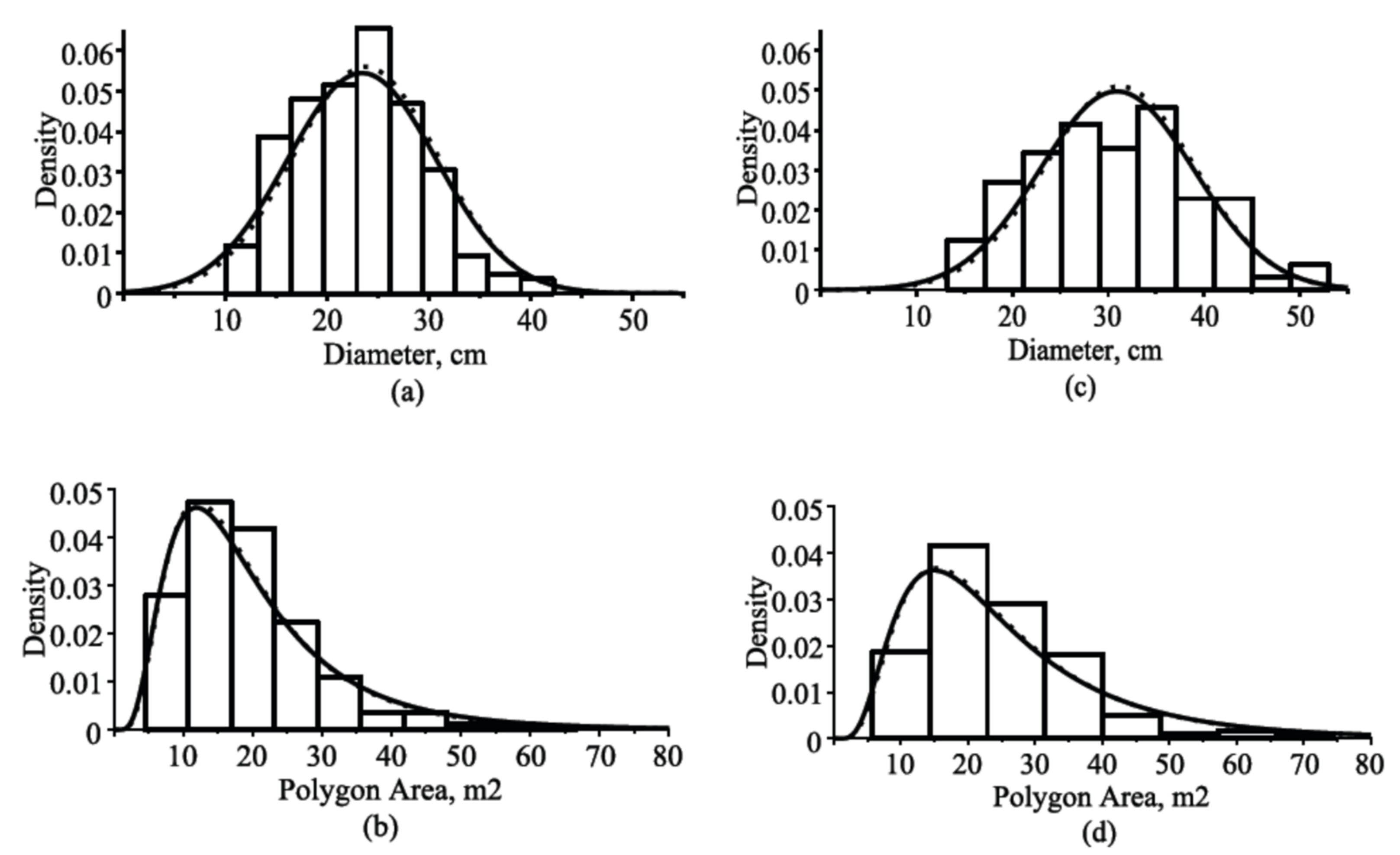
3.2. Bivariate and Marginal Distributions

After the fixed-effect parameters were obtained in Section 3.1, which are listed in Table 2, they were used to evaluate the accuracy of the prediction and forecasting in subsequent sections by using data from the validation dataset. The bivariate mixed-effect parameters SDE model was developed by combining the two univariate models through a bivariate stochastic process. The model considered two correlated observations, tree diameter and polygon area, reflecting the high variation of stand density among stands of Lithuania. The main goal in an SDE modeling framework is to determine the probability density function of the solution, formulated as a diffusion process since it capacitates for calculating any univariate moment, which allows for calculating the mean, variance, and tolerance regions for bivariate cases. In our setting, the newly developed bivariate density and marginal and conditional densities were visually evaluated corresponding to the diameter and polygon area observed data from the validation dataset at a given average stand age. Therefore, the corresponding observed data from the validation dataset and its fitted distribution were graphically visualized. The Voronoi tessellations presented in Figure 1 show dynamic of polygon areas via stand age (time). These diagrams also demonstrate information about variations in the polygon area, which grows with age. Figure 2, Figure 3, Figure 4 and Figure 5 illustrate the fitted marginal probability density functions and underlying frequency distributions (histograms) for new plots from the validation dataset with two cycles of remeasurements at an average stand age. All the fitted probability density functions take the values of the fixed-effect parameters from Table 2. Random effects φ d , φ p , and   φ 0 for a new plot from the validation dataset were calibrated as:
φ = a r g m a x φ d , φ p , φ 0 j = 1 m l n f x 1 j , x 2 j , t j θ , φ d , φ p , φ 0 + l n ϕ ( φ d σ d ) + l n ϕ φ p σ p + l n ϕ φ 0 σ 0
where x 11 , x 21 , x 12 , x 22 , , x 1 m , x 2 m is the newly observed dataset, t0 = 4, x 10 , x 20 = 0.1 , δ ^ + φ 0 , f x 1 , x 2 , t θ 1 , φ d , φ p , φ 0 is the bivariate normal-lognormal density function with the mean and variance defined by Equations (5) and (6), ϕ ( · σ ) is the univariate normal density function with zero mean and standard deviation σ, and the estimated values of fixed-effect parameters are denoted by “hat” (listed in Table 2).
Figure 2, Figure 3, Figure 4 and Figure 5 show that univariate conditional probability density functions defined by inserting additional explanatory variable polygon areas or diameters undergo indistinguishable changes in comparison with corresponding univariate marginal densities. The similarity of the marginal and conditional distributions suggests that the additional explanatory variable (polygon area or diameter) has a relatively small effect on the values of the response variable (diameter or polygon area). Moreover, the figures superpose frequency distribution and estimated normal or lognormal probability distributions that correspond to the probability density function of the solutions of SDE (2). Frequency distributions are not exactly in agreement with the normal or lognormal distribution shapes due to the variation in tree age or probably did not arise from our presented form. The tree diameter histograms shown in Figure 2, Figure 3, Figure 4 and Figure 5 confirm the assumption that the tree-diameter distribution in a particular forest stand has an approximately symmetrical shape. The lack of symmetry in Figure 4 for Norway spruce trees occurs probably due to the planned thinning in the stand, as lightening works are usually carried out in stands of this age. The symmetry and standard deviation of the diameter distribution increase with age. In contrast, the polygon area histograms reveal asymmetry of the distribution, and the long tail extends to the right. Histograms of the polygon area show a number of unusual observed values. This scenario may be the result of a directional felling or soil properties. Lastly, the newly derived bivariate probability density function was a good match for our validation data.
For the observed diameter and polygon area data fitted with the bivariate Vasicek–Gompertz-type SDE (2), the tolerance region of mean vector μ i ( t | t 0 , x 0 ) , defined by Equation (5), takes the following well-known inequality [22]:
x 1 l n x 2 μ i t | t 0 , x 0 T Σ t | t 0 1 x 1 l n x 2 μ i t | t 0 , x 0 χ ,
where x is the tolerance coefficient [23]. For lognormally distributed polygon area data, we plot a tolerance region using a logarithmic axis. Figure 6, Figure 7, Figure 8 and Figure 9 show the tolerance regions for β = 0.95 and confidence level γ = 0.95, which correspond to the randomly selected stand from the validation dataset with two cycles of remeasurements. The random effects were calibrated by Equation (27). For the tolerance region plots, the x value was chosen from Table 1 in [23]: the setting β = 0.95 and γ = 0.95 produces a x of 10.02. The bivariate tolerance region for the Vasicek–Gompertz-type model (2) enables us to decide whether the newly developed distribution function corresponds well with the observed data of the diameter and polygon area. Figure 6, Figure 7, Figure 8 and Figure 9 illustrate that the 95% tolerance regions had reasonable coverage rates for different tree-species scenarios. Information concerning tolerance regions is implicit in the hybrid bivariate distribution derived for the Vasicek–Gompertz-type SDE (2).

4. Discussion

Figure 2, Figure 3, Figure 4 and Figure 5 show that very high variation existed in the shape of the diameter and polygon area frequency distributions among plots of a given stand age. In our models, this variation was well accounted for by the used diffusion process defined by SDE (2). Since the observed sample plots represent forest stands in the region, the plot effects were generally included by using three random variables (effects). To properly test our mixed-effect model of diameter, polygon area, and number of trees per hectare, we used observed sample plots from the validation dataset to show its robustness in predicting (via current age) and forecasting (future age).

4.1. Modeling Tree-Diameter Dynamics: Predicting and Forecasting

Traditionally, individual-tree-diameter-growth regression models describe growth as a function of an age (tree or stand). Most individual-tree-diameter-growth models were framed using an algebraic difference approach [24] and its mathematical generalizations [25]. The SDE (2) developed in this study enables us to describe a wide range of tree- and stand-growth variables. To apply the mixed-effect SDE model defined by Equation (2), we had two adaptation strategies—prediction and forecasting. First, the underlying random effects of the model were precisely calibrated (using all remeasurement cycles from the validation dataset). Hence, random effects were calibrated by Equation (27) using data from the validation dataset in order to define the predictions (dynamic against the age) of the mean, variance, and quantiles of the diameter or polygon area in a particular stand. In this strategy, we could average the results of multiple realizations of tree diameters in different plots and obtain important characteristics (mean and variance) that could not be seen in one tree realization. Second, the underlying random effects of the model were not precisely calibrated (using only the first measurement cycle in a plot). Hence, random effects were calibrated by Equation (27) using measurements of diameter, polygon area, and age at the initial measurement cycle from the validation dataset in order to define the forecasts, at the 5-, 13-, and 35-year forecast periods, of the diameter or polygon area for each individual tree. Most remeasured plots from the validation dataset were unevenly aged and mixed-species. Figure and table illustrations are separately presented for all tree species, Scots pine tree species, Norway spruce tree species, and silver birch tree species. Figure 10 shows predictions of the mean diameter, 0.05 and 0.95 quantiles for all, Scots pine, Norway spruce, and silver birch tree species for two randomly selected stands from the validation dataset.
The mean prediction error (percentage of prediction error, %) B, mean absolute prediction error (percentage of absolute prediction error, %) AB, root-mean-square error (percentage of root-mean-square error, %) RMSE, and coefficient of determination R2 were used to evaluate the results of the mean diameter-marginal and conditional model fit defined by Equations (7) and (19), respectively. The calculated results of statistical measures using the validation dataset, the fixed-effect parameters from Table 2, and random effects calibrated by Equation (27) are presented in Table 3. The prediction performance of both models (marginal and conditional) showed that both models were highly capable of identifying the mean value of the diameter in a stand. Subsequently, only a small improvement in the statistical measures was found when we used the polygon area as an additional explanatory variable (conditional model (19)). Table 3 illustrates the accuracy of mean diameter predictions by using the observed validation dataset.
The marginal and conditional models defined by Equations (7) and (19) can also be used successfully as individual-tree-based models in forecasting tree growth regardless of species, age, and tree polygon area. In Equation (7), if initial point x 10 , x 20 = 0.1 , δ ^ + φ 0 i was changed by point x 10 , x 20 = d i n , j i , p i n , j i + 0 . ,  i = 1,…,K (K is the number of the observed sample plots from the validation dataset), we could calculate forecasts of individual-tree diameters and compare them with the observed dataset by determining the duration of the forecast period (5, 13, and 35 years), where d i n , j i , p i n , j i is the diameter and polygon area of the j-th tree in the i-th plot at base age tin,j, and random effects φ d i φ p i and φ 0 i are equated to 0. Table 4 shows the forecast statistical measures of a tree-individual scenario model calculated for the 5-, 13-, and 35-year forecast periods using the fixed-effect parameters estimates in Table 2.
In general, the relative success of the 35-year forecast period in forecasting individual tree diameters showed that the values of statistical measures were considerably smaller than statistical measures were for the 5- and 13-year forecast periods. Therefore, the shorter (5 and 13 years) forecast periods provided us with reasonably accurate forecasts of tree diameters but performed quite poorly farther into the future. Compared to different tree species, Norway spruce species produced the lowest value of all statistical measures.

4.2. Modeling Tree Polygon Area: Predicting and Forecasting

The tree polygon areas show spatial tessellation based on closeness to trees in a particular stand. It was suggested by mathematician Voronoi [10] and named after him: Voronoi polygons (diagrams). A particular forest stand is driven with occasional events, and the spatial tree arrangement in it is featured with complexity and variability. Most studied Voronoi polygons are only static. A first approach for the dynamization of Voronoi diagrams could be an investigation by a procedure for inserting and deleting single trees (points), each in linear time. In modeling real dynamic scenes of a particular forest stand, parallel continuous changes of trees with a fast update of the Voronoi diagram are desirable. Four realizations at different times of a Voronoi polygon in a particular stand are presented in Figure 1. The main result of the present work consists in the dynamization of the underlying Voronoi polygon areas by the Gompertz-type diffusion process. Figure 11 shows predictions of the mean polygon area and 0.05 and 0.95 quantiles for two randomly selected stands from the validation dataset. Random effects were calibrated by Equation (27) using measurements of tree positions from the validation dataset, and the fixed-effect parameters are from Table 2.
The results of statistical measures of polygon area predictions, calculated using tree positions from the validation dataset, the fixed-effect parameters from Table 2, and random effects calibrated by Equation (27), are presented in Table 5, which clarifies the importance of the diameter employed in the modeling process. The prediction performance of both models defined by Equations (10) and (22) showed that both models were highly capable of identifying the mean value of the polygon area in a plot. On the other hand, only small improvement in the statistical measures was found (up to 3% in the coefficient of determination) when we used diameter as an additional explanatory variable in the conditional model defined by Equation (22).
Statistical measures of forecasts of trees’ individual polygon areas using an observed validation dataset, the fixed-effect parameters from Table 2, and at random effects equal to zero, φ d i = 0 . ,   φ p i = 0 . ,   φ 0 i = 0 . , i = 1, …, K, are presented in Table 6 for the forecast periods of 5, 13, and 35 years. The conditional model defined by Equation (22) was evaluated using a data subset of diameters drawn from the validation dataset at the projected (forecast period) age and showed that the influence of diameters cannot greatly improve the forecast ability of a mixed-effect polygon area model. Statistical measures in Table 6 show that the accuracy of the model forecast decreases significantly with increasing the forecast period to 35 years.

4.3. Modeling Stand Density: Predicting and Forecasting

To manage the evolution of the number of trees per hectare from the early sapling stage to any stage in mixed-species, unevenly aged forests, reliable predictive and forecast models are needed. The complete size–density trajectory of a stand from an early development stage follows the form framed by the maximal size–density relationship [26]. Recently, diffusion processes were used to define maximal size–density equations [27]. Many various stand-density measures were developed as relationships of mean area available to trees in a particular stand [28,29]. The stand density expresses a stand occupancy in abstract form; consequently, in this study, the stand density per hectare dynamic is related to the dynamic of the polygon area, defined by Equations (10) and (22), in the following forms for all the tree species:
N i t | t 0 , x 20 = 10000 m 2 i t | t 0 , x 20 ,
N i t | t 0 , x 20 , x 11 = 10000 η 2 i t , x 11 | t 0 , x 0 ,
and for constituent tree species:
N i t | t 0 , x 20 = o c i n 10000 m 2 i t | t 0 , x 20 ,
N i t | t 0 , x 20 , x 11 = o c i n 10000 η 2 i t , x 11 | t 0 , x 0 ,
where o c i n is the occupation proportion of a specific tree species in a stand at an age of the first measurement (0 < o c i n < 1).
Sustainable forest management requires the comprehensive understanding of the long-term dynamics of stand density. The stand-density models defined by Equations (29)–(32) enable us to evaluate stand density in both prediction and forecasting scenarios. For calculating predictions of stand density, we used the fixed-effect parameters from Table 2 and the random effects calibrated by Equation (27), using a full validation dataset. Figure 12 shows the mean stand-density dynamics for all tree species and constituent tree species scenarios and compares with observed datasets for three randomly selected stands from the validation dataset. The accuracy measures of the mean stand-density predictions are presented in Table 7.
The Voronoi polygon of tree positions is a powerful tool for understanding the spatial competition properties on the basis of closeness to trees in a particular stand. Relatively few studies reported the construction of Voronoi polygons in forest-stand modeling [30] despite a wide array of potential applications. Dynamic Voronoi polygons have applications among stand-density models, as they can be used to accurately define the rate of natural mortality among trees within a forest. Results of diameter importance for stand-density modeling processes are shown in the conditional models defined by Equations (30) and (32), presented in Table 7, which shows that employing the diameter in the modeling process provided small improvement in statistical measures (up to 3% in the coefficient of determination).
In stand-density dynamic models, transition probability density functions only consider natural mortality that is influenced by competition, whereas general response functions account for the effects of the site index, basal area, and other factors [31]. The newly developed stand-density dynamic functions defined by Equations (29)–(32) were developed with the purpose of formalizing a whole-stand model for predicting and forecasting a given mixed-species forest stand. As such, the observed dataset (40 plots) from long-term remeasurements (from 1 until 6 cycles) of permanent plots was used to evaluate the fixed-effect parameters for both predicting and forecasting scenarios. Concerning the stand-density forecast scenario, the random effects for a new stand were calibrated by Equation (27) using the first measurement cycle observed sample from the validation dataset. Comparisons of stand-density forecasts (projections) among the forecast periods of 5, 13, and 35 years are presented in Table 8.
All the tested models for all the tree species provided good forecasts for data with high statistical measures. All the models for Scots pine, Norway spruce, silver birch, and all the tree species resulted in high coefficients of variation for the forecast periods of 5, 13, and 35 years in intervals of 96.6–98.2%, 89.1–93.8%, and 60.5–92.5%, respectively. Both scenario models for Scots pine trees were comparably better. Similar results were obtained in model ranking on the basis of B, B%, AB, AB%, RMSE, and RMSE%. Statistically, the marginal models defined by Equations (29) and (30) and the conditional models defined by Equations (30) and (32) provided similar forecasts for all forecast periods.

5. Conclusions

In this paper, we have studied the evolution of the mixed-species, unevenly aged forest stands by using a bivariate hybrid diffusion process and Voronoi diagram. The growth model considers two different system states (tree diameter and polygon area). In summary, derived individual-tree and whole-stand models describe how trees grow in diameter and how forest-stand structures are modified over time. On the other hand, one of the most fundamental features of our developed models is that they are strongly symmetrical, as they allow for forecasting trajectories in the future and the past. Numerical example by using experimental sample plots in Lithuania with measurements of tree position, age, and diameter at breast height showed high accuracy of the obtained results and the importance of the work. From a statistical point of view, the newly developed growth models produced acceptable predictions and forecasts. Our proposed bivariate hybrid diffusion process and Voronoi diagram approach also outperformed other existing techniques [32,33]. The newly developed hybrid bivariate distribution also provides a further in-depth understanding of the behavior of the stand basal area and volume.
Future work should try to extend our work to describe hybrid 3-, 4-, and 5-variate diffusion processes and copula approach for developing the link between state variables, as an example, diameter, height, crown width, crown base height, and available polygon area.

Author Contributions

Conceptualization, P.R.; methodology, E.P. and P.R.; software, P.R.; validation, E.P. and P.R.; formal analysis, E.P.; data curation, E.P.; writing—original draft preparation, P.R.; writing—review and editing, E.P. and P.R.; visualization, P.R.; supervision, E.P.; project administration, E.P. Both authors have read and agreed to the published version of the manuscript.

Funding

This research received no external funding.

Institutional Review Board Statement

Not applicable.

Informed Consent Statement

Not applicable.

Data Availability Statement

The data used in Section 2 is duly referenced.

Acknowledgments

We are greatly indebted to three anonymous reviewers for many helpful comments.

Conflicts of Interest

The authors declare no conflict of interest.

References

  1. García, O. Estimating reducible stochastic differential equations by conversion to a least-squares problem. Comput. Stat. 2019, 34, 23–46. [Google Scholar] [CrossRef] [Green Version]
  2. Nafidi, A.; Makroz, I.; Gutiérrez Sánchez, R. A Stochastic Lomax Diffusion Process: Statistical Inference and Application. Mathematics 2021, 9, 100. [Google Scholar] [CrossRef]
  3. Dipple, S.; Choudhary, A.; Flamino, J.; Szymanski, B.K.; Korniss, G. Using Correlated Stochastic Differential Equations to Forecast Cryptocurrency Rates and Social Media Activities. Appl. Netw. Sci. 2020, 5, 17. [Google Scholar] [CrossRef] [Green Version]
  4. Zhang, T.; Ding, T.; Gao, N.; Song, Y. Dynamical Behavior of a Stochastic SIRC Model for Influenza A. Symmetry 2020, 12, 745. [Google Scholar] [CrossRef]
  5. Chow, C.C.; Buice, M.A. Path integral methods for stochastic differential equations. J. Math. Neurosci. 2015, 5, 8. [Google Scholar] [CrossRef] [PubMed] [Green Version]
  6. Wiqvist, S.; Golightly, A.; McLean, A.T.; Picchini, U. Efficient inference for stochastic differential equation mixed-effects models using correlated particle pseudo-marginal algorithms. Comput. Stat. Data Anal. 2020, 157, 107151. [Google Scholar] [CrossRef]
  7. Holmes, M.J.; Reed, D.D. Competition indices for mixed species northern hardwoods. For. Sci. 1991, 37, 1338–1349. [Google Scholar]
  8. Rupšys, P.; Petrauskas, E. A New Paradigm in Modelling the Evolution of a Stand via the Distribution of Tree Sizes. Sci. Rep. 2017, 7, 15875. [Google Scholar] [CrossRef] [Green Version]
  9. Pommerening, A.; Szmyt, J.; Zhang, G. A new nearest-neighbour index for monitoring spatial size diversity: The hyper-bolic tangent index. Ecol. Model. 2020, 435, 109232. [Google Scholar] [CrossRef]
  10. Voronoi, G. Nouvelles applications des paramètres continues à la théorie des formes quad-ratiques. J. Für Die Reine Und Angew. Math. 1908, 134, 198–287. [Google Scholar] [CrossRef]
  11. Weiskittel, A.R.; Hann, D.W.; Kershaw, J.A.; Vanclay, J.K. Forest Growth and Yield Modeling; Wiley: Hoboken, NJ, USA, 2011; p. 430. [Google Scholar]
  12. Sloboda, B. Kolmogorow–Suzuki und die stochastische Differentialgleichung als Beschreibungsmittel der Bestandesevolution. Mitt Forstl Bundes Vers. Wien 1977, 120, 71–82. [Google Scholar]
  13. Garcia, O. A stochastic differential equation model for the height growth of forest stands. Biometrics 1983, 39, 1059–1072. [Google Scholar] [CrossRef]
  14. Rupšys, P.; Petrauskas, E. Quantifying Tree Diameter Distributions with One-Dimensional Diffusion Processes. J. Biol. Syst. 2010, 18, 205–221. [Google Scholar] [CrossRef]
  15. Bormashenko, E.; Legchenkova, I.; Frenkel, M. Symmetry and Shannon Measure of Ordering: Paradoxes of Voronoi Tessellation. Entropy 2019, 21, 452. [Google Scholar] [CrossRef] [PubMed] [Green Version]
  16. Diggle, P.J. Statistical Analysis of Spatial Point Patterns; Academic Press: New York, NY, USA, 1983; p. 148. [Google Scholar]
  17. Aurenhammer, F. Voronoi diagrams—A survey of a fundamental geometric data structure. ACM Comput. Surv. 1991, 23, 345–405. [Google Scholar] [CrossRef]
  18. Kuehne, C.; Weiskittel, A.; Simons-Legaard, E.; Legaard, K. Development and comparison of various stand- and tree-level modeling approaches to predict harvest occurrence and intensity across the mixed forests in Maine, northeastern US. Scand. J. For. Res. 2019, 34, 739–750. [Google Scholar] [CrossRef]
  19. McTague, J.P.; Weiskittel, A.R. Individual-Tree Competition Indices and Improved Compatibility with Stand-Level Estimates of Stem Density and Long-Term Production. Forests 2016, 7, 238. [Google Scholar] [CrossRef] [Green Version]
  20. Narmontas, M.; Rupšys, P.; Petrauskas, E. Models for Tree Taper Form: The Gompertz and Vasicek Diffusion Processes Framework. Symmetry 2020, 12, 80. [Google Scholar] [CrossRef] [Green Version]
  21. Botha, I.; Kohn, R.; Drovandi, C. Particle Methods for Stochastic Differential Equation Mixed Effects Models. Bayesian Anal. 2021, 16, 575–609. [Google Scholar] [CrossRef]
  22. Chew, V. Confidence, Prediction, and Tolerance Regions for the Multivariate Normal Distribution. J. Am. Stat. Assoc. 1966, 61, 605–617. [Google Scholar] [CrossRef]
  23. Krishnamoorthy, K. Comparison of Approximation Methods for Computing Tolerance Factors for a Multivariate Normal Population. Technometrics 1999, 41, 234–249. [Google Scholar] [CrossRef]
  24. Bailey, R.L.; Clutter, J.L. Base-Age Invariant Polymorphic Site Curves. For. Sci. 1974, 20, 155–159. [Google Scholar]
  25. Cieszewski, C.J.; Bailey, R.L. Generalized Algebraic Difference Approach: Theory Based Derivation of Dynamic Site Equations with Polymorphism and Variable Asymptotes. For. Sci. 2000, 46, 116–126. [Google Scholar]
  26. Zhang, X.; Cao, Q.V.; Lu, L.; Wang, H.; Duan, A.; Zhang, J. Use of modified Reineke’s stand density index in predicting growth and survival of Chinese fir plantations. For. Sci. 2019, 65, 776–783. [Google Scholar] [CrossRef]
  27. Rupšys, P. Modeling Dynamics of Structural Components of Forest Stands Based on Trivariate Stochastic Differential Equation. Forests 2019, 10, 506. [Google Scholar] [CrossRef] [Green Version]
  28. West, P.W. Comparison of stand density measures in even-aged regrowth eucalypt forest of southern Tasmania. Can. J. For. Res. 1983, 13, 22–31. [Google Scholar] [CrossRef]
  29. Zeide, B. Comparison of self-thinning models: An exercise in reasoning. Trees 2010, 24, 1117–1126. [Google Scholar] [CrossRef]
  30. Li, X.; Chen, J.; Zhao, L.; Guo, S.; Sun, L.; Zhao, X. Adaptive Distance-Weighted Voronoi Tessellation for Remote Sensing Image Segmentation. Remote Sens. 2020, 12, 4115. [Google Scholar] [CrossRef]
  31. Zhao, D.; Borders, B.; Wang, M.; Kane, M. Modeling mortality of second-rotation loblolly pine plantations in the piedmont/upper coastal plain and lower coastal plain of the southern United States. For. Ecol. Manag. 2007, 252, 132–143. [Google Scholar] [CrossRef]
  32. Cao, Q.V. A unified system for tree- and stand-level predictions. For. Ecol. Manag. 2021, 481, 118713. [Google Scholar] [CrossRef]
  33. Garcia, O. A parsimonious dynamic stand model for interior spruce in British Columbia. For. Sci. 2011, 57, 265–280. [Google Scholar]
Figure 1. Voronoi diagram of plot remeasured on four succeeding occasions: (a) 1983rd-year cycle of measurement (mean age, 43.70 years); (b) 1988th-year cycle of measurement (mean age, 48.72 years); (c) 1996th-year cycle of measurement (mean age, 57.13 years); (d) 2019th-year cycle of measurement (mean age, 83.12 years); red, Scots pine trees; green, Norway spruce trees; yellow, birch trees; circles, tree position.
Symmetry 13 01457 g001
Figure 2. Estimated marginal and conditional probability density functions and frequency distribution for all tree species in a randomly selected stand from the validation dataset in two cycles of remeasurements: (a) diameter distributions (mean age, 71.9 years; and mean polygon area, 19.43 m2); (b) polygon area distributions (mean age, 71.9 years; and mean diameter, 23.12 cm); (c) diameter distributions (mean age, 106.4 years; and mean polygon area, 24.11 m2); (d) polygon area distributions (mean age, 106.4 years; and mean diameter, 31.06 cm); estimated marginal probability density functions, solid lines; conditional (diameter-dependent) probability density functions, dotted lines.
Symmetry 13 01457 g002
Figure 3. Estimated marginal and conditional probability density functions and frequency distribution for Scots pine tree species in a randomly selected stand from the validation dataset in two cycles of remeasurements: (a) diameter distributions (mean age, 63.7 years; and mean polygon area, 13.85 m2); (b) polygon area distributions (mean age, 63.7 years; and mean diameter, 23.62 cm); (c) diameter distributions (mean age, 98.4 years; and mean polygon area, 17.52 m2); (d) polygon area distributions (mean age, 98.4 years; and mean diameter, 32.33 cm); estimated marginal probability density functions, solid lines; conditional (diameter-dependent) probability density functions, dotted lines.
Symmetry 13 01457 g003
Figure 4. Estimated marginal and conditional probability density functions and frequency distribution for Norway spruce tree species in a randomly selected stand from the validation dataset in two cycles of remeasurements: (a) diameter distributions (mean age, 57.6 years; and mean polygon area, 12.26 m2); (b) polygon area distributions (mean age, 57.6 years; and mean diameter, 10.64 cm); (c) diameter distributions (mean age, 91.3 years; and mean polygon area, 15.47 m2); (d) polygon area distributions (mean age, 91.3 years; and mean diameter, 20.30 cm); estimated marginal probability density functions, solid lines; conditional (diameter-dependent) probability density functions, dotted lines.
Symmetry 13 01457 g004
Figure 5. Estimated marginal and conditional probability density functions and frequency distribution for silver birch tree species in a randomly selected stand from the validation dataset in two cycles of remeasurements: (a) diameter distributions (mean age, 44.7 years; and mean polygon area, 6.11 m2); (b) polygon area distributions (mean age, 44.7 years; and mean diameter, 18.60 cm); (c) diameter distributions (mean age, 81.0 years; and mean polygon area, 10.44 m2); (d) polygon area distributions (mean age, 81.0 years; and mean diameter, 25.94 cm); estimated marginal probability density functions, solid lines; conditional (diameter-dependent) probability density functions, dotted lines.
Symmetry 13 01457 g005
Figure 6. Tolerance region for mean vector with the observed sample from the validation dataset of all tree species in two measurement cycles: (a) tolerance region of diameter and polygon area for first cycle (mean age, 71.9 years; mean diameter, 23.12 cm; and mean polygon area, 19.43 m2); (b) tolerance region of diameter and polygon area for fourth cycle (mean age, 106.4 years; mean diameter, 26.50 cm; and mean polygon area, 24.11 m2); tolerance region, solid line; observed dataset, circles.
Symmetry 13 01457 g006
Figure 7. Tolerance region for mean vector with the observed sample from the validation dataset of Scots pine tree species in two measurement cycles: (a) tolerance region of diameter and polygon area for first cycle (mean age, 63.7 years; mean diameter, 23.62 cm; and mean polygon area, 13.85 m2); (b) tolerance region of diameter and polygon area for fourth cycle (mean age, 98.4 years; mean diameter, 32.33 cm; and mean polygon area, 17.52 m2); tolerance region, solid line; observed dataset, circles.
Symmetry 13 01457 g007
Figure 8. Tolerance region for mean vector with the observed sample from the validation dataset of Norway spruce tree species in two measurement cycles: (a) tolerance region of diameter and polygon area for first cycle (mean age, 57.6 years; mean diameter, 10.64 cm; and mean polygon area, 12.26 m2); (b) tolerance region of diameter and polygon area for fourth cycle (mean age, 91.3 years; mean diameter, 20.30 cm; and mean polygon area, 15.47 m2); tolerance region, solid line; observed dataset, circles.
Symmetry 13 01457 g008
Figure 9. Tolerance region for mean vector with the observed sample from the validation dataset of silver birch tree species in two measurement cycles: (a) tolerance region of diameter and polygon area for first cycle (mean age, 44.7 years; mean diameter, 18.60 cm; and mean polygon area, 6.11 m2); (b) tolerance region of diameter and polygon area for fourth cycle (mean age, 81.0 years; mean diameter, 25.94 cm; and mean polygon area, 10.44 m2); tolerance region, solid line; observed dataset, circles.
Symmetry 13 01457 g009
Figure 10. Dynamic of mean, 5%, and 95% percentiles of diameter with observed datasets for two randomly selected stands from the validation dataset: (a) all tree species; (b) Scots pine tree species; (c) Norway spruce tree species; (d) silver birch tree species; observed dataset of diameters, circles; mean trend, solid lines; percentiles, dashed lines; first stand, black; second stand, red.
Symmetry 13 01457 g010
Figure 11. Dynamic of mean, 5%, and 95% percentiles of polygon area with observed datasets for two randomly selected stands from the validation dataset: (a) all tree species; (b) Scots pine tree species; (c) Norway spruce tree species; (d) silver birch tree species; observed dataset, circles; mean trend, solid lines; percentiles, dashed lines; first stand, black; second stand, red.
Symmetry 13 01457 g011
Figure 12. Dynamic of mean stand density with observed datasets for three randomly selected stands from the validation dataset: (a) all tree species; (b) Scots pine tree species; (c) Norway spruce tree species; (d) silver birch tree species; observed dataset, circles; mean trend, solid lines; first stand, black; second stand, red; third stand, blue.
Symmetry 13 01457 g012
Table 1. Tree characteristics of sample plots (0.16–0.72 ha) selected for the study.
SpeciesDataNumber of TreesMinMaxMeanSt. Dev.Number of TreesMinMaxMeanSt. Dev.
EstimationValidation
Pinet (year)28,9825.0172.049.1422.1669977.0197.067.9019.06
d (cm)28,9820.561.017.879.1769973.059.224.359.02
p (m2)28,9820.09120.219.247.5669970.4484.8413.028.54
Sprucet (year)11,49312.0207.059.6321.5770017.0191.067.9421.01
d (cm)11,4930.2062.011.687.3470013.061.813.248.51
p (m2)11,4930.11160.249.178.3270010.2677.769.467.65
Bircht (year)28805.0107.3247.7517.8866316.0129.7360.2915.87
d (cm)28800.9045.4014.468.136633.050.019.919.30
p (m2)28800.33173.828.707.016630.8951.939.888.05
t (year)43,4105.0207.051.8422.2714,7117.0197.067.5519.94
Alld (cm)43,4100.2062.016.09.0714,7113.061.8018.8710.35
p (m2)43,4100.09173.829.187.7314,7110.2684.8411.168.29
Table 2. Vasicek–Gompertz-type system for diameter and polygon area: parameter estimates.
Species α d β d α p β p σ d d σ p p ρ d p δσdσpσ0
All48.33580.00860.08750.02731.33630.01990.24051.734411.59870.01211.5185
Pine59.84500.00810.08600.02510.83080.01740.20561.311111.31340.00980.9627
Spruce77.46860.00300.08360.02800.63930.02500.28511.776926.81490.01201.3815
Birch23.66700.02340.08020.02581.74250.02000.18232.06438.61720.01310.3988
Table 3. Statistical measures for marginal and conditional models of mean (stand) diameter predictions.
Tree SpeciesMarginal Mean (Equation (7)) Conditional Mean (Equation (19))
B
(%)
AB
(%)
RMSE
(%)
R2B
(%)
AB
(%)
RMSE
(%)
R2
All0.019
(0.10)
0.798
(3.99)
1.133
(5.67)
0.949−0.431
(−2.16)
0.782
(3.91)
0.989
(4.95)
0.961
Pine−0.131
(−0.50)
0.841
(3.19)
1.141
(4.33)
0.973−0.410
(−1.56)
0.846
(3.21)
1.158
(4.39)
0.972
Spruce0.130
(0.90)
0.977
(6.80)
1.258
(8.76)
0.928−0.345
(−2.40)
0.906
(6.30)
1.167
(8.12)
0.938
Birch−1.038
(−5.94)
1.775
(10.15)
3.096
(17.71)
0.816−1.354
(−7.74)
1.872
(10.71)
3.086
(17.65)
0.817
Table 4. Statistical measures of diameter forecasts for 5-, 13-, and 35-year forecast periods.
Tree Species5-Year Forecast Period13-Year Forecast Period35-Year Forecast Period
B
(%)
AB
(%)
RMSE
(%)
R2B
(%)
AB
(%)
RMSE
(%)
R2B
(%)
AB
(%)
RMSE
(%)
R2
All−0.054
(−0.31)
0.949
(5.52)
1.440
(8.37)
0.977−0.185
(−094)
2.140
(10.82)
2.911
(14.72)
0.914−0.359
(−1.43)
4.606
(18.45)
5.654
(22.65)
0.739
Pine−0.335
(−1.48)
0.982
(4.34)
1.447
(6.39)
0.968−0.919
(−3.65)
2.178
(8.65)
2.816
(11.19)
0.886−2.352
(−7.76)
4.469
(14.74)
5.674
(18.71)
0.615
Spruce0.147
(1.24)
0.880
(7.42)
1.402
(11.82)
0.9650.255
(1.83)
1.927
(13.85)
3.005
(21.60)
0.8590.681
(3.62)
4.123
(21.89)
5.159
(27.39)
0.736
Birch0.020
0.10)
1.286
(6.85)
1.757
(9.38)
0.960−0.321
(−1.50)
2.697
(12.59)
3.563
(16.64)
0.8321.289
(4.92)
4.196
(16.03)
5.405
(20.65)
0.679
Table 5. Statistical measures for marginal and conditional models of mean polygon area predictions.
Tree SpeciesMarginal Mean (Equation (10)) Conditional Mean (Equation (22))
B
(%)
AB
(%)
RMSE
(%)
R2B
(%)
AB
(%)
RMSE
(%)
R2
All−0.305
(−2.46)
1.062
(8.58)
1.410
(11.26)
0.929−0.184
(−1.49)
0.914
(7.39)
1.184
(9.57)
0.949
Pine−0.392
(−3.17)
0.726
(5.87)
1.009
(8.16)
0.958−0.276
(−2.23)
0.651
(5.27)
0.883
(7.14)
0.968
Spruce−0.441
(−3.78)
1.155
(9.89)
1.597
(13.68)
0.913−0.283
(−2.42)
1.062
(9.10)
1.454
(12.46)
0.928
Birch0.202
(1.84)
1.628
(14.84)
2.318
(21.13)
0.7900.442
(4.03)
1.571
(14.32)
2.145
(19.56)
0.820
Table 6. Statistical measures for the marginal model (Equation (10)) of polygon area forecasts for 5-, 13-, and 35-year forecast periods.
Tree Species5-Year Forecast Period 13-Year Forecast Period35-Year Forecast Period
B
(%)
AB
(%)
RMSE
(%)
R2B
(%)
AB
(%)
RMSE
(%)
R2B
(%)
AB
(%)
RMSE
(%)
R2
All−0.601
(−6.01)
1.126
(11.26)
1.539
(15.38)
0.959−0.555
(−4.69)
2.756
(23.31)
3.963
(33.51)
0.786−1.581
(−11.09)
5.107
(35.83)
6.746
(47.33)
0.463
Pine−0.762
(−6.34)
1.253
(10.43)
1.621
(13.49)
0.959−1.194
(−8.72)
2.969
(21.70)
3.850
(28.13)
0.803−3.655
(−23.78)
5.959
(38.66)
7.167
(46.50)
0.408
Spruce−0.384
(−4.65)
0.983
(11.90)
1.466
(17.74)
0.9530.221
(2.19)
2.601
(25.81)
4.238
(42.04)
0.7250.664
(5.12)
4.575
(35.25)
6.798
(52.38)
0.405
Birch−0.539
(−6.04)
1.004
(11.25)
1.198
(13.43)
0.971−0.785
(−7.93)
2.504
(25.31)
3.373
(34.09)
0.8270.201
(1.37)
5.788
(39.61)
7.458
(51.13)
0.491
Table 7. Statistical measures for marginal and conditional models of mean stand-density predictions.
Tree SpeciesMarginal Mean (Equation (29) or (31)) Conditional Mean (Equation (30) or (32))
B
(%)
AB
(%)
RMSE
(%)
R2B
(%)
AB
(%)
RMSE
(%)
R2
All0.686
(0.07)
102.23
(10.50)
166.149
(17.07)
0.873−8.253
(−0.84)
90.608
(9.31)
147.297
(15.13)
0.901
Pine19.339
(4.30)
37.682
(8.39)
49.302
(10.97)
0.96616.429
(3.65)
34.762
(7.74)
44.767
(9.96)
0.972
Spruce−3.720
(−0.62)
76.165
(12.74)
123.67
(20.67)
0.934−14.901
(−2.49)
68.768
(11.50)
110.925
(18.56)
0.947
Birch5.177
(7.89)
9.920
(15.12)
14.118
(21.52)
0.9844.860
(7.41)
10.214
(15.57)
14.151
(21.57)
0.984
Table 8. Statistical measures of mean stand-density forecasts (Equations (29) and (31)) for 5-, 13-, and 35-year forecast periods.
Tree Species5-Year Forecast Period 13-Year Forecast Period35-Year Forecast Period
B
(%)
AB
(%)
RMSE
(%)
R2B
(%)
AB
(%)
RMSE
(%)
R2B
(%)
AB
(%)
RMSE
(%)
R2
All−59.492
(−5.36)
60.113
(55.41)
72.799
(6.56)
0.981−24.644
(−2.73)
94.991
(10.54)
118.212
(13.11)
0.89762.025
(8.53)
103.635
(14.67)
125.749
(17.30)
0.605
Pine−15.920
(−3.25)
40.292
(8.24)
53.640
(10.97)
0.96631.761
(7.36)
46.707
(10.82)
56.766
(13.15)
0.93874.438
(20.26)
87.838
(23.90)
105.201
(28.63)
0.751
Spruce−24.434
(−5.50)
37.735
(8.50)
56.291
(12.68)
0.982−58.010
(−15.04)
60.760
(15.73)
104.466
(27.08)
0.914−19.460
(−6.57)
29.808
(23.90)
51.048
(17.26)
0.925
Birch−68.224
(−9.68)
70.412
(9.99)
90.988
(12.91)
0.973−82.303
(−15.26)
90.418
(16.76)
128.911
(23.90)
0.891−36.060
(−8.68)
59.143
(14.25)
78.997
(19.03)
0.900
Publisher’s Note: MDPI stays neutral with regard to jurisdictional claims in published maps and institutional affiliations.

