Iterants, Majorana Fermions and the Majorana-Dirac Equation

Abstract

This paper explains a method of constructing algebras, starting with the properties of discrimination in elementary discrete systems. We show how to use points of view about these systems to construct what we call iterant algebras and how these algebras naturally give rise to the complex numbers, Clifford algebras and matrix algebras. The paper discusses the structure of the Schrödinger equation, the Dirac equation and the Majorana Dirac equations, finding solutions via the nilpotent method initiated by Peter Rowlands.

1. Introduction

The square root of minus one can be seen as an oscillation between plus and minus one. With this viewpoint, a simplest discrete system corresponds directly to the imaginary unit. This aspect of the square root of minus one as an iterant is explained below. By starting with a discrete time series, one has non-commutativity of observations and this non-commutativity can be formalized in an iterant algebra as defined in Section 3 of this paper. Iterant algebra generalizes matrix algebra and we shall see that it can be used to formulate the Lie algebra $su\left(3\right)$ for the Standard Model for particle physics and the Clifford algebra for Majorana Fermions. The present paper is a sequel to [1,2,3,4,5,6,7,8,9,10,11,12,13,14,15] and it uses material from these papers. The present paper represents a synthesis of these papers and contains new material about the relationships of these algebras with the Majorana-Dirac equation.

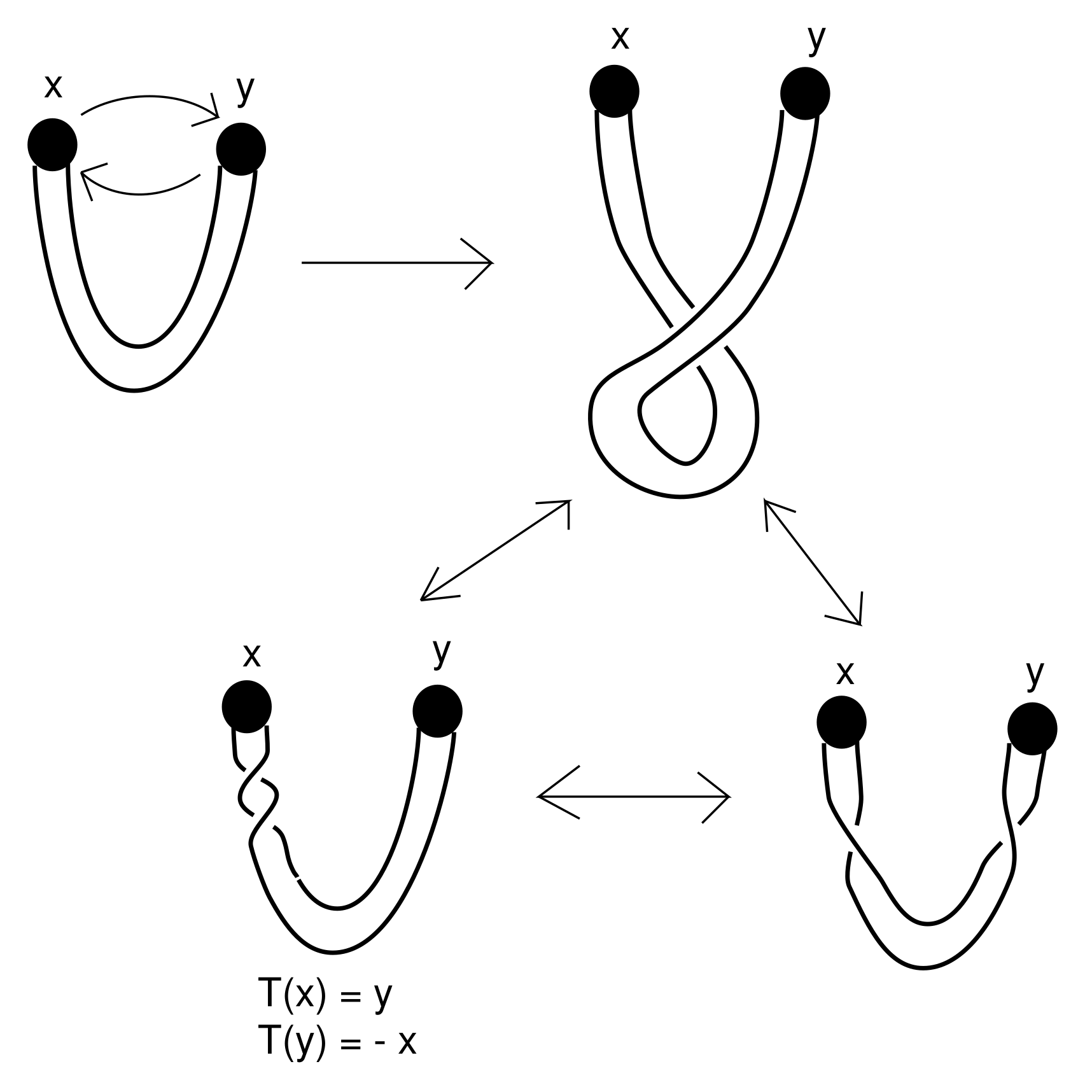
Distinction and processes arising from distinction are at the base of the described world. Distinctions are elemental bits of awareness. The world is composed not of things but processes and observations. It is the purpose of this paper to explore, from this perspective, a source of algebraic structures that have been important for the development of both mathematics and physics. We will discuss how basic Clifford algebra comes from very elementary processes such as an alternation of $\cdots +-+-+-\cdots$ and the fact that one can think of $\sqrt{-1}$ itself as a temporal iterant, a product of an $ϵ$ and an $\eta$ where the $ϵ$ is the $\cdots -+-+-+\cdots$ and the $\eta$ is a time shift operator. Clifford algebra is at the base of this mathematical world, and the fermions are composed of these things.

View Figure 1. The discrete process $\cdots -+-+-+\cdots$ can be seen as an iteration of $[+1,-1]$ or as an iteration of $[-1,+1].$ Along with the structure of ordered pairs $[a,b]$ and their component-wise addition and multiplication, we shall introduce a time-shifting operator $\eta$ so that

$$\eta [+1,-1]\eta =[-1,+1].$$

Figure 1. Iterants from discrete process.

Then, letting $i=[+1,-1]\eta ,$ we have

$$i^2=[+1,-1]\eta [+1,-1]\eta =[+1,-1][-1,+1]=[-1,-1]=-1.$$

Iterants formalize the intuition that i is a ± oscillation that interacts with itself through a delay of one time-step.

Section 2 is a discussion of the discrete Schrödinger equation and its relationship with iterants and with the complex numbers. We see how a discrete variant of the diffusion equation gives rise at once to both the complex numbers (as a summary of the iterant behaviour of this discretization of diffusion) and the Schrödinger equation as we know it. The section serves as an introduction to the key ideas in the rest of the paper. Section 3 and Section 4 are an introduction to the algebra of iterants and its relation with the square root of minus one. Section 4 shows how iterants produce $2\times 2$ matrix algebra and the split quaternions. Section 5 studies iterants of arbitrary period. We generalize the iterant construction to arbitrary finite groups $G.$ We show that by rearranging the multiplication table of the group so that the identity element appears on the diagonal, we get a set of permutation matrices representing the group faithfully as $n\times n$ matrices. Section 6 discusses the relationship of iterants with the Artin braid group. Each element of the braid group has an associated permutation. We generalize iterants so that the group acting on the vector part of the iterant is the Artin braid group. This leads to relationships with framed braids and we end the section with a description of a braided iterant formulation of the particle interaction model of Sundance Bilson-Thompson [16]. Section 7 is about Majorana Fermion operators and their associated anyonic braiding. This section is key for this paper in relation to the later sections on the Majorana Dirac equation, as we show in the later sections that the Clifford algebras of Majorana operators are fundamental for the structure of solutions to the Majorana-Dirac equation. It is a main point of this paper to make this connection in the full context of iterants. The connection between solutions of the Majorana-Dirac equation and Majorana operators will be the subject of our further research.

Section 8 gives an iterant interpretation of the $su\left(3\right)$ Lie algebra for the Standard Model. Section 9 discusses the Dirac equation and how the nilpotent and the Majorana operators work in this context. This section provides a link between our work, the work of Peter Rowlands [17] and with our joint work [1]. We end this section with an expression in split quaternions for the the Majorana Dirac equation in one dimension of time and three dimensions of space. The Majorana Dirac equation can be written as follows:

$$(\partial /\partial t+\widehat{\eta }\eta \partial /\partial x+ϵ\partial /\partial y+\widehat{ϵ}\eta \partial /\partial z-\widehat{ϵ}\widehat{\eta }\eta m)\psi =0$$

where $\eta$ and $ϵ$ are the simplest generators of iterant algebra with ${\eta }^2={ϵ}^2=1$ and $\eta ϵ+ϵ\eta =0,$ and $\widehat{ϵ},\widehat{\eta }$ make a commuting copy of this algebra. Combining the simplest Clifford algebra with itself is the underlying structure of Majorana Fermions, forming indeed the underlying structure of all Fermions. The Majorana-Dirac equation is expressed entirely with real matrices so that it can have solutions over the real numbers. It was Majorana’s conjecture that such solutions would correspond to particles that were their own anti-particles. Section 10 and Section 11 go on to study the original Majorana-Dirac equation and variations of involving the algebraic approach in this paper. We show how the nilpotent method described in Section 9 gives rise to solutions to this equation, hence to fundamental structures related to Majorana Fermions. This part of the paper reviews our work in [1] and sets the stage for future work.

2. Iterants and the Schrödinger Equation

We begin with the Diffusion Equation

$$\partial \psi /\partial t=\tau {\partial }^2\psi /\partial x^2.$$

We reformulate this equation as a difference equation in space and time. In writing it as a difference equation, I shall use $dt$ for a finite increment in time and $dx$ for a finite increment in space.

$$({\psi }_{t+dt}-{\psi }_t)/dt=\tau ({\psi }_t(x-dx)-2{\psi }_t\left(x\right)+{\psi }_t(x+dx))/{\left(dx\right)}^2.$$

This is equivalent to

$$({\psi }_{t+dt}-{\psi }_t)=\frac{dt}{{\left(dx\right)}^2}\tau ({\psi }_t(x-dx)-2{\psi }_t\left(x\right)+{\psi }_t(x+dx)),$$

or to

$$({\psi }_{t+dt}-{\psi }_t)=\kappa ({\psi }_t(x-dx)-2{\psi }_t\left(x\right)+{\psi }_t(x+dx)),$$

where $\kappa =\frac{dt}{{\left(dx\right)}^2}\tau ,$ since for the continuum limit to exist we need to assume that $\frac{dt}{{\left(dx\right)}^2}$ is constant as $dt$ and $dx$ go to zero. We shall use $dt=1$ for convenience.

Then the above equation becomes

$${\psi }_{t+1}-{\psi }_t=\kappa ({\psi }_t(x-dx)-2{\psi }_t\left(x\right)+{\psi }_t(x+dx)).$$

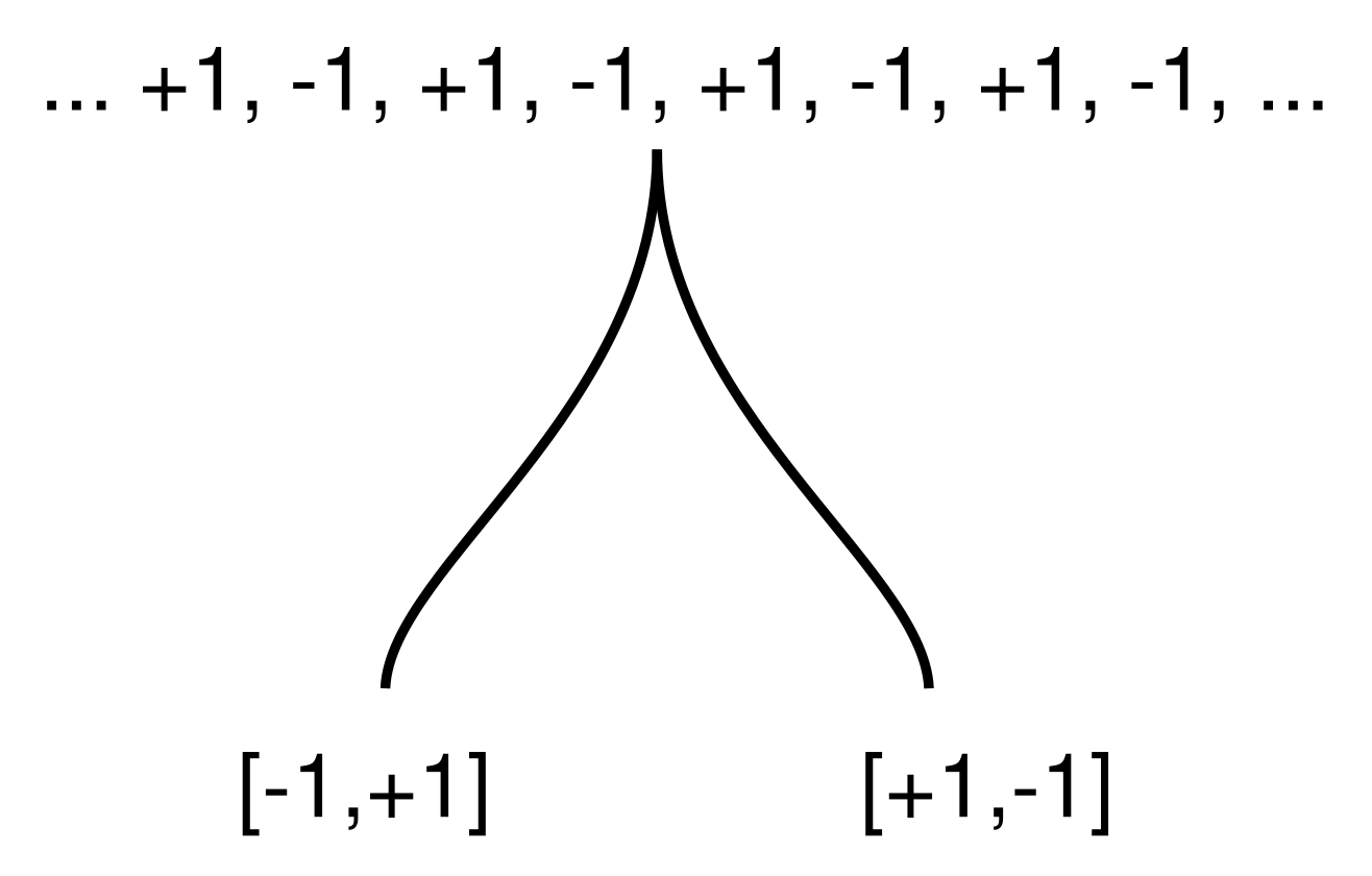
Consider the possibility of putting a “plus or minus” ambiguity into this equation, like so:

$$\partial \psi /\partial t=\pm \kappa {\partial }^2\psi /\partial x^2.$$

The ± coefficient should be lawful not random, for then we can follow an algebraic formulation of the process behind the equation. We shall take ± to mean the alternating sequence

$$\pm =\cdots +-+-+-+-\cdots$$

and time will be discrete. Then the new equation will become a difference equation in space and time

$${\psi }_{t+1}-{\psi }_t={(-1)}^t\kappa ({\psi }_t(x-dx)-2{\psi }_t\left(x\right)+{\psi }_t(x+dx)).$$

We must consider the continuum limit. But in that limit there is no direct meaning for the parity of the number of time steps

$${(-1)}^t.$$

In the discrete model the wave function $\psi$ divides into parts with even time index ${\psi }_e$ and parts with odd time index ${\psi }_o.$ So we can write (thinking of these as the corresponding discrete equations or as the continuum limits).

$${\partial }_t{\psi }_e=\kappa {\partial }_x^2{\psi }_o$$

$${\partial }_t{\psi }_o=-\kappa {\partial }_x^2{\psi }_e.$$

We take the limit of ${\psi }_e$ and ${\psi }_o$ separately.

Then one can interpret the $\{\pm \}$ as the complex number $i.$ Recall that the complex number i has the property that $i^2=-1$ so that

$$i(A+iB)=iA-B$$

when A and B are real numbers,

$$i=-1/i,$$

and so if $i=1$ then $i=-1,$ and if $i=-1$ then $i=1.$ So i can be interpreted as oscillating between $+1$ and $-1,$ and so we shall regard i as a definition of $\pm 1.$

$$i=\pm 1.$$

In fact, when we multiply $ii=(\pm 1)(\pm 1),$ we get $-1$ because (using this temporal interpretation) i takes a duration to oscillate and when the second term multiplies the first term, they are shifted by one step, and so we get either $(+1)(-1)=-1$ or $(-1)(+1)=-1.$ We formalize this point of view later in the paper.

Now $i=\pm 1$ behaves according to these rules, and we can write

$$\psi ={\psi }_e+i{\psi }_o$$

so that

$$i{\partial }_t\psi =i{\partial }_t({\psi }_e+i{\psi }_o)=i{\partial }_t{\psi }_e-{\partial }_t{\psi }_o$$

$$=i\kappa {\partial }_x^2{\psi }_o+\kappa {\partial }_x^2{\psi }_e=\kappa {\partial }_x^2({\psi }_e+i{\psi }_o)$$

$$=\kappa {\partial }_x^2\psi .$$

Thus

$$i\partial \psi /\partial t=\kappa {\partial }^2\psi /\partial x^2.$$

We have deduced the complex form of the Schrödinger equation as the limit of these discrete systems. In these systems there is a mutual dependency where the temporal variation of ${\psi }_e$ is mediated by the spatial variation of ${\psi }_o$ and the temporal variation of ${\psi }_o$ is mediated by the spatial variation of ${\psi }_e.$ We arrive at the Schrödinger equation in the context of $i=\pm$ as an iterant.

$${\partial }_t{\psi }_e=\kappa {\partial }_x^2{\psi }_o$$

$${\partial }_t{\psi }_o=-\kappa {\partial }_x^2{\psi }_e.$$

$$\psi ={\psi }_e+i{\psi }_o$$

$$i\partial \psi /\partial t=\kappa {\partial }^2\psi /\partial x^2.$$

Remark 1.

The discrete recursion, just discussed, can be implemented to approximate solutions to the Schrödinger equation. A further study of this recursion is intended. This way of thinking about the Schrödinger equation shows that it is intimately connected with a generalization of the discrete diffusion process with a parity oscillation that becomes i in the limit. The temporal interpretation of i indicated here will be given an algebraic context in the body of this paper.

3. Iterants and Idempotents

In this section we give a general context and formalization for the idea that the square root of negative unity can be regarded as an oscillation between $+1$ and $-1$ that is phase shifted with respect to itself via a time-step in the course of interacting with itself. We have used this idea in the previous section to motivate a discrete model of the Schrödinger equation. Here we will take an ordered pair $[1,-1]$ to represent the oscillation and a permutation operator $\eta$ to represent the time-step. The permutation operator will have order two and the property that $\eta [a,b]\eta =[b,a],$ effecting the phase shift of the oscillation $[-1,+1]$ to $[+1,-1].$ Then we can define $i=[-1,+1]\eta$ so that

$$i^2=[-1,+1]\eta [-1,+1]\eta =[-1,+1][+1,-1]=[-1,-1]=1.$$

The details of this construction are given below. The general form of the construction involves vectors and permutations. We will use Greek letters for permuation operators. They are not to be confused with any Greek letters in the previous section.

An iterant is a sum of elements of the form

$$[a_1,a_2,...,a_n]\sigma$$

where $[a_1,a_2,...,a_n]$ is a vector of scalars (real or complex numbers in most cases) and $\sigma$ is an element of the permutation group on n letters. The vectors are sums of elementary vectors of the form

$$[0,0,...0,1,0,...,0]\sigma =e_i\sigma$$

where the 1 is in the i-th place. The elements $e_i$ are the basic idempotents that generate the iterants with the help of the permutations.

If $a=[a_1,a_2,...,a_n]$, then we let $a^{\sigma }$ denote the vector with its elements permuted by the action of $\sigma .$

If a and b are vectors then $ab$ denotes the vector where ${\left(ab\right)}_i=a_i{b}_i,$ and $a+b$ denotes the vector where ${(a+b)}_i=a_i+b_i.$ Note that we define the usual sum of vectors and also the product of vectors as term-by-term combinations. Thus, for example,

$$[a,b,c]+[d,e,f]=[a+d,b+e,c+f]$$

and

$$[a,b,c][d,e,f]=[ad,be,cf].$$

Then, with vectors combined as above and the usual product (composition) of the permutations, we define products and sums of iterants as shown below.

$$\left(a\sigma \right)\left(b\tau \right)=\left(a{b}^{\sigma }\right)\sigma \tau ,$$

$$\left(ka\right)\sigma =k\left(a\sigma \right)$$

for a scalar k, and

$$(a+b)\sigma =a\sigma +b\sigma .$$

Iterant algebra is generated by the elements

$$e_i\sigma$$

where $e_i$ is a vector with a 1 in the i-th place and zeros elsewhere, and $\sigma$ is an abritrary element of the symmetric group $S_n.$ We have, by definition, that

$$e_i\sigma =\sigma e_j$$

where $\sigma \left(j\right)=i.$ In this way, multiplication of iterants is defined in terms of the action of the symmetric group on the vectors. For example, if $\sigma \in S_3$ is the cyclic permutation such that $\sigma \left(1\right)=2,\sigma \left(2\right)=3,\sigma \left(3\right)=1,$ then $e_2\sigma =\sigma e_1$ since $\sigma \left(1\right)=2.$ Similarly, $[c,b,a]\sigma =\sigma [a,b,c]$ for the cyclic permutation $\sigma$ in this paragraph.

By themselves, the elements $e_i$ are idempotent ($e_i^2=1$ for each i)and we have

$$1=e_1+\cdots e_n.$$

The iterant algebra is generated by these combinations of idempotents and permutations.

For example, if $\eta$ is the order two permutation of two elements, then ${[a,b]}^{\eta }=\eta [a,b]\eta =[b,a].$ Define the “shift" operator $\eta$ on iterants by the equation

$$\eta [a,b]=[b,a]\eta$$

with ${\eta }^2=1.$ Think of $\eta$ as a delay operator, since it shifts the waveform

$$\cdots ababab\cdots$$

by one internal time step. We can define

$$i=[-1,1]\eta$$

and then

$$i^2=[-1,1]\eta [-1,1]\eta =[-1,1]{[-1,1]}^{\eta }{\eta }^2=[-1,1][1,-1]=[-1,-1]=-1.$$

Complex numbers emerge from iterants. Interpret $[-1,1]$ as an oscillation between $-1$ and $+1$ and $\eta$ as a temporal shift operator. Then $i=[-1,1]\eta$ is time sensitive and its self-interaction equals minus one. Iterants are a formalization of elementary discrete processes. Let $ϵ=[-1,1].$ Then $i=ϵ\eta .$

We can write $a=[1,0],b=[0,1]$ and $A=a\eta ,B=b\eta$ where $\eta$ denotes the transposition so that $[x,y]\eta =\eta [y,x]$ and ${\eta }^2=1.$ Then we have

$$a^2=a,b^2=b,ab=0,a+b=1,A^2=0=B^2,AB=a,BA=b.$$

This is the mixed idempotent and permutation algebra for $n=2.$ Then we have

$$i=B-A$$

as we can see by

$$ii=(B-A)(B-A)=AA-AB-BA+BB=-a-b=-1.$$

This is the beginning of the relationships between idempotents, iterants and Clifford algebras.

We construct an elementary Clifford algebra via

$$ϵ=[-1,1]=b-a$$

and

$$\eta .$$

Then we have

$${ϵ}^2={\eta }^2=1$$

and

$$ϵ\eta +\eta ϵ=0.$$

Note also that the non-commuting of $ϵ$ and $\eta$ is directly related to the interaction of the idempotents and the permutations.

$$ϵ\eta =[-1,1]\eta =\eta [1,-1]=-\eta [-1,1]=-\eta ϵ.$$

4. Iterants, Discrete Processes and Matrix Algebra

In this section we relate iterants to matrix algebra. An elementary iterant is a periodic time series

$$\cdots abababababab\cdots .$$

The elements of the time series can be any mathematically well-defined objects. We regard ordered pairs $[a,b]$ and $[b,a]$ as abbreviations for the time series or as two points of view about the series (a first or b first). Call $[a,b]$ an iterant. One has the collection of transformations of the form $T[a,b]=[ka,k^{-1}b]$ leaving the product $ab$ invariant. This tiny model contains the seeds of special relativity, and the iterants contain the seeds of matrix algebra. See [4,5,18,19,20,21,22,23,24,25].

Define products and sums of iterants as follows

$$[a,b][c,d]=[ac,bd]$$

and

$$[a,b]+[c,d]=[a+c,b+d].$$

These operations are natural with respect to the structural juxtaposition of iterants:

$$...abababababab...$$

$$...cdcdcdcdcdcd...$$

Structures combine at the points where they correspond. Time series combine at the times where they correspond

If • denotes any form of binary compositon for the elements (a,b,...) of iterants, then we extend • to the iterants themselves by the definition $[a,b]•[c,d]=[a•c,b•d]$.

We now show how the iterant algebra is related to matrix algebra. In order to keep track of this patterning, lets write

$$[a,b]+[c,d]\eta =\left(\begin{array}{cc}a& c\\ d& b\end{array}\right)$$

where

$$[x,y]=\left(\begin{array}{cc}x& 0\\ 0& y\end{array}\right)$$

and

$$\eta =\left(\begin{array}{cc}0& 1\\ 1& 0\end{array}\right)$$

Recall the definition of matrix multiplication.

$$\left(\begin{array}{cc}a& c\\ d& b\end{array}\right)\left(\begin{array}{cc}e& g\\ h& f\end{array}\right)=\left(\begin{array}{cc}ae+ch& ag+cf\\ de+bh& dg+bf\end{array}\right)$$

Matrix multiplication is isomorphic with iterant multiplication.

$$\left(\right[a,b]+[c,d\left]\eta \right)\left(\right[e,f]+[g,h\left]\eta \right)=$$

$$[a,b][e,f]+[c,d]\eta [g,h]\eta +[a,b][g,h]\eta +[c,d]\eta [e,f]=$$

$$[ae,bf]+[c,d][h,g]+\left(\right[ag,bh]+[c,d\left]\right[f,e\left]\right)\eta =$$

$$[ae,bf]+[ch,dg]+\left(\right[ag,bh]+[cf,de\left]\right)\eta =$$

$$[ae+ch,dg+bf]+[ag+cf,de+bh]\eta$$

Notation. We have the shift operation $\eta [x,y]\eta =[y,x]$ which we shall denote by an overbar as shown below

$$\overline{[x,y]}=[y,x].$$

Ordinary matrix multiplication can be written in a concise form using the following rules:

$$\eta \eta =1$$

$$\eta Q=\overline{Q}\eta$$

where Q is any two element iterant. Note the correspondence

$$\left(\begin{array}{cc}a& b\\ c& d\end{array}\right)=\left(\begin{array}{cc}a& 0\\ 0& d\end{array}\right)\left(\begin{array}{cc}1& 0\\ 0& 1\end{array}\right)+\left(\begin{array}{cc}b& 0\\ 0& c\end{array}\right)\left(\begin{array}{cc}0& 1\\ 1& 0\end{array}\right)=[a,d]1+[b,c]\eta .$$

This means that $[a,d]$ corresponds to a diagonal matrix.

$$[a,d]=\left(\begin{array}{cc}a& 0\\ 0& d\end{array}\right),$$

$\eta$ corresponds to the anti-diagonal permutation matrix.

$$\eta =\left(\begin{array}{cc}0& 1\\ 1& 0\end{array}\right),$$

and $[b,c]\eta$ corresponds to the product of a diagonal matrix and the permutation matrix.

$$[b,c]\eta =\left(\begin{array}{cc}b& 0\\ 0& c\end{array}\right)\left(\begin{array}{cc}0& 1\\ 1& 0\end{array}\right)=\left(\begin{array}{cc}0& b\\ c& 0\end{array}\right).$$

Note also that

$$\eta [c,b]=\left(\begin{array}{cc}0& 1\\ 1& 0\end{array}\right)\left(\begin{array}{cc}c& 0\\ 0& b\end{array}\right)=\left(\begin{array}{cc}0& b\\ c& 0\end{array}\right).$$

This is the matrix interpretation of the equation

$$[b,c]\eta =\eta [c,b].$$

A two by two matrix is combinatorially the union of the identity pattern (the diagonal) and the interchange pattern (the antidiagonal). These correspond to the operators 1 and $\eta$ for iterants.

$$\left(\begin{array}{cc}*& @\\ @& *\end{array}\right)$$

In the case of complex numbers we represent

$$\left(\begin{array}{cc}a& -b\\ b& a\end{array}\right)=[a,a]+[-b,b]\eta =a1+b[-1,1]\eta =a+bi.$$

The square root of minus one takes the form of the matrix

$$i=ϵ\eta =[-1,1]\eta =\left(\begin{array}{cc}0& -1\\ 1& 0\end{array}\right).$$

If we identify the ordered pair $(a,b)$ with $a+ib,$ then this means taking the identification

$$(a,b)=\left(\begin{array}{cc}a& -b\\ b& a\end{array}\right).$$

$$i(a,b)=\left(\begin{array}{cc}0& -1\\ 1& 0\end{array}\right)\left(\begin{array}{cc}a& -b\\ b& a\end{array}\right)=\left(\begin{array}{cc}-b& -a\\ a& -b\end{array}\right)=b+ia=(-b,a).$$

In iterant terms we have

$$i[a,b]=ϵ\eta [a,b]=[-1,1][b,a]\eta =[-b,a]\eta ,$$

and this corresponds to the matrix equation

$$i[a,b]=\left(\begin{array}{cc}0& -1\\ 1& 0\end{array}\right)\left(\begin{array}{cc}a& 0\\ 0& b\end{array}\right)=\left(\begin{array}{cc}0& -b\\ a& 0\end{array}\right)=[-b,a]\eta .$$

More generally, we see that

$$(A+B\eta )(C+D\eta )=(AC+B\overline{D})+(AD+B\overline{C})\eta$$

writing the $2\times 2$ matrix algebra as a system of hypercomplex numbers. Note that

$$(A+B\eta )(\overline{A}-B\eta )=A\overline{A}-B\overline{B}$$

The formula on the right equals the determinant of the matrix. Thus we define the conjugate of $Z=A+B\eta$ by the formula

$$\overline{Z}=\overline{A+B\eta }=\overline{A}-B\eta ,$$

and we have the formula

$$D\left(Z\right)=Z\overline{Z}$$

for the determinant $D\left(Z\right)$ where

$$Z=A+B\eta =\left(\begin{array}{cc}a& c\\ d& b\end{array}\right)$$

where $A=[a,b]$ and $B=[c,d].$ Note that

$$A\overline{A}=[ab,ba]=ab1=ab,$$

so that

$$D\left(Z\right)=ab-cd.$$

Note also that we assume that $a,b,c,d$ are in a commutative base ring.

Note also that for Z as above,

$$\overline{Z}=\overline{A}-B\eta =\left(\begin{array}{cc}b& -c\\ -d& a\end{array}\right).$$

This is the classical adjoint of the matrix $Z.$

We leave it to the reader to check that for matrix iterants Z and $W,$

$$Z\overline{Z}=\overline{Z}Z$$

and that

$$\overline{ZW}=\overline{WZ}$$

and

$$\overline{Z+W}=\overline{Z}+\overline{W}.$$

Note also that

$$\overline{\eta }=-\eta ,$$

whence

$$\overline{B\eta }=-B\eta =-\eta \overline{B}=\overline{\eta }\overline{B}.$$

We can prove that

$$D\left(ZW\right)=D\left(Z\right)D\left(W\right)$$

as follows

$$D\left(ZW\right)=ZW\overline{ZW}=ZW\overline{W}\overline{Z}=Z\overline{Z}W\overline{W}=D\left(Z\right)D\left(W\right).$$

That $W\overline{W}$ is in the commutative base ring allows us to remove it from in between the appearance of Z and $\overline{Z}.$ Iterants as $2\times 2$ matrices form a direct non-commutative generalization of the complex numbers.

The split quaternions are the system

$$\{\pm 1,\pm ϵ,\pm \eta ,\pm i\}.$$

The quaternions arise directly from the split quaternions once we construct an extra square root of minus one that commutes with them. Call this extra root of minus one $\sqrt{-1}$. Then the quaternions are generated by

$$I=\sqrt{-1}ϵ,J=ϵ\eta ,K=\sqrt{-1}\eta$$

with

$$I^2=J^2=K^2=IJK=-1.$$

In the next section we give a number of other ways to construct the quaternions, and we show how the iterant point of view is related to matrix representations of the quaternions such as matrices over the complex numbers in $SU\left(2\right).$

5. Iterants of Arbirtarily High Period

As a next example, consider a waveform of period three.

$$\cdots abcabcabcabcabcabc\cdots$$

Here we see three viewpoints (depending upon whether one starts at a, b or c).

$$[a,b,c],[b,c,a],[c,a,b].$$

The appropriate shift operator is given by the formula

$$[x,y,z]S=S[z,x,y].$$

Thus, with $T=S^2,$

$$[x,y,z]T=T[y,z,x]$$

and $S^3=1.$ With this we obtain a closed algebra of iterants whose general element is of the form

$$[a,b,c]+[d,e,f]S+[g,h,k]S^2.$$

in this formalism $a,b,c,d,e,f,g,h,k$ are real or complex numbers. The algebra is denoted $\mathbb{V}ec{t}_3\left(\mathbb{R}\right)$ with the scalars in a commutative ring with unit $\mathbb{F}.$ For matrices, $M_3\left(\mathbb{F}\right)$ is the $3\times 3$ matrix algebra over $\mathbb{F}.$

Lemma 1.

Iterant algebra $\mathbb{V}ec{t}_3\left(\mathbb{F}\right)$ is isomorphic to the $3\times 3$ matrix algebra $M_3(\left(\mathbb{F}\right).$

Proof. 

Map 1 to the matrix

$$\left(\begin{array}{ccc}1& 0& 0\\ 0& 1& 0\\ 0& 0& 1\end{array}\right).$$

Map S to the matrix

$$\left(\begin{array}{ccc}0& 1& 0\\ 0& 0& 1\\ 1& 0& 0\end{array}\right),$$

and map $S^2$ to the matrix

$$\left(\begin{array}{ccc}0& 0& 1\\ 1& 0& 0\\ 0& 1& 0\end{array}\right),$$

Map $[x,y,z]$ to the diagonal matrix

$$\left(\begin{array}{ccc}x& 0& 0\\ 0& y& 0\\ 0& 0& z\end{array}\right).$$

Then it follows that

$$[a,b,c]+[d,e,f]S+[g,h,k]S^2$$

maps to the matrix

$$\left(\begin{array}{ccc}a& d& g\\ h& b& e\\ f& k& c\end{array}\right),$$

preserving the algebra structure. It follows that $\mathbb{V}ec{t}_3\left(\mathbb{F}\right)$ is isomorphic to the full $3\times 3$ matrix algebra $M_3\left(\mathbb{F}\right).$ □

The pattern behind the $3\times 3$ matrices is held by the symbolic matrix

$$\left(\begin{array}{ccc}1& S& T\\ T& 1& S\\ S& T& 1\end{array}\right).$$

T occupies positions in the matrix corresponding to a permutation matrix. The letter S occupies the positions corresponding to its permutation matrix. The 1’s occupy the diagonal for the an identity matrix. In this case the matrices form a permutation representation of the cyclic group of order 3, $C_3=\{1,S,S^2\}.$

It should be clear to the reader that this construction generalizes directly for iterants of any period and hence for a set of operators forming a cyclic group of any order. In fact we can generalize further to any finite group $G.$ See [13] for more information about these generalizations.

• In this example we consider the group $G=C_2\times C_2,$ often called the “Klein 4-Group." We take $G=\{1,A,B,C\}$ where $A^2=B^2=C^2=1,AB=BA=C.$ Thus G has the multiplication table, which is also its G-Table for $\mathbb{V}ec{t}_4(G,\mathbb{F}).$

  $$\left(\begin{array}{cccc}1& A& B& C\\ A& 1& C& B\\ B& C& 1& A\\ C& B& A& 1\end{array}\right).$$
  Thus we have the permutation matrices that I shall call $E,A,B,C$ whose entries are obtained from the matrix above by writing 1 for the places occupied by the corresponding letter and 0 for the other places. For example,

  $$A=\left(\begin{array}{cccc}0& 1& 0& 0\\ 1& 0& 0& 0\\ 0& 0& 0& 1\\ 0& 0& 1& 0\end{array}\right).$$
  The reader will verify that $A^2=B^2=C^2=1,AB=BA=C.$ Recall that $[x,y,z,w]$ is iterant notation for the diagonal matrix

  $$[x,y,z,w]=\left(\begin{array}{cccc}x& 0& 0& 1\\ 0& y& 1& 0\\ 0& 1& z& 0\\ 1& 0& 0& w\end{array}\right).$$
  Let

  $$\alpha =[1,-1,-1,1],\beta =[1,1,-1,-1],\gamma =[1,-1,1,-1].$$
  And let

  $$I=\alpha A,J=\beta B,K=\gamma C.$$
  Then we have

  $$I^2=J^2=K^2=IJK=-1,IJ=K,JI=-K.$$
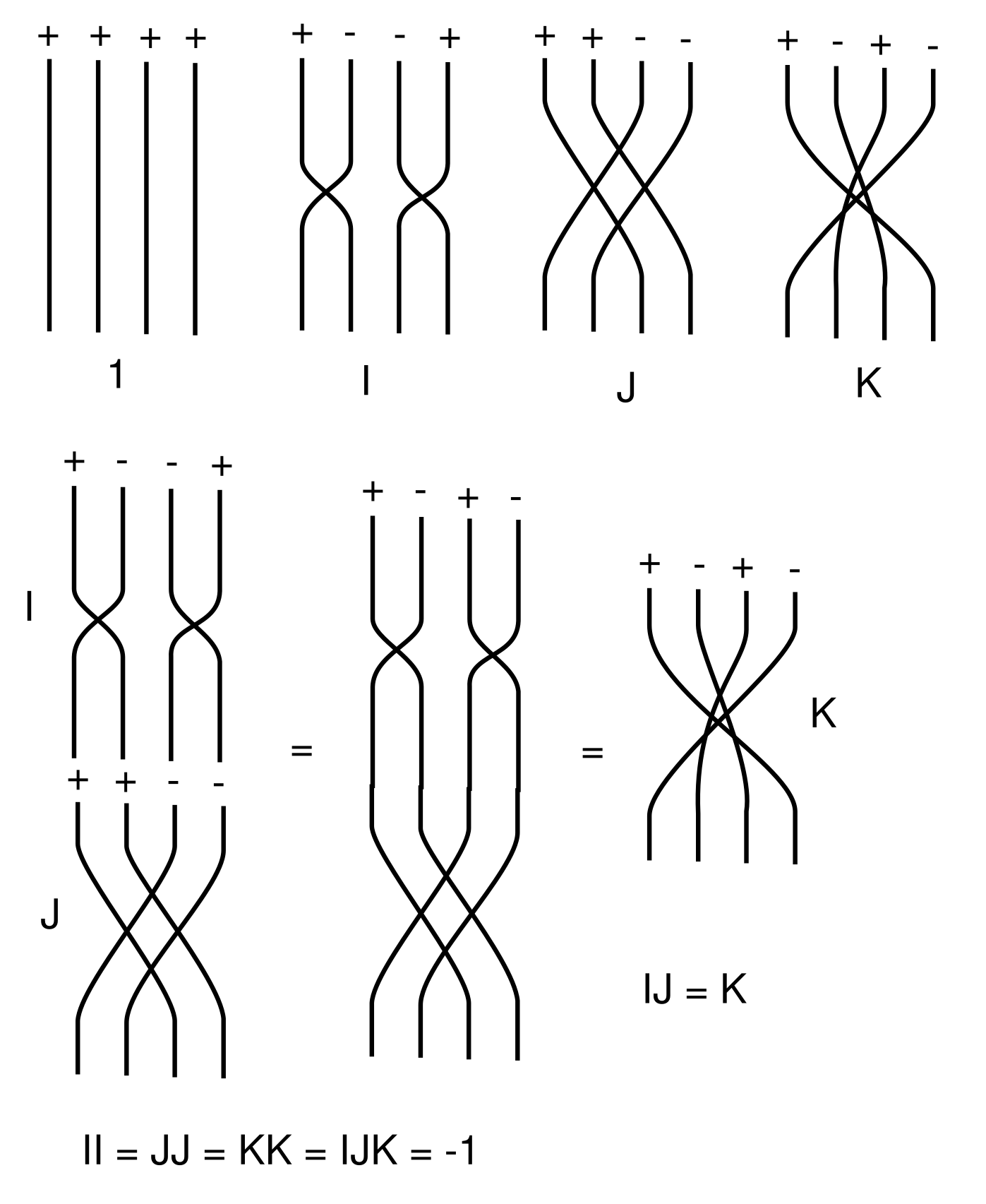
  The quaternions are iterants in relation to the Klein Four Group. Figure 2 illustrates these quaternion generators with string diagrams for the permutations. The reader can check that the permutations correspond to the permutation matrices constructed for the Klein Four Group.
  

  Figure 2. Quaternions from the Klein Four group.
• The set of matrices of the form $a1+bI+cJ+dK$ with $a^2+b^2+c^2+d^2=1$ is isomorphic to the group $SU\left(2\right).$ To see this, note that $SU\left(2\right)$ is the set of matrices with complex entries z and w with determinant 1 so that $z\overline{z}+w\overline{w}=1.$

  $$M=\left(\begin{array}{cc}z& w\\ -\overline{w}& \overline{z}\end{array}\right).$$
  Letting $z=a+bi$ and w = $c+di,$ we have -4.6cm0cm

  $$M=\left(\begin{array}{cc}a+bi& c+di\\ -c+di& a-bi\end{array}\right)=a\left(\begin{array}{cc}1& 0\\ 0& 1\end{array}\right)+b\left(\begin{array}{cc}i& 0\\ o& -i\end{array}\right)+c\left(\begin{array}{cc}0& 1\\ -1& 0\end{array}\right)+d\left(\begin{array}{cc}0& i\\ i& 0\end{array}\right).$$
  With a commutative $i=\sqrt{-1}$ we obtain

  $$I=\sqrt{-1}ϵ,J=ϵ\eta ,K=\sqrt{-1}\eta$$

  as described in the previous section. This construction shows how the structure of the quaternions comes directly from the non-commutative structure of period two iterants. In other, words, quaternions can be represented by $2\times 2$ matrices. This is the way it has been presented in standard language as in the group $SU\left(2\right).$
• Here $\iota =\sqrt{-1}.$ Let

  $$H=[a,b]+[c+d\iota ,c-d\iota ]\eta =\left(\begin{array}{cc}a& c+d\iota \\ c-d\iota & b\end{array}\right).$$

  represents a Hermitian $2\times 2$ matrix and hence an observable for quantum processes mediated by $SU\left(2\right).$ Hermitian matrices have real eigenvalues.
  Take $a=T+X,b=T-X,c=Y,d=Z,$ then we obtain an iterant representation for a point in Minkowski spacetime.

  $$H=[T+X,T-X]+[Y+Z\iota ,Y-Z\iota ]\eta =\left(\begin{array}{cc}T+X& Y+Z\iota \\ Y-Z\iota & T-X\end{array}\right).$$
  Note that we have the formula

  $$Det\left(H\right)=T^2-X^2-Y^2-Z^2.$$
  The eigenvalues of H are $T\pm \sqrt{X^2+Y^2+Z^2}.$ H can observe the time and the invariant spatial distance from the origin of the event $(T,X,Y,Z).$ Here quantum mechanics and special relativity are reconciled.
• Iterants generate Hamilton’s Quaternions. We express them algebraically as shown below.

  $$I=[+1,-1,-1,+1]s$$

  $$J=[+1,+1,-1,-1]l$$

  $$K=[+1,-1,+1,-1]t$$

  where

  $$s=\left(12\right)\left(34\right)$$

  $$l=\left(13\right)\left(24\right)$$

  $$t=\left(14\right)\left(23\right).$$
  The permutations are products of transpositions $\left(ij\right).$
  One can verify that

  $$I^2=J^2=K^2=IJK=-1.$$
  For example,

  $$I^2=[+1,-1,-1,+1]s[+1,-1,-1,+1]s$$

  $$=[+1,-1,-1,+1][-1,+1,+1,-1]ss$$

  $$=[-1,-1,-1,-1]$$

  $$=-1.$$

  and

  $$IJ=[+1,-1,-1,+1]s[+1,+1,-1,-1]l$$

  $$=[+1,-1,-1,+1][+1,+1,-1,-1]sl$$

  $$=[+1,-1,+1,-1]\left(12\right)\left(34\right)\left(13\right)\left(24\right)$$

  $$=[+1,-1,+1,-1]\left(14\right)\left(23\right)$$

  $$=[+1,-1,+1,-1]t.$$

  Remark 2. 

  We take an eigenform to mean a fixed point for a transformation in any mathematical domain. Transformations of a given domain do not always have fixed points in that domain. For example in a boolean logical domain the avaliable values are 0 and $1.$ If we take the transformation $T\left(x\right)=\sim x,$ then $T\left(0\right)=1$ and $T\left(1\right)=0$ so that there is no fixed point for $T.$ There is no boolean value J such that $\sim J=J.$ We can make extended logics that contain such values. Similarly, there is no fixed point for $G\left(x\right)=1+1/x$ in the rational numbers, since such a fixed point would equal an irrational number. Finally, in the real numbers there is no fixed point for the transformaton $R\left(x\right)=-1/x$ since such a fixed point would have square equal to minus one. If we have a domain D where every element of the domain corresponds to a mapping of the domain to itself, then one can define special transformations of the form $Gx=F\left(xx\right)$ for every F in $D.$ Then $GG=F\left(GG\right)$ and every F in D has a fixed point. This is the method of the lambda calculus of Church and Curry [4]. Constructions for fixed points that extend given domains is a way of thinking about the nature of our constructions in this paper. This theme is the subject of other work of the author [26]. Here i is an eigenform for $R\left(x\right)=-1/x.$ Indeed, each generating quaternion is an eigenform for the transformation $R\left(x\right)=-1/x.$ The richness of the quaternions comes from the closed algebra that arises with its infinity of eigenforms that satisfy the equation $U^2=-1:$$U=aI+bJ+cK$ where $a^2+b^2+c^2=1.$
• Clifford algebras $C_n$ generated by elements $\{e_1,e_2,\cdots ,e_n\}$ with $e_i^2=1$ and $e_i{e}_j=-e_j{e}_i$ when $i\ne j$ occur very often in both mathematics and physics. These algebras are often used as part of what is called geometric algebra [27]. It is worth noting that these algebras fit naturally into the iterants framework via their self-action. That is, if we take $C_n$ as a vector space over a field K, then it has basis consisting of all the ordered products of the form $e_{i_1}{e}_{i_2}\cdots e_{i_k}$ for $k=1,2,\cdots ,n$ and $i_1<i_2<\cdots <i_k.$ We can list the basis and obtain signed permutation matrices that represent the left action of the algebra on itself, just as we have done with the group representations in this section. For example, when n = 2 we have the basis list $(1,e_1,e_2,e_1{e}_2)$ and $e_1(1,e_1,e_2,e_1{e}_2)=(e_1,1,e_1{e}_2,e_2)$ while $e_2(1,e_1,e_2,e_1{e}_2)=(e_2,-e_1{e}_2,1,-e_2).$ Thus if $\sigma =\left(12\right)\left(34\right)$ and $\tau =\left(13\right)\left(24\right)$, then we can represent $e_1=[1,1,1,1]\sigma$ and $e_2=[1,-1,1,-1]\tau$ as iterants. In the case $n=2$ we have already given a simpler iterant representation of this algebra at the beginning of the paper, using $e_1=[-1,+1]$ and $e_2=\eta$ where $\eta$ denotes the transposition in $S_2.$ It is interesting how this representation appears doubled in the one we deduced from the multiplication table of the algebra. It is of interest to carry out corresponding calculations for higher values of $n.$

6. Iterants Associated with the Framed Braid Group

The Symmetric Group $S_n$ has presentation

$$S_n=(T_1,\cdots T_{n-1}|T_i^2=1,T_i{T}_{i+1}{T}_i=T_{i+1}{T}_i{T}_{i+1},T_i{T}_j=T_j{T}_i;|i-j|>1).$$

The Artin Braid Group $B_n$ has presentation

$$B_n=({\sigma }_1,\cdots {\sigma }_{n-1}|{\sigma }_i{\sigma }_{i+1}{\sigma }_i={\sigma }_{i+1}{\sigma }_i{\sigma }_{i+1},{\sigma }_i{\sigma }_j={\sigma }_j{\sigma }_i;|i-j|>1).$$

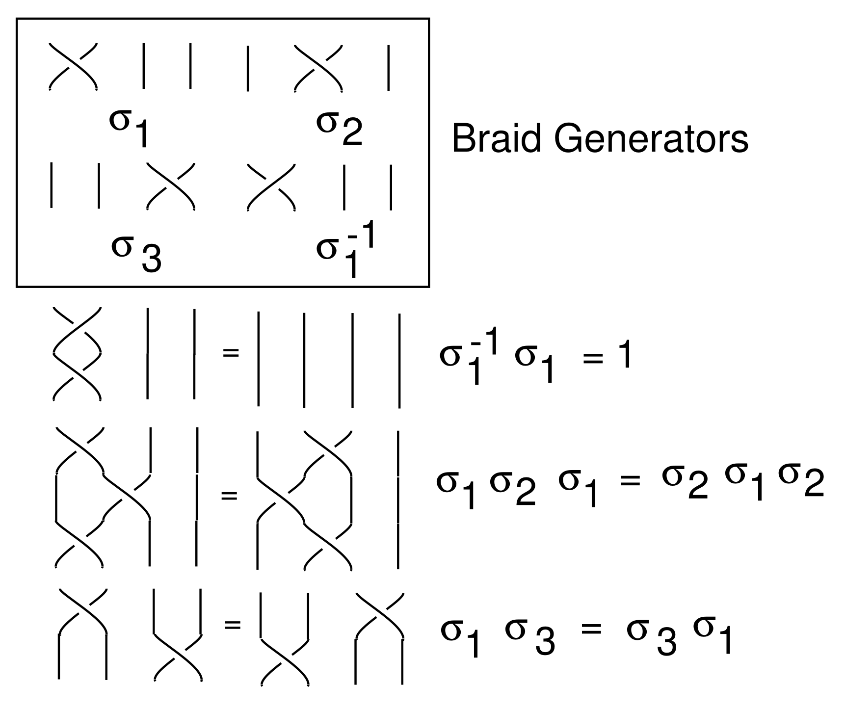
Thus there is a natural homomorphism from the Artin Braid Group to the Symmetric Group. In Figure 3 are shown the generators ${\sigma }_1,{\sigma }_2,{\sigma }_3$ of the 4-strand braid group with the topological relation ${\sigma }_1{\sigma }_2{\sigma }_1={\sigma }_2{\sigma }_1{\sigma }_2$ and the commuting relation ${\sigma }_1{\sigma }_3={\sigma }_3{\sigma }_1.$ The elementary braid generators ${\sigma }_i$ correspond to the interchange of the i-th strand iwith the $i+1$-th strand.

Figure 3. Braid Generators.

The homomorphism $\pi :B_n⟶S_n$ defined on generators by $\pi \left({\sigma }_i\right)=T_i.$ It is natural to generalize iterants to braided iterants by first generalizing the braid group to the framed braid group. In this generalization, we associate integers $t^a$ to the top of each braid strand. One can replace each braid strand by a ribbon and interpret $t^a$ as a $2\pi a$ twist in the ribbon. In Figure 4 it is shown how to multiply two framed braids. The braids A and B are given by the formulas

$$A=[t^a,t^b,t^c]{\sigma }_1{\sigma }_2{\sigma }_3,$$

$$B=[t^d,t^e,t^f]{\sigma }_2{\sigma }_3.$$

The framed braid group on three strands is denoted $F{B}_3.$ As the Figure 4 illustrates, there is the formula

$$v\sigma =\sigma v^{\pi \left(\sigma \right)}$$

where v is a vector of the form $v=[t^a,t^b,t^c]$ (for $n=3$) and $v^{\pi \left(\sigma \right)}$ is the result of permuting the vector by the permutation associated with the braid.

Figure 4. Framed Braids.

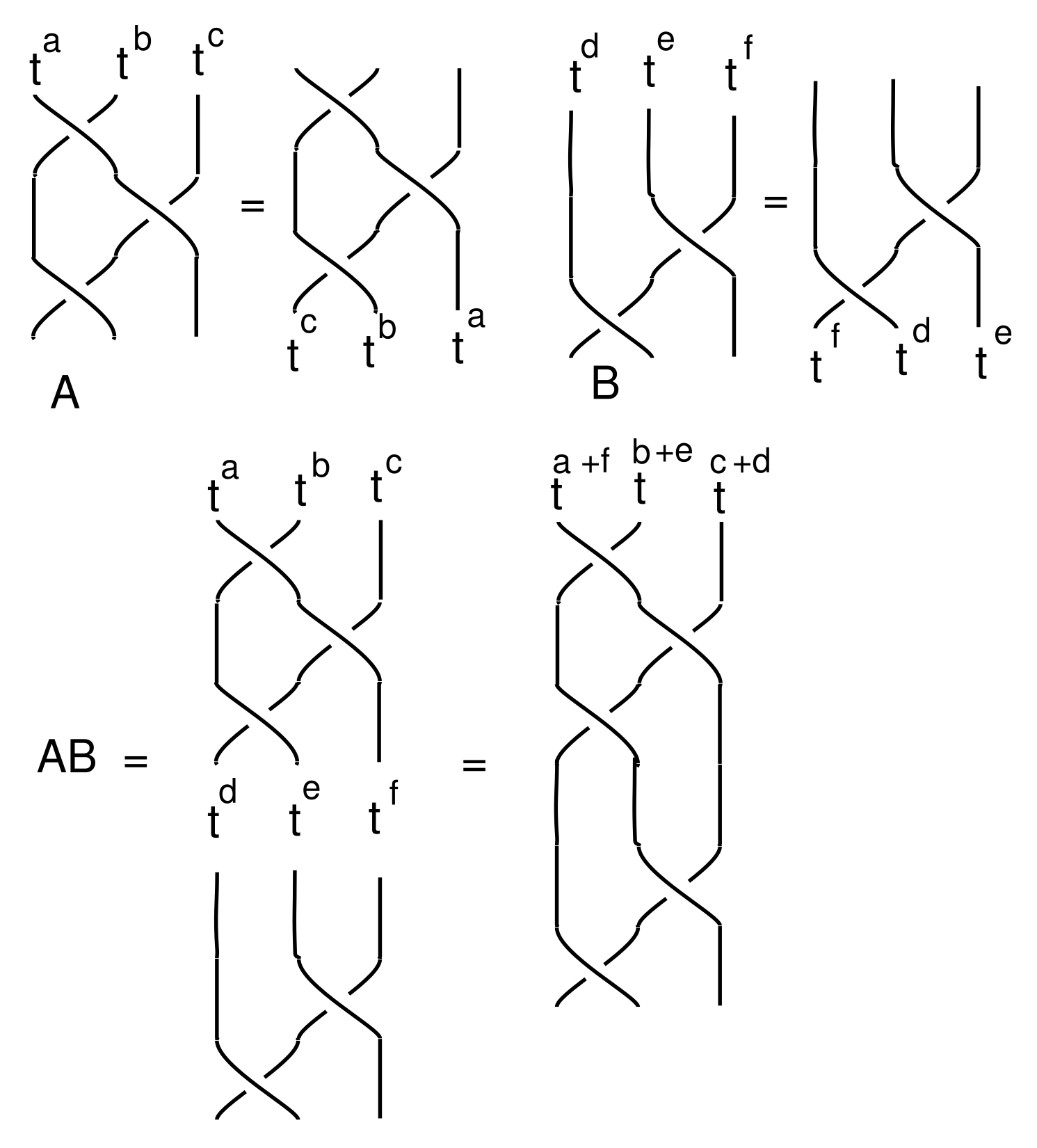
We can form an algebra $Alg\left[F{B}_n\right]$ by taking formal sums of framed braids of the form $\sum c_k{v}_k{g}_k$ where $c_k$ is a scalar, $v_k$ is a framing vector and $g_k$ is an element of the Artin Braid group $B_n.$ This algebra is a generalization of iterant algebra, based on the action of the Artin Braid Group. The representation $\pi :B_n⟶S_n$ induces a map of algebras $\widehat{\pi }:Alg\left[F{B}_n\right]⟶Alg\left[F{S}_n\right]$ where we recognize $Alg\left[F{S}_n\right]$ as exactly an iterant algebra based in the symmetric group $S_n.$

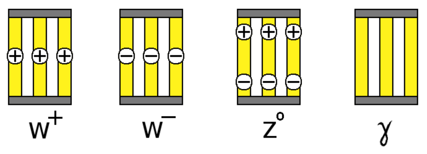
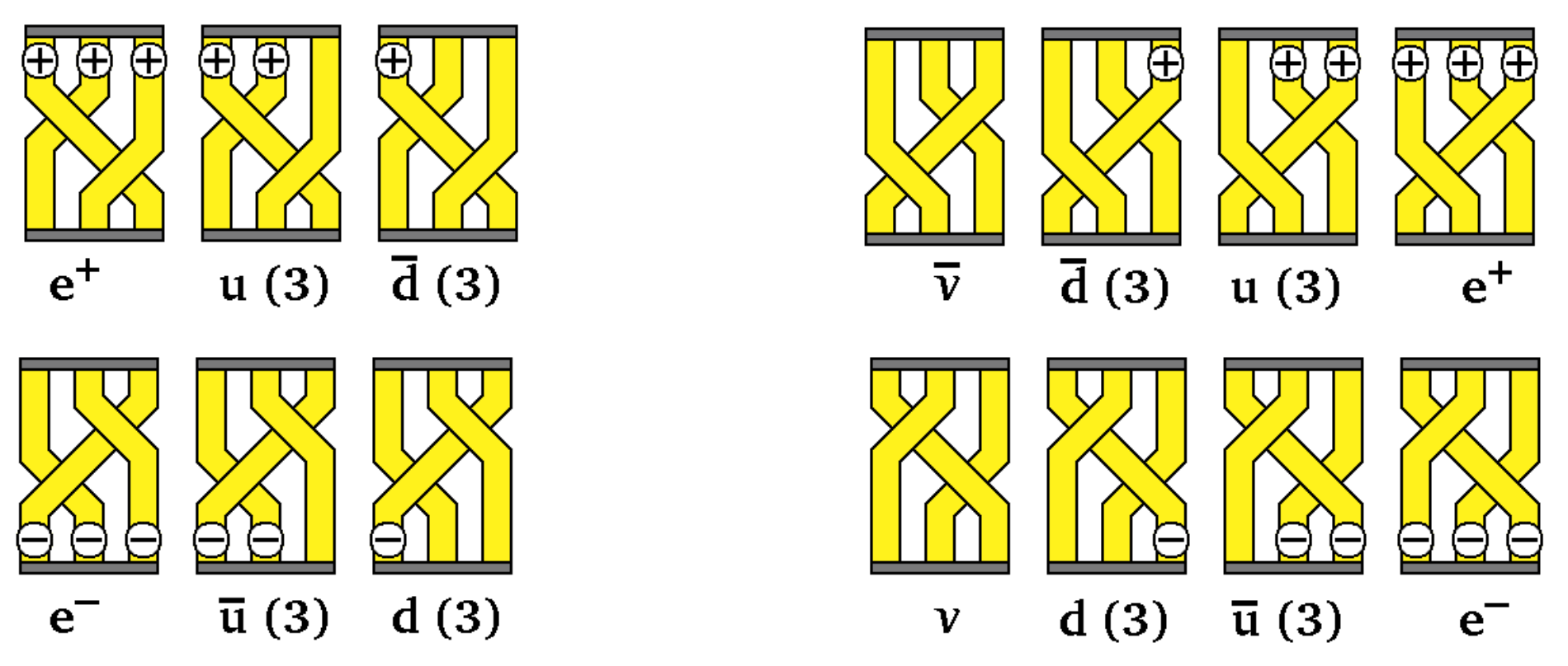
In [16] Fermions are represented as framed braids. See Figure 5. The positron and the electron are given by the framed braids

$$e^{+}=[t,t,t]{\sigma }_1{\sigma }_2^{-1},$$

and

$$e^{-}={\sigma }_2{\sigma }_1^{-1}[t^{-1},t^{-1},t^{-1}],$$

Figure 5. Sundance Bilson-Thompson Fermions.

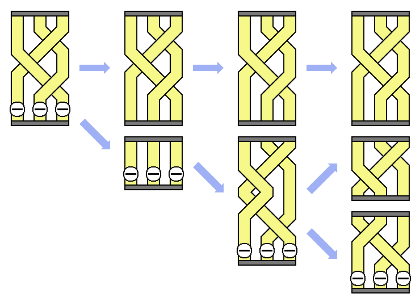
Here we use $[t^a,t^b,t^c]$ for the framing numbers $(a,b,c).$ Products of framed braids catalog particle interactions. The electron and the positron are algebraic inverses. In Figure 6 are bosons, including a photon $\gamma .$ Figure 7 illustrates the muon decay

$$\mu \to {\nu }_{\mu }+W_{-}\to {\nu }_{\mu }+\overline{{\nu }_e}+e^{-}.$$

Figure 6. Bosons.

Figure 7. Representation of $\mu \to {\nu }_{\mu }+W_{-}\to {\nu }_{\mu }+\overline{{\nu }_e}+e^{-}$.

The muon decay is a multiplicative identity in the braid algebra:

$$\mu ={\nu }_{\mu }{W}_{-}={\nu }_{\mu }\overline{{\nu }_e}{e}^{-}.$$

7. Fermions, Majorana Fermions and Anyonic Braiding

In this section we consider the algebras of Femions and Majorana fermions. The generators of this Clifford algebra represent fermions that are their own anti-particles. For a long time it has been conjectured that neutrinos may be Majorana fermions. More recently, it has been suggested that Majorana fermions may occur in collective electronic phenomena and in subtle correlations in nano-wires and in two dimensional anyonic physics [28,29,30,31].

In order to explain this association, we first give a short exposition of the algebra of fermion operators. In a standard collection of fermion operators $m_1,\cdots ,m_k$ one has that each $m_i$ is a linear operator on a Hilbert space with an adjoint operator $m_i^{†}$ (corresponding to the anti-particle for the particle created by $m_i$) and relations

$$m_i^2=0,$$

$$m_i{m}_i^{†}+m_i^{†}{m}_i=1,$$

$$m_i{m}_j+m_j{m}_i=0$$

when $i\ne j.$

There is another brand of Fermion algebra where we have generators $c_1,\cdots c_k$ and $c_i^2=1$ while $c_i{c}_j=-c_j{c}_i$ for all $i\ne j.$ These are the Majorana fermions. There is a algebraic translation between the fermion algebra and Majorana fermion algebra. Given two Majorana fermions a and b with $a^2=b^2=1$ and $ab=-ba,$ define

$$m=(a+ib)/2$$

and

$$m^{†}=(a-ib)/2.$$

It is then easy to see that $a^2=b^2=1$ and $ab=-ba$ imply that m and $m^{†}$ form a fermion in the sense that $m^2={\left(m^{†}\right)}^2=0$ and $m{m}^{†}+m^{†}m=1.$ Thus pairs of Majorana fermions can be construed as ordinary fermions. Conversely, if m is an ordinary fermion, then formal real and imaginary parts of m yield a mathematical pair of Majorana fermions. A chain of electrons in a nano-wire, conceived in this way can give rise to a chain of Majorana fermions with a non-localized pair corresponding to the distant ends of the chain. The non-local nature of this pair is promising for creating topologically protected qubits, and there is at this writing an experimental search for evidence for the existence of such end-effect Majorana fermions.

Remark 3.

It is common to refer to the Clifford algebra generated by a and b with $a^2=b^2=1$ and $ab=-ba$ as a pair of Majorana Fermions. The reference is to Majorana [30] who rewrote the Dirac equation so that it could be seen as a coupled system of equations over the real numbers. This Majorana-Dirac equation can have solutions that are their own anti-particles. This is reflected in the algebra where $a^{†}=a$ and $b^{†}=b.$ The Fermion operators that we construct from these Majorana operators $m=(a+ib)/2$ and $m^{†}=(a-ib)/2$ form a particle-antiparticle pair. It is of interest to see if the Majorana operators actually are related to Majorana’s original formalism. It is one of the main points of this paper that this is the case. See Sections 9 through 11 for more about this point. This paper and its predecessor [1] are a beginning for us in uncovering deeper relationships between Majorana operators as Clifford algebra and the properties of the Majorana-Dirac equation.

Here is an example that shows how topology is related to the Majorana Fermion operators. Let $x,y,z$ be three Majorana fermions. Let $A=yx,B=zy,C=xz.$ We have already seen that $A,B,C$ represent the quaternions. Now define

$${\sigma }_1=(1+A)/\sqrt{2},{\sigma }_2=(1+B)/\sqrt{2},{\sigma }_3=(1+C)/\sqrt{2}.$$

It is easy to see that ${\sigma }_i$ and ${\sigma }_j$ satisfy the braiding relation for any $i\ne j.$ For example, here is the verification for $i=1,j=2.$

$${\sigma }_1{\sigma }_2{\sigma }_1=(1/2\sqrt{2})(1+A)(1+B)(1+A)$$

$$=(1/2\sqrt{2})(1+A+B+AB)(1+A)$$

$$=(1/2\sqrt{2})(1+A+B+AB+A+A^2+BA+ABA)$$

$$=(1/2\sqrt{2})(1+A+B+AB+A-1-AB+B)$$

$$=(1/\sqrt{2})(A+B).$$

Similarly,

$${\sigma }_2{\sigma }_1{\sigma }_2=(1/2\sqrt{2})(1+B)(1+A)(1+B)$$

$$=(1/2\sqrt{2})(1+A+B+BA)(1+B)$$

$$=(1/2\sqrt{2})(1+A+B+BA+B+AB+B^2+BAB)$$

$$=(1/2\sqrt{2})(1+A+B+BA+B-BA-1+A)$$

$$=(1/\sqrt{2})(A+B).$$

Thus

$${\sigma }_1{\sigma }_2{\sigma }_1={\sigma }_2{\sigma }_1{\sigma }_2,$$

and so a natural braid group representation arises from the Majorana fermions. This braid group representation is significant for possible applications in topological quantum computing. For the purpose of this discussion, the braid group representation shows that the Clifford algebraic representation for knot sets is related to topology at more than one level. The relation $x^2=1$ for generators makes the individual sets, taken as products of generators, invariant under the Reidemeister moves (up to a global sign). But braiding invariance of certain linear combinations of sets is a relationship with knotting at a second level. This multiple relationship certainly deserves more thought. We will make one more remark here, and reserve further analysis for a subsequent paper.

The braiding operators act on the complex vector space spanned by the fermions $x,y,z.$

$$\sigma =\frac{1+yx}{\sqrt{2}},$$

$$T\left(p\right)=\sigma p{\sigma }^{-1}=\left(\frac{1+yx}{\sqrt{2}}\right)p\left(\frac{1-yx}{\sqrt{2}}\right),$$

It follows that $T\left(x\right)=y$ and $T\left(y\right)=-x.$ In Figure 8 where we show an interpretation for the braiding of two fermions. In the interpretation the two fermions are joined by a belt. On particle interchange, the belt is twisted by $2\pi .$ A twist of $2\pi$ corresponds to a phase change of $-1.$ See [32]. It may not be evident which particle should receive the phase change. Topology alone tells only the relative change of phase. The Clifford algebra makes a specific choice and so fixes the representation of the braiding.

Figure 8. Braiding Action on a Pair of Fermions.

8. Iterants and the Standard Model

Here we give an iterant interpretation for the Lie algebra of the special unitary group $SU\left(3\right).$ The Lie algebra $su\left(3\right)$ is generated by the following eight Gell Man Matrices [33].

$${\lambda }_1=\left(\begin{array}{ccc}0& 1& 0\\ 1& 0& 0\\ 0& 0& 0\end{array}\right),{\lambda }_2=\left(\begin{array}{ccc}0& -i& 0\\ i& 0& 0\\ 0& 0& 0\end{array}\right),{\lambda }_3=\left(\begin{array}{ccc}1& 0& 0\\ 0& -1& 0\\ 0& 0& 0\end{array}\right),$$

$${\lambda }_4=\left(\begin{array}{ccc}0& 0& 1\\ 0& 0& 0\\ 1& 0& 0\end{array}\right),{\lambda }_5=\left(\begin{array}{ccc}0& 0& i\\ 0& 0& 0\\ -i& 0& 0\end{array}\right),{\lambda }_6=\left(\begin{array}{ccc}0& 0& 0\\ 0& 0& 1\\ 0& 1& 0\end{array}\right),$$

$${\lambda }_7=\left(\begin{array}{ccc}0& 0& 0\\ 0& 0& -i\\ 0& i& 0\end{array}\right),{\lambda }_8=\frac{1}{\sqrt{3}}\left(\begin{array}{ccc}1& 0& 0\\ 0& 1& 0\\ 0& 0& -2\end{array}\right)$$

The group $SU\left(3\right)$ consists in the matrices $U({ϵ}_1,\cdots ,{ϵ}_8)=e^{i{\sum }_a{ϵ}_a{\lambda }_a}$ where ${ϵ}_1,\cdots ,{ϵ}_8$ are real numbers and a ranges from 1 to $8.$ The Gell Man matrices satisfy the relations:

$$tr\left({\lambda }_a{\lambda }_b\right)=2{\delta }_{ab},$$

$$[{\lambda }_a/2,{\lambda }_b/2]=i{f}_{abc}{\lambda }_c/2.$$

We sum over repeated indices. $tr$ is matrix trace, $[A,B]=AB-BA.$ ${\delta }_{ab}$ equals 1 when $a=b$ and equals 0 otherwise. Structure coefficients $f_{abc}$ have the non-zero values shown below.

$$f_{123}=1,f_{147}=1/2,f_{156}=-1/2,f_{246}=1/2,f_{257}=1/2,$$

$$f_{345}=1/2,f_{367}=-1/2,f_{458}=\sqrt{3/2},f_{678}=\sqrt{3/2}$$

An iterant representation for the Gell Man matrices that is based on the pattern

$$\left(\begin{array}{ccc}1& A& B\\ B& 1& A\\ A& B& 1\end{array}\right)$$

as we have previously described. We use the cyclic group of order three to represent all $3\times 3$ matrices as iterants based on the permutation matrices

$$A=\left(\begin{array}{ccc}0& 1& 0\\ 0& 0& 1\\ 1& 0& 0\end{array}\right),B=\left(\begin{array}{ccc}0& 0& 1\\ 1& 0& 0\\ 0& 1& 0\end{array}\right).$$

Recalling that $[a,b,c]$ denotes a diagonal matrix

$$[a,b,c]=\left(\begin{array}{ccc}a& 0& 0\\ 0& b& 0\\ 0& 0& c\end{array}\right),$$

it is easy to verify the formulas for the Gell Mann Matrices in the iterant format:

$${\lambda }_1=[1,0,0]A+[0,1,0]B$$

$${\lambda }_2=[-i,0,0]A+[0,i,0]B$$

$${\lambda }_3=[1,-1,0]$$

$${\lambda }_4=[1,0,0]B+[0,0,1]A$$

$${\lambda }_5=[i,0,0]B+[0,0,-i]A$$

$${\lambda }_6=[0,1,0]A+[0,0,1]B$$

$${\lambda }_7=[0,-i,0]A+[0,0,i]B$$

$${\lambda }_8=\frac{1}{\sqrt{3}}[1,1,-2].$$

Letting $F_a={\lambda }_a/2,$ the Lie algebra rewrites as iterants of the form $[a,b,c]G$ where G is cyclic. Compare with [34]. Let

$$T_{\pm }=F_1\pm i{F}_2,$$

$$U_{\pm }=F_6\pm i{F}_7,$$

$$V_{\pm }=F_4\pm i{F}_5,$$

$$T_3=F_3,$$

$$Y=\frac{2}{\sqrt{3}}{F}_8.$$

Then we have the specific iterant formulas

$$T_{+}=[1,0,0]A,$$

$$T_{-}=[0,1,0]B,$$

$$U_{+}=[0,1,0]A,$$

$$U_{-}=[0,0,1]B,$$

$$V_{+}=[0,0,1]A,$$

$$V_{-}=[1,0,0]B,$$

$$T_3=[1/2,-1/2,0],$$

$$Y=\frac{1}{\sqrt{3}}[1,1,-2].$$

Then $A[x,y,z]=[y,z,x]A$ and $B=A^2=A^{-1}$ so that $B[x,y,z]=[z,y,x]B.$ Thus the basic $su\left(3\right)$ Lie algebra reduces to iterants.

9. The Dirac Equation and Majorana Fermions

We construct the Dirac equation. The speed of light is equal to 1 by convention. Energy E, momentum p and mass m are related by the relativisitic equation

$$E^2=p^2+m^2.$$

We obtain Dirac’s operator by first taking the case where p is a scalar (one dimension of space and one dimension of time). Let $E=\alpha p+\beta m$ where $\alpha$ and $\beta$ are elements of a a possibly non-commutative, associative algebra. Then

$$E^2={\alpha }^2{p}^2+{\beta }^2{m}^2+pm(\alpha \beta +\beta \alpha ).$$

Hence we will satisfiy $E^2=p^2+m^2$ if ${\alpha }^2={\beta }^2=1$ and $\alpha \beta +\beta \alpha =0.$ This is our familiar Clifford algebra pattern and we can use the iterant algebra generated by e and $\eta$ if we wish. Then, because the quantum operator for momentum is $-i\partial /\partial x$ and the operator for energy is $i\partial /\partial t,$ we have the Dirac equation

$$i\partial \psi /\partial t=-i\alpha \partial \psi /\partial x+\beta m\psi .$$

Let

$$\mathcal{O}=i\partial /\partial t+i\alpha \partial /\partial x-\beta m$$

so that the Dirac equation takes the form

$$\mathcal{O}\psi (x,t)=0.$$

Now note that

$$\mathcal{O}{e}^{i(px-Et)}=(E-\alpha p-\beta m)e^{i(px-Et)}.$$

We let

$$\Delta =(E-\alpha p-\beta m)$$

and let

$$U=\Delta \beta \alpha =(E-\alpha p-\beta m)\beta \alpha =\beta \alpha E+\beta p-\alpha m,$$

then

$$U^2=-E^2+p^2+m^2=0.$$

This nilpotent element leads to a (plane wave) solution to the Dirac equation as follows: We have shown that

$$\mathcal{O}\psi =\Delta \psi$$

for $\psi =e^{i(px-Et)}.$ It then follows that

$$\mathcal{O}(\beta \alpha \Delta \beta \alpha \psi )=\Delta \beta \alpha \Delta \beta \alpha \psi =U^2\psi =0,$$

from which it follows that

$$\psi =\beta \alpha U{e}^{i(px-Et)}$$

is a (plane wave) solution to the Dirac equation.

In fact, this calculation suggests that we should multiply the operator $\mathcal{O}$ by $\beta \alpha$ on the right, obtaining the operator

$$\mathcal{D}=\mathcal{O}\beta \alpha =i\beta \alpha \partial /\partial t+i\beta \partial /\partial x-\alpha m,$$

and the equivalent Dirac equation

$$\mathcal{D}\psi =0.$$

In fact for the specific $\psi$ above we will now have $\mathcal{D}\left(U{e}^{i(px-Et)}\right)=U^2{e}^{i(px-Et)}=0.$ This idea of reconfiguring the Dirac equation in relation to nilpotent algebra elements U is due to Peter Rowlands [17].

We see that $U=\beta \alpha E+\beta p-\alpha m$ with $U^2=0$.

9.1. $U$ and $U^{†}$

We recapitulate and start again. $\psi =e^{i(px-Et)}$ and the operators

$$\widehat{E}=i\partial /\partial t$$

and

$$\widehat{p}=-i\partial /\partial x$$

so that

$$\widehat{E}\psi =E\psi$$

and

$$\widehat{p}\psi =p\psi .$$

The Dirac operator is

$$\mathcal{O}=\widehat{E}-\alpha \widehat{p}-\beta m$$

and the modified Dirac operator is

$$\mathcal{D}=\mathcal{O}\beta \alpha =\beta \alpha \widehat{E}+\beta \widehat{p}-\alpha m,$$

so that

$$\mathcal{D}\psi =(\beta \alpha E+\beta p-\alpha m)\psi =U\psi .$$

If we let

$$\tilde{\psi }=e^{i(px+Et)}$$

(reversing time), then we have

$$\mathcal{D}\tilde{\psi }=(-\beta \alpha E+\beta p-\alpha m)\psi =U^{†}\tilde{\psi },$$

giving a definition of $U^{†}$ corresponding to the anti-particle for $U\psi .$

We have

$$U=\beta \alpha E+\beta p-\alpha m$$

and

$$U^{†}=-\beta \alpha E+\beta p-\alpha m.$$

Note that here we have

$${(U+U^{†})}^2={(2\beta p-2\alpha m)}^2=4(p^2+m^2)=4E^2,$$

and

$${(U-U^{†})}^2={\left(2\beta \alpha E\right)}^2=-4E^2.$$

We have that

$$U^2={\left(U^{†}\right)}^2=0$$

and

$$U{U}^{†}+U^{†}U=4E^2.$$

The decomposition of U and $U^{†}$ into the corresponding Majorana Fermion operators corresponds to $E^2=p^2+m^2.$ Dividing by $2E$ we have

$$A=(\beta p-\alpha m)/E$$

and

$$B=-i\beta \alpha .$$

so that

$$A^2=B^2=1$$

and

$$AB+BA=0.$$

then

$$U=(A+Bi)E$$

and

$$U^{†}=(A-Bi)E.$$

Fermion creation and annihilation algebra arises naturally in the nilpotent formulation.

9.2. Writing in the Full Dirac Algebra

We have written the Dirac equation so far in one dimension of space and one dimension of time. Now the formalism is shifted to three dimensions of space. Take an independent Clifford algebra with generators ${\sigma }_1,{\sigma }_2,{\sigma }_3$ with ${\sigma }_i^2=1$ for $i=1,2,3$ and ${\sigma }_i{\sigma }_j=-{\sigma }_j{\sigma }_i$ for $i\ne j.$ Assume that $\alpha$ and $\beta$ generate an independent Clifford algebra commuting with the ${\sigma }_i.$ Replace scalar momentum p by 3-vector momentum $p=(p_1,p_2,p_3).$ Let $p•\sigma =p_1{\sigma }_1+p_2{\sigma }_2+p_3{\sigma }_3.$ Replace $\partial /\partial x$ with $\nabla =(\partial /\partial x_1,\partial /\partial x_2,\partial /\partial x_2)$ and $\partial p/\partial x$ with $\nabla •p.$

We then have the following form of the Dirac equation.

$$i\partial \psi /\partial t=-i\alpha \nabla •\sigma \psi +\beta m\psi .$$

Let

$$\mathcal{O}=i\partial /\partial t+i\alpha \nabla •\sigma -\beta m$$

so that the Dirac equation takes the form

$$\mathcal{O}\psi (x,t)=0.$$

Let

$$\psi (x,t)=e^{i(p•x-Et)}.$$

Apply the Dirac operator to this $\psi .$ For nilpotency, the modified Dirac operator is

$$\mathcal{D}=i\beta \alpha \partial /\partial t+\beta \nabla •\sigma -\alpha m.$$

Then

$$\mathcal{D}\psi =U\psi$$

where

$$U=\beta \alpha E+\beta p•\sigma -\alpha m.$$

So $U^2=0$ and $U\psi$ is a solution to the modified Dirac Equation. We have the structure of the Fermion operators and Majorana Fermion operators.

9.3. Majorana Fermions

We now make a Dirac algebra distinct from the one generated by $\alpha ,\beta ,{\sigma }_1,{\sigma }_2,{\sigma }_3$ and obtain an equation that can have real solutions. Majorana [30] followed this strategy to construct his new equation. A real equation may have solutions invariant under complex conjugation. Such solutions correspond to particles that are their own anti-particles. We construct the Majorana algebra in terms of the split quaternions $ϵ$ and $\eta .$ We will use the matrix representation given below. It can be formulated in iterants as we have discussed.

$$ϵ=\left(\begin{array}{cc}-1& 0\\ 0& 1\end{array}\right),\eta =\left(\begin{array}{cc}0& 1\\ 1& 0\end{array}\right).$$

Let $\widehat{ϵ}$ and $\widehat{\eta }$ generate a second algebra of split quaternions, that commutes with the first algebra generated by $ϵ$ and $\eta .$ A real Majorana Dirac equation can be written:

$$(\partial /\partial t+\widehat{\eta }\eta \partial /\partial x+ϵ\partial /\partial y+\widehat{ϵ}\eta \partial /\partial z-\widehat{ϵ}\widehat{\eta }\eta m)\psi =0.$$

To see that this is a correct Dirac equation, note that

$$\widehat{E}={\alpha }_x{\widehat{p}}_x+{\alpha }_y{\widehat{p}}_y+{\alpha }_z{\widehat{p}}_z+\beta m$$

(Here the “hats” denote the quantum differential operators corresponding to the energy and momentum.) will satisfy

$${\widehat{E}}^2={{\widehat{p}}_x}^2+{{\widehat{p}}_y}^2+{{\widehat{p}}_z}^2+m^2$$

if the algebra generated by ${\alpha }_x,{\alpha }_y,{\alpha }_z,\beta$ satisfies the conditions: Each generator has square one. Each distinct pair of generators anti-commute.

The general Dirac equation occurs by replacing $\widehat{E}$ by $i\partial /\partial t$, and ${\widehat{p}}_x$ with $-i\partial /\partial x$ (and same for $y,z$).

$$(i\partial /\partial t+i{\alpha }_x\partial /\partial x+i{\alpha }_y\partial /\partial y+i{\alpha }_z\partial /\partial y-\beta m)\psi =0.$$

This is the same as

$$(\partial /\partial t+{\alpha }_x\partial /\partial x+{\alpha }_y\partial /\partial y+{\alpha }_z\partial /\partial y+i\beta m)\psi =0.$$

Thus, here we take

$${\alpha }_x=\widehat{\eta }\eta ,{\alpha }_y=ϵ,{\alpha }_z=\widehat{ϵ}\eta ,\beta =i\widehat{ϵ}\widehat{\eta }\eta ,$$

and observe that these elements satisfy the requirements for the Dirac algebra.

10. Nilpotents and the Majorana-Dirac Equation

Let $\mathcal{D}=(\partial /\partial t+\widehat{\eta }\eta \partial /\partial x+ϵ\partial /\partial y+\widehat{ϵ}\eta \partial /\partial z-\widehat{ϵ}\widehat{\eta }\eta m).$ In the last section we have shown how $\mathcal{D}$ can be taken as the Majorana operator for which we can look for real solutions to the Dirac equation. Letting $\psi (x,t)=e^{i(p•r-Et)},$ we have

$$\mathcal{D}\psi =(-iE+i(\widehat{\eta }\eta p_x+ϵp_y+\widehat{ϵ}\eta p_z)-\widehat{ϵ}\widehat{\eta }\eta m)\psi .$$

Let

$$\mathsf{\Gamma }=(-iE+i(\widehat{\eta }\eta p_x+ϵp_y+\widehat{ϵ}\eta p_z)-\widehat{ϵ}\widehat{\eta }\eta m)$$

and

$$U=ϵ\eta \mathsf{\Gamma }=(i(-\eta ϵE-\widehat{\eta }ϵp_x+\eta p_y-ϵ\widehat{ϵ}{p}_z)+ϵ\widehat{ϵ}\widehat{\eta }m).$$

The element U is nilpotent, $U^2=0,$ and we have that

$$U=A+iB,$$

$$AB+BA=0,$$

$$A=ϵ\widehat{ϵ}\widehat{\eta }m,$$

$$B=-\eta ϵE-\widehat{\eta }ϵp_x+\eta p_y-ϵ\widehat{ϵ}{p}_z,$$

$$A^2=-m^2,$$

and

$$B^2=-E^2+p_x^2+p_y^2+p_z^2=-m^2.$$

Letting

$$\nabla =ϵ\eta \mathcal{D},$$

we have a new Majorana Dirac operator with

$$\nabla \psi =U\psi$$

so that

$$\nabla \left(U\psi \right)=U^2\psi =0.$$

Letting

$$\theta =(p•r-Et),$$

we have

$$U\psi =(A+Bi)e^{i\theta }=(A+Bi)(cos\left(\theta \right)+isin\left(\theta \right))=$$

$$\left(Acos\right(\gamma )-Bsin(\theta \left)\right)+i\left(Bcos\right(\theta )+Asin(\theta \left)\right).$$

Thus we have found two real solutions to the Majorana Dirac Equation:

$$\mathsf{\Phi }=Acos\left(\theta \right)-Bsin\left(\theta \right)$$

and

$$\mathsf{\Psi }=Bcos\left(\theta \right)+Asin\left(\theta \right)$$

with

$$\theta =(p•r-Et)$$

and A and B the Majorana operators described above. Note how the Majorana Fermion algebra generated by A and B comes into play in the construction of these solutions.

We take it as quite significant that the Majorana algebra is directly involved in these solutions. In other work [2,5,13,32] we review the main features of recent applications of the Majorana algebra and its relationships with representations of the braid group and with topological quantum computing. We are now in a position to assess the relationship of the Majorana algebra with actual solutions to the Majorana-Dirac equation.

Spacetime in $1+1$ Dimensions

Using the method of this section and spacetime with one dimension of space (x), we can write a real Majorana Dirac operator in the form

$$\partial /\partial t+ϵ\partial /\partial x+ϵ\eta m$$

where, the matrix representation is now two dimensional with

$$ϵ=\left(\begin{array}{cc}-1& 0\\ 0& 1\end{array}\right),\eta =\left(\begin{array}{cc}0& 1\\ 1& 0\end{array}\right),ϵ\eta =\left(\begin{array}{cc}0& -1\\ 1& 0\end{array}\right).$$

We obtain a nilpotent operator, $\mathcal{D}$ by multiplying by $i\eta :$

$$\mathcal{D}=i\eta \partial /\partial t+i\eta ϵ\partial /\partial x-iϵm.$$

Letting $\psi =e^{i(px-Et)},$ we have

$$\mathcal{D}\psi =(A+iB)\psi$$

where

$$A=\eta E+ϵ\eta p$$

and

$$B=-ϵm.$$

Note that $A^2=E^2-p^2=m^2$ and $B^2=m^2,$ from which it is easy to see that $A+iB$ is nilpotent. A and B are the Majorana operators for this decomposition. Multiplying out, we find

$$(A+iB)\psi =(A+iB)\left(cos\right(\theta )+isin(\theta \left)\right)=$$

$$\left(Acos\right(\theta )-Bsin(\theta \left)\right)+i\left(Bcos\right(\theta )+Asin(\theta \left)\right)$$

where $\theta =px-Et.$ We now examine the real part of this expression, as it will be a real solution to the Dirac equation. The real part is

$$Acos\left(\theta \right)-Bsin\left(\theta \right)=(\eta E+ϵ\eta p)cos\left(\theta \right)+emsin\left(\theta \right)$$

$$=\left(\begin{array}{cc}-msin\left(\theta \right)& (E-p)cos\left(\theta \right)\\ (E+p)cos\left(\theta \right)& msin\left(\theta \right)\end{array}\right).$$

Each column vector is a solution to the original Dirac equation corresponding to the operator

$$\nabla =\partial /\partial t+ϵ\partial /\partial x+ϵ\eta m$$

written as a $2\times 2$ matrix differential operator. We can see this in an elegant way by changing to light-cone coordinates:

$$r=\frac{1}{2}(t+x),l=\frac{1}{2}(t-x).$$

(Recall that we take the speed of light to be equal to 1 in this discussion.) Then

$$\theta =px-Et=-(E-p)r-(E+p)l.$$

and the Dirac equation

$$(\partial /\partial t+ϵ\partial /\partial x+ϵ\eta m)\left(\begin{array}{c}{\psi }_1\\ {\psi }_2\end{array}\right)=0$$

becomes the pair of equations

$$\partial {\psi }_1/\partial l=m{\psi }_2,$$

$$\partial {\psi }_2/\partial r=-m{\psi }_1.$$

Note that these equations are satisfied by

$${\psi }_1=-msin(-(E-p)r-(E+p)l),$$

$$\psi {}_2=(E+p)cos(-(E-p)r-(E+p)l)$$

exactly when $E^2=p^2+m^2$ as we have assumed. It is quite interesting to see these direct solutions to the Dirac equation emerge in this $1+1$ case. The solutions are fundamental and they are distinct from the usual solutions that emerge from the Feynman Checkerbooad Model [7,35]. It is the above equations that form the basis for the Feynman Checkerboard model that is obtained by examining paths in a discrete Minkowski plane generating a path integral for the Dirac equation. We will investigate the relationship of this approach with the Checkerboard model in a subsequent paper.

11. Spacetime Algebra

Another way to put the Dirac equation is to formulate it in terms of a spacetime algebra. By a spacetime algebra we mean a Clifford algebra with generators $\{e_1,e_2,e_3,e_4\}$ such that $e_1^2=e_2^2=e_3^2=1$, $e_4^2=-1$ and $e_i{e}_j+e_j{e}_i=0$ for $i\ne j.$ Thus the generators of the algebra fit the Minkowski metric and we can represent a point in space time by $p=x{e}_1+y{e}_2+z{e}_3+t{e}_4$ so that $p^2=x^2+y^2+z^2-t^2$ corresponds to the spacetime metric with the speed of light $c=1.$ (The reader may wish to compare this approach with Hestenes [27].)

Since the Dirac algebra demands $\{{\alpha }_1,{\alpha }_2,{\alpha }_3,\beta \}$ with all elements squaring to 1 and anti-commuting, we see that spacetime algebra is interchangeable with Dirac algebra via the translation:

$${\alpha }_1=e_1,{\alpha }_2=e_2,{\alpha }_3=e_3,\beta =-i{e}_4$$

where $i=\sqrt{-1}$ is a square root of negative unity that commutes with all algebra elements.

The standard Dirac equation is

$$\mathcal{O}\psi =0$$

where

$$\mathcal{O}=i\partial /\partial t+i{\alpha }_1\partial /\partial x+i{\alpha }_2\partial /\partial y+i{\alpha }_3\partial /\partial z-\beta m.$$

Thus we can rewrite $\mathcal{O}$ as

$$\mathcal{O}=i\partial /\partial t+i{e}_1\partial /\partial x+i{e}_2\partial /\partial y+i{e}_3\partial /\partial z+i{e}_{4}m.$$

Then, multiply the whole Dirac equation by $-i$ and we find the equivalent operator

$${\mathcal{O}}^{\prime }=\partial /\partial t+e_1\partial /\partial x+e_2\partial /\partial y+e_3\partial /\partial z+e_{4}m.$$

This point of view makes it clear how to search for Majorana algebra since we can search for a spacetime algebra of real matrices. Then the Dirac equation in the form

$${\mathcal{O}}^{\prime }\psi =0$$

will be an equation over the real numbers. In fact the algebra that we have already written for Majorana is a spacetime algebra:

$$e_1=\widehat{\eta }\eta ,e_2=ϵ,e_3=\widehat{ϵ}\eta ,e_4=\widehat{ϵ}\widehat{\eta }\eta .$$

Furthermore, we can see that the following lemma gives us a guide to constructing nilpotent formulations of the Dirac equation.

Definition 1.

Suppose that $\{e_1^{\prime },e_2^{\prime },e_3^{\prime },e_4^{\prime }\}$ generates a spacetime algebra $\mathcal{A}$ and that μ is an element of $\mathcal{A}$ with ${\mu }^2=-1$ and so that $\{e_1=\mu e_1^{\prime },e_2=\mu e_2^{\prime },e_3=\mu e_3^{\prime },e_4=\mu e_4^{\prime }\}$ is also a spacetime algebra with $e_1^2=e_2^2=e_3^2=1$, $e_4^2=-1$ and $e_i{e}_j+e_j{e}_i=0$ for $i\ne j.$ Under these circumstances, we call the spacetime algebra $\mathcal{A}$ nilpotent.

Lemma 2.

Let $\mathcal{A}$ be a nilpotent spacetime algebra, with notation as in Definition 1 above. Then the operator

$$\mathcal{D}=\mu \partial /\partial t+e_1\partial /\partial x+e_2\partial /\partial y+e_3\partial /\partial z+e_{4}m$$

generates a nilpotent Dirac equation.

Proof. 

We wish to show that if $\psi =e^{i(p•(x,y,z)-Et)}$ and $\mathcal{D}\psi =U\psi$ then $U^2=0.$ Calculating, we find that

$$U=i(-\mu E+p•(e_1,e_2,e_3))+e_{4}m.$$

It follows that

$$U^2=-(-E^2+p_x^2+p_x^2+p_x^2)-m^2=E^2-p_x^2-p_y^2-p_z^2-m^2=0.$$

his completes the proof. □

Example 1.

Before proceeding to the Majorana structure, consider the standard Dirac algebra. Here we have ${\sigma }_1,{\sigma }_2,{\sigma }_3$ with ${\sigma }_i^2=1$ for each $i=1,2,3$ and each pair of distinct operators anticommutes. This can be taken to be the Pauli algebra and is represented by matrices over the complex numbers. We take α and β as before to generate a Clifford algebra that commutes with the Pauli algebra and is independent of it. Then the associated spacetime algebra has generators

$$e_1^{\prime }=\alpha {\sigma }_1,e_2^{\prime }=\alpha {\sigma }_2,e_3^{\prime }=\alpha {\sigma }_3,e_4^{\prime }=\sqrt{-1}\beta$$

and the nilpotency corresponds to the fact that these generators, multiplied by $\beta \alpha ,$ yield another spacetime algebra. This is given by

$$e_1=\mu e_1^{\prime }=\beta \alpha \alpha {\sigma }_1=\beta {\sigma }_1$$

$$e_2=\mu e_2^{\prime }=\beta \alpha \alpha {\sigma }_2=\beta {\sigma }_2$$

$$e_3=\mu e_3^{\prime }=\beta \alpha \alpha {\sigma }_3=\beta {\sigma }_3$$

$$e_4=\mu e_4^{\prime }=\beta \alpha \sqrt{-1}\beta =-\sqrt{-1}\alpha$$

The corresponding nilpotent Dirac operator is

$$\mathcal{D}=\mu \partial /\partial t+e_1\partial /\partial x+e_2\partial /\partial y+e_3\partial /\partial z+e_{4}m.$$

Hence

$$\mathcal{D}=\beta \alpha \partial /\partial t+\beta {\sigma }_1\partial /\partial x+\beta {\sigma }_2\partial /\partial y+\beta {\sigma }_3\partial /\partial z-\sqrt{-1}\alpha m.$$

Applying this operator to $\psi =e^{\sqrt{-1}(p•r-Et)}$ we obtain the nilpotent

$$A=-\beta \alpha \sqrt{-1}E+\beta {\sigma }_1\sqrt{-1}{p}_x+\beta {\sigma }_2\sqrt{-1}{p}_y+\beta {\sigma }_3\sqrt{-1}{p}_z-\sqrt{-1}\alpha m.$$

This can be replaced by the nilpotent

$$U=-\beta \alpha E+\beta {\sigma }_1{p}_x+\beta {\sigma }_2{p}_y+\beta {\sigma }_3{p}_z-\alpha m$$

by factoring out the common square root of minus one. This is the same nipotent that we have previously derived. Note that in relation to this standard Dirac algebra we have the conjugate nilpotent

$$U^{†}=-\beta \alpha E+\beta {\sigma }_1{p}_x+\beta {\sigma }_2{p}_y+\beta {\sigma }_3{p}_z-\alpha m,$$

and that

$$U+U^{†}=2(\beta {\sigma }_1{p}_x+\beta {\sigma }_2{p}_y+\beta {\sigma }_3{p}_z-\alpha m)$$

so that

$$U{U}^{†}+U^{†}U={(U+U^{†})}^2=4(p^2+m^2)=4E^2.$$

This is as we have derived earlier in the paper. The decomposition into Clifford operators follows these lines, giving Clifford elements that square to E. When we work with the real spacetime algebras (below) that correspond to the Majorana Dirac equation, the decomposition into Clifford algebras takes a different pattern, centering on the mass m rather than the energy $E.$

Example 2.

In the case we have considered with

$$e_1^{\prime }=\widehat{\eta }\eta ,e_2^{\prime }=ϵ,e_3^{\prime }=\widehat{ϵ}\eta ,e_4^{\prime }=\widehat{ϵ}\widehat{\eta }\eta .$$

We take $\mu =ϵ\eta$ and we find

$$e_1=ϵ\eta \widehat{\eta }\eta =ϵ\widehat{\eta },$$

$$e_2=ϵ\eta ϵ=-\eta ,$$

$$e_3=ϵ\eta \widehat{ϵ}\eta =ϵ\widehat{ϵ},$$

$$e_4=ϵ\eta \widehat{ϵ}\widehat{\eta }\eta =ϵ\widehat{ϵ}\widehat{\eta }.$$

Indeed this gives a spacetime algebra and hence a nilpotent Majorana Dirac operator

$$\mathcal{D}=ϵ\eta \partial /\partial t+ϵ\widehat{\eta }\partial /\partial x-\eta \partial /\partial y+ϵ\widehat{ϵ}\partial /\partial z+ϵ\widehat{ϵ}\widehat{\eta }m.$$

Example 3.

Here is another example. We take

$$e_1^{\prime }=\widehat{ϵ},e_2^{\prime }=\widehat{\eta },e_3^{\prime }=ϵ\eta \widehat{ϵ}\widehat{\eta },e_4^{\prime }=ϵ\widehat{ϵ}\widehat{\eta }$$

and $\mu =\eta \widehat{ϵ}\widehat{\eta }$ and find

$$e_1=\eta \widehat{ϵ}\widehat{\eta }\widehat{ϵ}=-\eta \widehat{\eta },$$

$$e_2=\eta \widehat{ϵ}\widehat{\eta }\widehat{\eta }=\eta \widehat{ϵ},$$

$$e_3=\eta \widehat{ϵ}\widehat{\eta }ϵ\eta \widehat{ϵ}\widehat{\eta }=ϵ,$$

$$e_4=\eta \widehat{ϵ}\widehat{\eta }ϵ\widehat{ϵ}\widehat{\eta }=-\eta ϵ.$$

This gives a spacetime algebra and hence a nilpotent Dirac operator

$$\mathcal{D}=\eta \widehat{ϵ}\widehat{\eta }\partial /\partial t-\eta \widehat{\eta }\partial /\partial x+\eta \widehat{ϵ}\partial /\partial y+ϵ\partial /\partial z-\eta ϵm.$$

Example 4.

We now give a number of examples of spacetime algebras. For this purpose it is useful to change notation. We will use

$$I=ϵ,J=\eta ,i=\widehat{ϵ},j=\widehat{\eta }.$$

Thus $I^2=J^2=i^2=j^2=1$ and $IJ+JI=0$ and $ij+ji=0.$ We will indicate a spacetime algebra as a 4-tuple $(e_1,e_2,e_3,e_4)$ where we require that the $e_i$ anti-commute and that the squares of the first three $e_i$ are 1 while $e_4^2=-1.$ The following are spacetime algebras.

$$A=(Jj,I,Ji,Jij)$$

$$B=(Ii,j,Ji,IJi)$$

$$C=(iJ,I,jJ,ijJ)$$

$$D=(iJ,I,jJ,IJ)$$

It is easy to see that A, B, C and D are nilpotent. Note that (up to signs) B is obtained from A by interchanging $i,j$ with $I,J$ and then interchanging i and $j.$ C is obtained from A by interchanging i and j directly. To see that A is nilpotent, multiply by $IJ.$ The algebra D is also nilpotent, via multiplying by $ijJ.$

The General Case. We are now in a position to prove the following Theorem.

Theorem 1.

All real Majorana spacetime algebras are nilpotent and, up to permutations and substitutions, they are of the following types:

$$\{i,jI,jJ,ij\},$$

$$\{j,iI,iJ,IJi\},$$

$$\{ijIJ,I,J,IJi\}.$$

Here the notation of types of algebras is as we have explained in the previous examples. The proof will proceed in the form of the discussion below. In subsequent work we shall return to this result and its possible physical consequences, since each spacetime algebra gives a Dirac equation that can be studied both for its physics and for its mathematics.

Suppose that we are given a nilpotent spacetime algebra specified by $\{e_1^{\prime },e_2^{\prime },e_3^{\prime },e_4^{\prime }\}$ and $\mu$ with ${\mu }^2=-1$ so that $\{e_1,e_2,e_3,e_4\}$ is also a spacetime algebra with $e_i=\mu e_i^{\prime }$ for $i=1,2,3,4.$ Then we have the nilpotent Dirac operator associated with this algebra:

$$\mathcal{D}=\mu \partial /\partial t+e_1\partial /\partial x+e_2\partial /\partial y+e_3\partial /\partial z+e_{4}m.$$

Let $\iota =\sqrt{-1}$, a square root of negative unity that commutes with all algebra elements. Applying $\mathcal{D}$ to $\psi =e^{\iota (p•r-Et)}$ we obtain the nilpotent

$$A=\iota (-\mu E+e_1{p}_x+e_2{p}_y+e_3{p}_z)+e_{4}m.$$

The nilpotent A is directly decomposed into its two (Majorana) Clifford parts as the real and imaginary parts of A, just as in our previous discussion of a special case. Other examples lead to real solutions to the Majorana Dirac equation just as we have done above. Note that the Clifford parts are

$$\rho =-\mu E+e_1{p}_x+e_2{p}_y+e_3{p}_z$$

and

$$\tau =e_{4}m$$

with ${\rho }^2={\tau }^2=-m^2$ and $\rho$ and $\tau$ anticommute. It is of interest to note that the Clifford algebra is collapsed when the mass is equal to zero.

Consider that the fourth elememt of a spacetime algebra has square $-1.$ Up to symmetries the possibilities are $ij$ and $IJi.$ Take each of these cases in turn. First suppose that $e_4=ij.$ Then consider first all square one elements. These are

$$S=\{i,j,I,J,ijIJ,iI,iJ,jI,jJ\}.$$

The subset of elements of S that anti-commute with $ij$ is

$$S\left[ij\right]=\{i,j,iI,iJ,jI,jJ\},$$

and the (up to order and symmetry) the only triplet in $S\left[ij\right]$ that mutually anti-commutes is

$$\{i,jI,jJ\}.$$

This gives the spacetime algebra

$$\{i,jI,jJ,ij\}.$$

This algebra is nipotent via multiplication by $IJi.$

Now consider the subset of elements of S that anti-commute with $IJi.$ This subset is

$$S\left[IJi\right]=\{j,I,J,ijIJ,iI,iJ\}.$$

The triplets that anti-commute are

$$\{j,iI,iJ\}$$

and

$$\{ijIJ,I,J\}.$$

These give rise to spacetime algebras

$$\{j,iI,iJ,IJi\}$$

and

$$\{ijIJ,I,J,IJi\}.$$

The first is nilpotent via the multiplier $ij$ and the second is nilpotent via the multiplier $IJj.$ Up to symmetries these are all the cases and so we have proved the result

Theorem 2.

All real Majorana spacetime algebras are nilpotent and, up to permutations and substitutions, they are of the following types:

$$\{i,jI,jJ,ij\},$$

$$\{j,iI,iJ,IJi\},$$

$$\{ijIJ,I,J,IJi\}.$$

In a subsequent paper we shall follow up the consequences of this result.